Parallel Computer Simulation of Three Dimensional Grain Growth Using the Multi Phase Field Model

Parallel Computer Simulation of Three-Dimensional Grain Growth

Using the Multi-Phase-Field Model

Yoshihiro Suwa

1

, Yoshiyuki Saito

2

and Hidehiro Onodera

3

1

Computational Materials Science Center, National Institute for Materials Science, Tsukuba 305-0047, Japan 2_{Department of Materials Science and Engineering, Waseda University, Tokyo 169-8555, Japan}

3_{Materials Engineering Laboratory, National Institute for Materials Science, Tsukuba 305-0047, Japan}

We have performed computer simulations of normal grain growth in three-dimension by using the multi-phase-field (MPF) model. For the purpose of the acceleration of computation, we have applied both the active parameter tracking algorithm and parallel coding techniques to the MPF model. The simulation results have been compared with those obtained in previous simulations and a theoretical treatment. We have reconfirmed that the MPF is a powerful tool for simulating grain growth. Especially, the procedure described in this paper is highly

efficient. [doi:10.2320/matertrans.MRA2007225]

(Received September 25, 2007; Accepted January 11, 2008; Published February 20, 2008)

Keywords: computer simulation, parallel computation, phase field modeling, grain growth

1. Introduction

Modeling of kinetics of grain growth is essentially important for designing structural materials. Due to the difficulty of incorporating topological features into analytical theories of grain growth directly1–5)there has been increasing interest in the use of computer simulations to study grain growth.6–19)Recently, the phase-field models14–19)have been widely applied to simulating grain growth. Furthermore, in order to reduce their enormous computational cost, which has been the main drawback of multi orientation field mod-els,14–18)_{a number of algorithms have been proposed.}18,20–24) Especially, Kimet al.18)_{applied highly efficient algorithm to} the multi phase-field (MPF) model proposed by Steinbachet al.,25)_{and justified Hillert’s mean field approximation}3)_{in 3D} normal grain growth. It is well known that, in normal grain growth, an invariant distribution of scaled grain sizes develops in its steady state. Further, the grain growth obeys a power law kinetics with a characteristic exponent of 1/2.26) Thus, the larger system size and the longer simulation time are preferable to verify whether simulated microstructures truly reach the steady state.

In this study, we reconfirm the applicability of the MPF to the simulations of grain growth. The simulation results will be compared with those obtained in previous simulations and a theoretical treatment, especially the results in Ref. 21) that were obtained by Fan and Chen model14,15) _coupled with dynamic grain-orientation reassignment (DGR) algo-rithm20–22) _{and parallel computation techniques. We apply} both the active parameter tracking (APT) algorithm23) _and parallel coding techniques to the MPF model to accelerate computations and to embody large scale calculations.

2. Method

2.1 Phase-field model

To represent the temporal evolution of polycrystalline material we utilize the multi phase-field (MPF) model. In this study, a set of continuous field variables, 1ðr;tÞ;

2ðr;tÞ;. . .; Nðr;tÞ, is defined to distinguish the orientation

of grains, whereiðr;tÞrepresents the existence ratio of each orientation at a positionrand a timet. As described later, in order to avoid coalescence between grains having the same field number, i, we apply each different number to each different grain (i.e.N1is assumed to be the total number of grains in an initial microstructure). Here we outline the equations from the MPF model, which are essential for simulating grain growth. Details of the model were described in Ref. 25), 27), 28):

The sum of each phase-field at any position in the system is conserved.

XN

i¼1

iðr;tÞ ¼1: ð1Þ

The evolution equation of the phase-field is given by

@i

@t ¼ 2 nðr;tÞ

XN

j6¼i

sisjM

F

i

F

j

; ð2Þ

whereMis the isotropic phase-field mobility and

F

i

¼X

N

j6¼i

2

2 r

2

jþ!j

þf_iE; ð3Þ

whereis the gradient energy coefficient and!is the height of the parabolic potential with a double obstacle, assumed to be isotropic; f_iE is the excess free energy for the each orientation, assumed to be constant. The number of phases coexisting in a given point,nðr;tÞ, can be written as

nðr;tÞ ¼X N

i¼1

siðr;tÞ; ð4Þ

wheresiðr;tÞis a step function which satisfies siðr;tÞ ¼1 if

i>0andsiðr;tÞ ¼0otherwise.

For the purpose of numerical simulation, the set of phase-field eq. (2) has to be solved numerically by discretizing them in space and time. The second-order central difference method and the simple explicit Euler equation are used for discretization with respect to space and time, respectively.

2.2 Active parameter tracking algorithm

In the MPF model, in order to perform simulations with

avoiding the coalescence between grains which have the same field number, a number of algorithms have been proposed.18,20–24)

More recently, Vedantam and Patnaik23)_{have devised an} efficient new algorithm called active parameter tracking (APT) algorithm for solving MPF equations numerically. Gruberet al.24)_{and Kimet al.}18)_{also devised essentially the} same algorithm. In the MPF model, at every grid point, only a few field variables are nonzero and they contribute toward the evolution of grains; these nonzero variables are referred to as active field variables. In the APT algorithm, we only consider the evolution of the active field variables at each grid point instead of all theNvariables. In this study, we apply both the APT algorithm and parallel coding techniques to the MPF model. The parallelization of the APT algorithm is fairly easy as compared to that of the DGR algorithm. The only requirement is that the data arrays located along the surfaces of each adjacent message-passing interface (MPI) domain communicate with each other at every time step.

The number of active field variables is used as the value of nðr;tÞ. Because the total amount of memory consumption is approximately proportional to the maximum number of nðr;tÞ—nmax, we apply following procedures depending on

the value ofnðr;tÞin order to reduce the value ofnmax:

Ifnðr;tÞ<nmax; we introduce the threshold value,th, for

fiðr;tÞgði¼1 . . .NÞ. Further, if the value ofiðr;tÞbecomes smaller than that of th, i is forced to be inactive at the position r and the time t. The value of th is set to be 1:01040.

Ifnðr;tÞ ¼nmax; the active field variable,i, which has the smallest value among the active field variables is forced to be inactive at the positionrand the timet.

The value ofnmax was determined from preliminary

compu-tation as nmax ¼6. Note that the condition described by

eq. (1) is updated at the end of each time step for all grid points. Before the operation, the values iðr;tÞ 0 and

iðr;tÞ 1 are cut off. In the case of the simulation of the normal grain growth, the memory consumption was 1/3 of that in Ref. 21) (Fan and Chen model with the DGR algorithm and the parallel coding techniques). The difference will be larger with the introduction of anisotropy into grain boundary properties.

2.3 Model parameters and simulation procedure

All calculations are performed on 3D lattice with periodic boundary conditions. The target materials are not specified in this paper. However, in order to express simulation results in actual units such as [s] and [m], physical properties are assumed as follows: The phase-field mobility is set to be M¼4:07=61084:67108[m3J1s1]. It is as-sumed to be a constant value in a simulation run. The physical grain boundary mobility is calculated to be Mp¼ 2:271014_[m4_J1_s1_{] by using other physical properties}

described in this section.18,27)_{The value of grain boundary} energy is¼1:0[J/m2]. The lattice step sizexis set to be 1:0107_{[m] and the boundary width,2, is assumed to be}

6:0x.

Hereafter, length and volume are expressed in [m] and [m3], respectively. Then the parameters and ! are calculated as ¼4=ð3xÞ0:5 and !¼2=3x,

respec-tively.27) We also perform simulations with the condition 2¼7:0xto evaluate the effects of the boundary width. In this case, the value of M is set to be M¼4:0 108_[m3_J1_s1_{] in order not to change the value ofM}

p. A

step for time integration, t of 6:5102_{[s] is employed.}

The system size ofð5:12105_Þ3_{(134217728 grid points) is}

employed throughout this paper.

The initial microstructure for computation are obtained by putting spherical grains on the randomly sampled positions in the system with a constant excess free energy, fE

1 >0; the

excess free energy for the spherical grains is set to be f_iE ¼0ði¼2;. . .;50001Þ. The number of grain embedded in the system is 50000. All calculations in this paper have been performed on the Numerical Materials Simulator (HITACHI SR11000) at National Institute for Materials Science (NIMS) with 2 nodes (number of central processing units:162¼ 32, memory for application codes: 242¼48GB). The computation for 260[s](4000t) required approximately 10 hours and 24 hours for 650[s](10000t).

3. Results and Discussion

In order to get statistical values such as grain size and grain face distributions, three runs of simulation were performed with the boundary width condition2¼6:0x. And only a run of simulation was performed with the condition, 2¼7:0x. The computational time became smaller with a dcrease in the boundary width especially in the early stage of simulation. However, the effect of boundary width on the computaional time became smaller with a decrease in the number of grains. It is attributed to a decrease in the boundary regions only at which the computation of eq. (2) is required. Hereafter, we mainly refer to the results with the boundary condition2¼6:0x.

The temporal evolutions of microstructure with the boundary width condition 2¼6:0x is shown in Fig. 1. The number of grains in the system,Ng, is 35174 at t¼32:5[s](500t) and 1185 at t¼650[s](10000t). In order to analyze simulated microstructures we have tried both the methods utilized in Ref. 21)) (i.e., cluster enumeration) and that utilized in Ref. 18)) (i.e., simple summation); in Ref. 21), a function Oðr;tÞ was defined to perform cluster enumeration29)as follows: Whenqðr;tÞhad the maximum value among all field variable at a lattice point,r,Oðr;tÞwas set to be the variable number, q. On the other hand, in Ref. 18), the volume of the grain with a field variable name was obtained by simply summing up all the values of the variable with the name without cluster enumeration; this easiness of the calculating topological characteristics of grains is an advantage of MPF+APT scheme. As expected, the number of grain estimated by the simple summation has become larger. However, the difference in the estimation has been negligibly small. For example, the difference in the number of grain att¼650[s] was only two. Thus, we have mainly used the cluster enumeration; the simple summation was used for only obtaining Fig. 5.

time. The kinetic coefficient k is obtained as k¼1:04 1:014 _{(for2¼6:0x-Case1) by a least-squares fitting.}

Next, the grain size distributions (GSDs) normalized by the value ofhriare plotted in Fig. 3. In Ref. 21), we defined the average grain radius ashr0_{i ¼ ð3Vall=4N}

gÞ1=3, whereVall was the volume of the system. However, the value ofhr0_iis not always identical to the value ofhriif the distribution has a finite width. Therefore, we also plot the GSDs those were obtained in Ref. 21) normalized byhriinstead ofhr0i. In this

figure,s0_{represents the dimensionless time used in Ref. 21).} Except for the distribution at t¼65s, the shape of GSDs is very similar, although the distribution at t¼400s0 (8000step) is highly fluctuated due to an insufficient number of grains.

[image:3.595.102.498.75.289.2]

We compare the GSD from this study with those from previous phase-field simulations and a mean field treatment. Figure 4 shows the distributions from phase-field simulation by Suwaet al.21)_{(Fan and Chen model+DGR), Kimet al.}18) (MPF model, symbols were taken from Fig. 15 in Ref. 18)) and this study (MPF model+APT algorithm), where curve drawn by the thick line is the 3D distribution from the Hiller theory.3) _{Although Fan and Chen model was utilized in} Ref. 21) these two GSDs look very similar. Compared with GSD from Kimet al., the GSD from this study is symmetric and slightly broader. The model and simulation condition in Ref. 18) is almost identical to those in this study. One possible cause of the dissimilar distributions is the difference in the simulation time. In this study, the time required to reach steady state is around 390[s](5000t). Note that the achievement to the steady state is judged by the micro-structural entropy, Me,30) _{and the second moment of face}

t=32.5s (500∆t) t=650s (10000∆t)

(b) (a)

Fig. 1 Simulated microstructural evolution in 5123 _{cells; (a) 35174 grains at t¼32:5[s] and (b) 1185 grains at t¼650[s]. All}

microstructures in this figure were obatined with the boundary width condition2¼6:0x.

40.161

y = 1.041x+

R2 = 0.9987

0 200 400 600 800

0

time, s

r

<

>

^2, [1.0e

−

14 m

^2] ξ

ξ ξ ξ=3.5 x

=3.0 =3.0

=3.0 x − Case1

x − Case3

x − Case2

linear approx. for Case1

700 600 500 400 300 200 100

∆ ∆ ∆ ∆

Fig. 2 The square of average grain radius,hri2_{, versus simulation time.}

The thick straight line is the linear least-square fitting for a simulation run (2¼6:0x-Case1,t65[s]).

0 0.5 1 1.5

0

r/

frequency

t=65s(this study) t=260s(this study) t=650s(this study) t=200s’(Fan&Chen model) t=400s’(Fan&Chen model)

2.5 2

1.5 1

0.5

< >r

Fig. 3 Evolution of the grain size distribution (GSD) during the 3D normal grain growth. For comparison, we also plot the GSD that were obtained in Ref. 21)) normalized byhriinstead ofhr0_i.

0 0.5 1

0

r/ r<>

frequency

this study (390s−650s) Fan&Chen model(300s’−600s’)

Kim et. al Hillert−3D

2.5 2

1.5 1

0.5

Fig. 4 The steady-state grain size distributions from various phase-field simulations of the 3D normal grain growth; Suwaet al.21)_{(Fan and Chen}

model+DGR), Kim et al.18) _{(MPF model, symbols were taken from}

[image:3.595.312.542.342.450.2] [image:3.595.58.281.345.442.2] [image:3.595.54.285.508.618.2]

distribution function,231)because they take a constant value

at the steady state. We also note that the step for time integration in this study corresponds to 98.3% of the step in Ref. 18) if we represent the step in the same unit. The microstructural entropy of these distributions are calculated as 2.74 (this study), 2.75 (Suwaet al.), 2.69 (Kimet al.) and

2.66 (Hillert theory).

In Hillert theory,3) the growth rate of each grain is approximated by the mean-field treatment as

dr

dt ¼Mp

1

rc 1

r

; rdr

dt ¼Mp

r

rc 1

; ð5Þ

y = 2.256E−14x − 2.562E−14

R2 _{= 8.900E−01}

y = 1.176E−15x2+ 2.027E−14x − 2.466E−14

R2 _{= 8.905E−01}

−4E−14

−3E−14

−2E−14

−1E−14

0

1E−14

2E−14

3E−14

0

r/<r>

rdr/

dt, [m

^2/

s]

4 5 6 7 8

9 10 11 12 13

14 15 16 17 18

19 20 21 22 23

24 25 26 27 28

29 30 31 32 33

34 35 LINE QUAD

t=260s (4000∆t)

15

10

1.14r/

<

r

>

30 (a)

20

2.5 2

1.5 1

0.5

y = 8.005E−18x2_{+ 2.131E−14x − 2.452E−14}

R2 = 8.783E−01

y = 2.132E−14x − 2.453E−14

R2 _{= 8.783E−01}

−4E−14

−3E−14

−2E−14

−1E−14

0

1E−14

2E−14

3E−14

0

r/<r>

rdr/

dt, [m

^2/

s]

4 5 6 7 8

9 10 11 12 13

14 15 16 17 18

19 20 21 22 23

24 25 26 27 28

29 30 31 32 33

34 35 QUAD LINE

15

10

20

30 (b)

t=650s (10000∆t)

1.15r/

<

r

>

2.5 2

1.5 1

0.5

[image:4.595.112.482.74.637.2]

where rc is the critical grain radius to be determined later. Andis a constant of the order of unity which represents the approximations inherent in the assumed idealized geometry of the model. Kimet al.18)_{validated the mean-field eq. (5) by} plottingrdr=dtvalues of grains againstr=hri. According to Kim et al., the results obtained from the simulation (for 2¼6:0x-Case1) at (a) t¼260[s] and (b) t¼650[s] are shown in Fig. 5, where 4165 grains and 1185 grains are shown as dots in ardr=dtvs r=hriplane. The dr=dt values were measured from the volume changes during a single time step. The distributions of the dots in Fig. 5-(a),(b) can be well represented by a straight line which is the linear least-square fitting over all the points appearing in the each figure.

In these figures, we can define the critical radius,rc, as the point of intersection forrdr=dt¼0and the fitting line. They are obtained as 1:14r=hri and1:15r=hri for t¼260[s] and 650[s], respectively. They are very close to the value 9=8r=hri ¼1:125r=hri predicted by Hillert theory and obtained in Ref. 18)). When we define the value of rc as described above, we can also obtain the value ofMpas the intercept forrdr=dtaxis. Thus, they are2:561014_[m2_/s]

and 2:451014_[m2_{/s] for t¼260[s] and 650[s],}

respec-tively. Although they may include other than geometric factor such as computation errors, the values of are estimated as 1.13 and 1.08. In Fig. 5, the least-square fitting into a quadratic polynomial is also plotted as a dashed line.32,33)

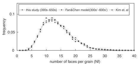
Next, we refer to the face distribution related results. The average face number shows the value of 14.0 at t¼ 32:5s[500t]. It decreases with simulation time and ap-proaches to a constant value of 13.7 at around t¼325 s[5000t]. The grain distribution with the number of faces per grain in Fig. 6, where the results from the phase-field simulation by Suwa et al. (Fan and Chen model+DGR), Kim et al. (MPF model, symbols were taken from Fig. 16 in Ref. 18)) and this study (MPF model+APT algorithm) are compared. Although the face number at which the distribu-tions have a maximum value is slightly different, they are almost identical. Finally, we consider the relationship between the average number of faces of per grain adjacent to an N-faced grain,mðNfÞ, and the face number in grains,Nf, at t¼390[6000t] (for 2¼6:0x-Case1). The linear relation similar to the Aboav-Weaire relations34,35)is calcu-lated between mðnÞandNf by the linear least-square fitting for simulation results as mðNfÞ Nf ¼13:6Nfþ27:2. The

relation is very close to those of mðNfÞ Nf ¼13:7Nfþ 24:7 andmðNfÞ Nf ¼13:3Nf þ23:4 obtained in Ref. 21) and Ref. 11), respectively.

4. Concluding Remarks

We performed computer simulations of normal grain growth in 3D by using the MPF model. For the purpose of the acceleration of computation, we applied both the APT algorithm and the parallel coding techniques to the MPF model. We have reconfirmed that the MPF is a powerful tool for simulating grain growth. Especially, the procedure described in this paper is highly efficient. As mentioned in Section 2.2, the implementation of the parallelization was quite easy. Further, the memory consumption of our procedure was 1/3 of that in Ref. 21) (Fan and Chen model with the DGR algorithm and the parallel coding techniques) even for the simulation of the normal grain growth. The difference will be larger with the introduction of anisotropy into grain boundary properties. As pointed out by Kim et al.,18) _{the easiness of the calculating topological} character-istics of grains is an advantage of MPF+APT scheme.

Aknowledgements

This study was partially supported by the Next Generation Supercomputer Project, Nanoscience Program, MEXT, Japan. It was also supported by the CREST, Japan Science and Technology Agency.

REFERENCES

1) H. V. Atkinson: Acta Metall.36(1988) 469–491.

2) D. Weaire and J. A. Glazier: Materials Science Forum94–96(1992) 27–38.

3) M. Hillert: Acta Metall.13(1965) 227–238.

4) J. E. Burke and D. Turnbull: Prog. Metal Phys.3(1952) 220–292. 5) N. P. Louat: Acta Metall.22(1974) 721–724.

6) D. Weaire and F. Bolton: Phys. Rev. Lett.65(1990) 3449–3451. 7) D. Weaire and J. P. Kermode: Phil. Mag.B48(1983) 245–249. 8) D. Weaire and H. Lei: Phil. Mag. Lett.62(1990) 427–430.

9) K. Kawasaki, T. Nagai and K. Nakashima: Phil. Mag.B 60(1989) 399-421.

10) C. V. Thompson, H. J. Frost and F. Spaepen: Acta Metall.35(1987) 887–890.

11) F. Wakai, N. Enomoto and H. Ogawa: Acta Mater.48(2000) 1297–

1311.

12) M. P. Anderson, D. J. Srolovitz, G. S. Grest and P. S. Sahni: Acta Metall.32(1984) 783–791.

13) D. J. Srolovitz, M. P. Anderson, P. S. Sahni and G. S. Grest: Acta Metall.32(1984) 793–802.

14) D. Fan and L.-Q. Chen: Acta Mater.45(1997) 611–632.

15) D. Fan, C. Geng and L.-Q. Chen: Acta Mater.45(1997) 1115–1126.

16) A. Kazaryan, Y. Wang, D. A. Dregia and B. R. Patten: Acta Mater.50 (2002) 2491–2502.

17) N. Ma, A. Kazaryan, D. A. Dregia and Y. Wang: Acta Mater.50(2002) 3869–3879.

18) S. G. Kim, D. I. Kim, W. T. Kim and Y. B. Park: Phys. Rev.E 74

(2006) 061605-1–061605-14.

19) J. A. Warren, R. Kobayashi, A. Lobkovsky and W. C. Carter: Acta Mater.51(2003) 6035–6058.

20) C. E. Krill and L.-Q. Chen: Acta Mater.50(2002) 3057–3073. 21) Y. Suwa, Y. Saito and H. Onodera: Comput. Mater. Sci.40(2007) 40–

50.

22) Y. Suwa, Y. Saito and H. Onodera: Scripta Mater.55(2006) 407–410.

0 0.05 0.1

0

number of faces per grain (Nf)

frequency

this study (390s−650s) Fan&Chen model(300s’−600s’) Kim et. al

40 35 30 25 20 15 10 5

Fig. 6 Distributions of grains with the number of faces per grain in the 3D simulations; Suwaet al.21)_{(Fan and Chen model+DGR), Kimet al.}18)

[image:5.595.52.285.68.177.2]

23) S. Vedantam and B. S. V. Patnaik: Phys. Rev.E 73(2006) 016703-1– 016703-8.

24) J. Gruber, N. Ma, Y. Wang, A. D. Rollett and G. S. Rohrer: Model. Simul. Mater. Sci. Eng.14(2006) 1189–1195.

25) I. Steinbach and F. Pezzolla: PhysicaD 134(1999) 385–393.

26) F. J. Humphreys and M. Hatherly: Recrystallization and related

annealing phenomena, (Pergamon, Oxford. 1995).

27) S. G. Kim, W. T. Kim, T. Suzuki and M. Ode: J. Crystal Growth261 (2004) 135–158.

28) Y. Suwa, Y. Saito and H. Onodera: Acta Mater55(2007) 6881–6894. 29) S. Sakamoto and F. Yonezawa: Kotai Butsuri (Solid State Physics),24

(1989) 219–226.

30) A. A. B. Sugden and H. K. D. H. Bhadeshia:Recent Trends in Welding Science and Technology, ed. by S. A. David and J. M. Vitek, (ASM International, Ohio, USA, 1989) pp. 273–278.

31) D. Weaire and S. Hutzler: The Physics of Foams. Oxford, Clarendon press. 1999.

32) D. Zo¨llner and P. Streitenberger: Scripta Mater.54(2006) 1697–1702. 33) P. Streitenberger and D. Zo¨llner: Scripta Mater.55(2006) 461–464.

34) D. A. Aboav: Metallography,5(1970) 251–263.