Bayesian Analysis of Type I Censored Data from Two-Parameter Exponential Distribution

Abstract—The parameters of the two parameter exponential distribution are estimated in this article based on complete and Type-I censored samples from the Bayesian viewpoint. Bayes point estimates and credible intervals for the scale and location parameters are derived under the assumption of squared error loss function. An illustrative example is provided to motivate the proposed Bayes point estimates and the credible intervals. The proposed Bayes estimates and the maximum likelihood estimates are compared via Monte Carlo simulations.

Index Terms— Bayes estimate, Censored samples, Credible interval, Exponential distribution.

I. INTRODUCTION

ET X1,X2,...,Xn be a random sample of size n from a

two parameter exponential distribution with scale parameter  and location parameter , denoted byE(,), where  and  are independent. The probability density function (p.d.f) of X at x is:

) (

) , |

(x   e x

f ;0x and 0 (1) This distribution plays an important role in survival and engineering reliability analysis; see for example Balakrishnan and Basu [2].

In life testing experiments, it often happens that the experiment is censored in the sense that the experimenter may not be in a position to observe the life times of all items put on test because of time limitations and other restrictions on the data collection. The two most common censoring schemes are Type-I and Type-II censoring schemes. In Type-I censoring scheme, the experiment continue up to a preselected fixed time T but the number of failures is random, whereas in Type-II censoring scheme, the experimental time is random but the number of failures is fixed, k.

Manuscript received Feb 28, 2012; revised Mar 31, 2012.

This work was financially supported by Fahad Bin Sultan University, Tabuk, Saudi Arabia.

Husam Awni Bayoud, Arts and Sciences Unit, Fahad Bin Sultan University, Tabuk, Saudi Arabia, P.O. Box 15700 Tabuk 71454. Phone: 00966 5 66014964; fax: 00966 4 42 76 919; e-mail: [email protected].

The estimation of these parameters based on Types I and II censored samples has been considered by several authors in the literature from the Bayesian point of view. El-Sayyed [5] has derived Bayes estimate and unbiased estimate for

1





. Singh and Prasad [6], [3] have considered the problem of estimating the scale parameter



1. They propose some empirical Bayes estimators for



1 under the situation that the scale parameter



is known. Ye and Yang [4] considered the empirical Bayes estimation of location parameter of two parameter exponential distribution under Type-II censoring model. Sarhan [1] studied empirical Bayes estimates in one parameter exponential distribution, Zhou [10, 11] considered Bayes estimation and prediction for one and two parameter exponential distribution. Singh and Kumar [7, 8] proposed Bayes estimators for exponential scale parameter under multiply type II censoring. Singh and Kumar [9] proposed Bayes point estimates for the scale parameter under type-II censoring by using generalized non-informative prior and natural conjugate prior. Shi and Yan [12] proposed empirical Bayes estimate for the scale-parameter under Type-I censored sample assuming known location parameter.

It is noted that in many practical applications, the value of the parameter



may not be known.Therefore, it is useful and important to consider the problem of estimation for the parameter



when



is unknown.

This paper aims to derive Bayes point estimates and credible intervals for the scale and location parameters of a two exponential distribution based on complete and Type-I censored samples separately. Bayes point estimates are proposed under the assumption of the squared error loss function.

The scale parameter



is assumed to follow exponential distribution with hyper parameterA, and the location parameter  is assumed to follow uniform distribution from zero to B. Suggestions for choosing the hyper parameters

A _and B are provided.

The rest of this paper is organized as follows: Section 2 describes the probability models that are needed in this work. Bayes point estimates for the scale and location parameters are proposed in Section 3 based on complete and Type-I censored samples separately. Credible intervals for those parameters are derived in Section 4. An illustrative example is provided in Section 5. Finally, the main conclusions are included in Section 6.

Bayesian Analysis of Type I Censored Data

from Two-Parameter Exponential Distribution

Husam Awni Bayoud, Member, IAENG

II.MODELS A. Complete Sample

Let X1,X2,...,Xn ~E(,), the p.d.f of X is given in (1.1). The likelihood function of the complete sample

n X X

X₁, ₂,..., given  and  is given by:





       n i i x n n e x x x

L _{, ,..., | ,} 1

2 1    

 (2) The parameter  is assumed to follow an exponential distribution with p.d.f given by:

g()AeA; A0 (3) where the hyper parameter A is a preselected positive real number that is chosen to reflect our beliefs about the expected value of



1

, because the expected value of



equals

A 1

.

The parameter  is assumed to follow a uniform distribution with p.d.f given by:

B B

p() 1; 0 (4) where the hyper parameter B is a preselected nonnegative real number that is chosen to reflect our beliefs about the lower bound of the x's , which can be easily assumed to equal the minimum observed value, x(1).

In order to construct the Bayes estimates for  and , the joint posterior p.d.f of  and  given the observations



x₁,x₂,...,xn



is derived in this section for the complete sample



x₁,x₂,...,xn



.

The joint posterior p.d.f of  and  given



x₁,x₂,...,xn



is given by:







    



    

  _B n n n C d d p g x x x L p g x x x L x x x h 0 0 2 1 2 1 2 1 , | ,..., , , | ,..., , ,..., , | ,               ) ( ] [ 1 n C e n n i i x A n           (5)

where _{n n}

E D

C 1  1 in which   







 n i i B x A D 1 and     n

i xi

A E

1

, 0 and 0B.

The marginal posterior p.d.f of



given



x₁,x₂,...,xn



is given by:







 



      E D n B n n C e e n C d x x x h x x x h       _ ) ( ,..., , | , ) ,..., , | ( 1 0 2 1 2 1 , (6)

where 0, D,E and Care defined in (5).

The marginal posterior p.d.f of



given



x₁,x₂,...,xn



is given by:









1

1 2 0 2 1 2 1 , 1 ,..., , | , ) ,..., , | (              _ n n i i n n C x A C n d x x x h x x x h       (7)

where 0Bx(1) and Cis defined in (5).

B. Type I Censored Sample

In type-I censored samples, suppose that a random sample of n units is tested until a predetermined time T (x(1)) at

which time the test is terminated. Failure times for k observations are observed, where k is a random variable. Thus the lifetimes are observed only ifxi T; i1,2,...,n.

Let       T x T x i i i ; 1 ; 0 

Therefore, 

  n

i i

k

1

 , which is assumed to be greater than zero. The likelihood function in this case is given by:



_{x x x T}



_{f x} i _{F T} i

L n

i i

n

I        

 

 1

1 2

1, ,..., | , , [ ( | , )] [1 ( | , )]

 









 

k_e x _e Tn k n n

i i i   





 1 ₍₈₎

The joint posterior p.d.f of  and  based on the type-I censored sample is given by:







    



    

, | ,..., , , | ,..., , , ,..., , | , 0 0 2 1 2 1 2 1    B n I n I n I d d p g x x x L p g x x x L T x x x h            

where g() and p() are defined in (3) and (4) respectively. Therefore





  ) ( , ,..., , | , 1 2 1 1 k C e n T x x x h A n k n T x n I n

i i i

                  

 (9)

where 0, 0B and 1 1 0 1 1

1 _k  _k 

E D

C in which



n k



nB T

A x

D n

i i i

      1

1  and E x A T



n k



n

i i i

     1

1  .

The marginal posterior p.d.f of



given



x₁,x₂,...,x_n;T



is given by:





      _                1 1 ) ( , ,..., , | , ) , ,..., , | ( 1 1 0 2 1 2 1 , E D k B n I n I e e k C d T x x x h T x x x h (10)

The marginal posterior p.d.f of given



x1,x2,...,xn,T



is given by:





   0 2 1 2 1 , (| , ,..., , ) ,| , ,..., , 

 x x x T h x x x T d

h I n I n





1

1 1 1 _             _k n

i xi i T n k n A

C k n   (11)

where 0Bx(1) and C1is defined in (9).

III. POINT ESTIMATION of  and  In this section, Classical and Bayesian estimation for  and  are proposed using the complete and Type-1 censored samples separately. The squared error loss is assumed to construct the Bayes estimates.

A. Estimation from Complete Sample

In the case of complete sample, the Bayes point estimate

C



ˆ _of

_

_{under the squared error loss is the mean of the} marginal posterior p.d.f of



given in (6), which is given by:     0 2 1 , , ( ) ( | , ,..., )

ˆ _{   }

_C E_{h C} h_C x x x_n d

_        _{ } 1 1 1 1 n n _E D C n (12) The Bayes point estimate



ˆ of



under the squared error loss is the mean of the marginal posterior p.d.f of



given in (7), which is given by:





 _h B _{C n}

C E _C h x x x d

0 2 1 , ( | , ,..., ) ) ( ˆ ,      _  _                 _{ } 1 1 1 1 ) 1 ( 1 1

_{n n n}

E D n n D B C (13)

The MLE of



and



from the complete sample are respectively:     _n i i C MLE x x n 1 ) 1 ( , ) ( ˆ

 and ˆMLE,C x(1)

B. Estimation from Type I Censored Sample

In the case of type-I censored sample, the Bayes point estimate



ˆ_I of



under the squared error loss is the mean of the marginal posterior p.d.f of



given in (10), which is given by:     0 2 1 , ( | , ,..., ) ) ( ˆ ,    

_I E_{h I} h_{ I} x x x_n d

          _{ } 1 1 1 1 1 1 1 _{k k} E D C k (14)

The Bayes point estimate



ˆI of



under the squared error

loss is the mean of the marginal posterior p.d.f of



given in (11), which is given by:





 _h B _{I n}

I E _I h x x x d

0 2 1 , ( | , ,..., ) ) ( ˆ ,      _{ }                     _{ } 1 1 1 1 1 1 1 1 ) 1 ( 1 1 k k

k _{n k D E}

D B

C (15)

The MLE of



and



from the type-I censored sample are respectively: ) 1 ( 1 , ) ( ˆ x n k n T x k n

i i i

I MLE       

 and ˆMLE,I x(1)

IV. CREDIBLE INTERVALS for  and  A. Based on Complete Sample

Based on the complete sample x1,x2,...,xnand by using the

posterior density function of  that is defined in (6), the equal- tailed



1



100% credible interval for  is



L,U



that satisfies: 2 )] 0 , ( ) , ( [ 1 )] , ( ) 0 , ( [ 1 ) ( 1                                  n E n E D n n D n C L n L n and 2 ) , ( 1 ) , ( 1 1 1 1 1 ) ( ) ( 1                                                                                        U n U n n U n U U n n E n E D n D E E E D n n C

where



     z t a _{e dt} t z

a 1

) ,

( , the incomplete gamma function. Similarly, by using the posterior density function of



that is defined in (7) the equal-tailed



1





100% credible interval for



is





L,



U



; where

n A x x A C n i i n n n i i L                                  1 1 1 1 2 





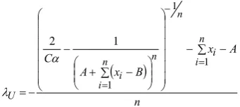
n A x B x A C n i i n n n i i U                                   1 1 1 1 2  

B. Based on Type-I Censored Sample

Based on a Type-I censored sample and by using the posterior density function defined in (10), the equal- tailed



1





100% credible interval for  is



L,I,U,I



that

satisfies: 2 )] 0 , ( ) , ( [ 1 )] , ( ) 0 , ( [ 1 ) ( 1 , 1 1 , 1 1 1                                  k E k E D k k D k C I L k I L k , and 2 )} , ( 1 ) , ( 1 1 1 1 1 { ) ( 1 , 1 1 , 1 1 , 1 , 1 , 1 1 1                                                                             I U k I U k k I U k I U I U k k E k E D k D E E E D Γ(k) k C

Similarly, by using the posterior density function of



that is defined in (11) the equal- tailed



1





100% credible interval for



is





_L,_I,



_U,_I



; where









n k n T x A A k n T x C n

i i i

k

k n

i i i

I L                                      1 1 1 1 , 1 2     and

 

 

n k n T x A A B n k n T x C n

i i i k

k n

i i i

I U                                       1 1 1 1 , 1 2 _   

V. NUMERICAL EXAMPLE

Using Mathematica 5, if U has a Uniform(0,1) distribution, then x that satisfies U 1e(x) follows E(



,



). Let

[image:4.595.52.223.52.128.2]

Data I = {1.2373, 1.25419, 1.54525, 1.38357, 1.2655} be a random sample of size 5 generated from E(4,1).

Table 1 summarizes the values of ML and the Bayes estimates for the scale and location parameters obtained from data I. Those estimates were computed based on the complete and Type-I censored samples. The hyper parameters A and B were assumed to equal one over of the available sample's mean and the minimum observation respectively.

Based on the complete sample, the MLE of the parameters



and



are respectively:

0137 . 10 ) ( ˆ 1 ) 1 ( ,      n i i C MLE x x n

 and

2373 . 1 ˆ ) 1 (

,Cx 

MLE



The proposed Bayes estimates are         _{ } 1 1 1 1 ˆ n n C E D C n

 , and

1 1 ) 1 ( 1 1 ˆ 1

1 _

             

 _{n n n}

C E D n n D B C  .

The hyper parameters A and B are assumed to equal

747854 0 6858 6 5 1 .   



 . x n A n i i

andBx₍₁₎1.2373.

So,C0.331371, D1.24717 and E7.43365. Therefore

00952 . 4 ˆ

,C  B

 , and ˆ_B,C1.17514.

Based on Type-I censored sample, two schemes are studied, when T1.3 and T 1.5.

When T1.3, the MLEs are ˆ_MLE,I 17.5957 and

2373 . 1 ˆ ) 1 (

,I x 

MLE

 . The hyper parameters A and B are

assumed to equal 0.798514

1     n

i i i

x k A  and 2373 . 1 ) 1 (  x

B . So, C₁1.09631, D₁0.96901 and

15549 . 7

1

E .Therefore ˆ_B,I 3.10261,and ˆ_B,C1.14502. When T 1.5, the MLEs are ˆ_MLE,I 8.80927 and

2373 . 1 ˆ ) 1 (

,I x 

MLE

 . The hyper parameters A and B are

assumed to equal 0.778127

1     n

i i i

x k A  and 2373 . 1 ) 1 (  x

B . So, C₁0.433463, D₁1.23219 and

41868 . 7

1

E . Therefore ˆ_B,I 3.2483, and ˆ_B,C 1.15641. It becomes apparent from this study that the Bayes estimates give excellent results and it performs, in terms of the mean square error MSE, better than the MLE for estimation the parameters



and



based on both complete and Type-I censored schemes.

The 95% credible interval for the parameters



and



are summarized in Table 1 based on the complete sample and Type-I censored samples with T 1.3 and

5 . 1



[image:5.595.299.555.76.288.2]

TABLE I

95% CREDIBLE INTERVALS for  and  for the EXAMPLE

Param eter

based on Complete sample

based on Type-I censored sample with

3 1. 

T

based on Type-I censored sample with T1.5

 (0.97, 1.41) (1.25, 1.37) (1.24, 1.42)

 (1.30, 8.21) (0.66, 7.46) (0.89, 7.12)

Table 1 shows that the proposed credible interval gives reasonable estimates for



in all cases. It can be observed from this table that this credible interval estimates



by reasonable values only when the complete sample is used, and it gives bad lower bound when Type-I censored schemes are used.

VI. SIMULATION STUDIES

In this section, the performance of the MLE and the proposed Bayes estimates of



and



is investigated through a simulation study based on both complete and various Type-I censored schemes. The simulation study is carried out for various values of the combination





,



,n,T



; for (,)(0.5,2), (3,0.3), (1,1)

[image:5.595.41.295.543.764.2]

and (2,0), the termination time T is assumed arbitrary to equal 8 and 10. The hyper parameters A and B are assumed to equal one over the available sample mean and the minimum observed value, x(1) respectively. 1000 simulated datasets are generated from E(



,



) by using Mathematica 5. For the purpose of comparison, the average value of the MLE and the proposed Bayes estimates along with the mean squared error (MSE) in parentheses are reported by assuming n5 and 10 in Table 1 and Table 2 respectively. Estimators with the smallest MSE values are preferred.

TABLE II

EXPECTED MLE and BE along with MSE when n5

Parameter

Based on Complete Sample

(n5)

Based on Type-I Censored Sample

(T8)

Based on Type-I Censored Sample

(T10) MLE BE MLE BE MLE BE

5 0.



 0.85 (0.41)

0.80 (0.28)

0.85 (0.41)

0.80 (0.28)

0.85 (0.41)

0.79 (0.29)

2



 2.43

(0.39) 2.08 (0.22)

2.43 (0.39)

2.08 (0.22)

2.04 (0.33)

2.05 (0.18)

3



 5.2

(18.4) 1.77 (1.55)

5.2 (18.44)

1.77 (1.55)

5.04 (13.61)

1.77 (1.55)

3 0.



 0.37 (0.01)

0.26 (0.01)

0.37 (0.01)

0.26 (0.01)

0.37 (0.01)

0.27 (0.01)

1



 1.66 (1.34)

1.33 (0.40)

1.66 (1.34)

1.33 (0.40)

1.66 (1.73)

1.32 (0.43)

1



 1.18 (0.07)

0.99 (0.03)

1.18 (0.07)

0.99 (0.03)

1.20 (0.08)

1.01 (0.04)

2



 3.37 (9.73)

1.31 (0.51)

3.38 (9.73)

1.31 (0.51)

3.33 (7.2)

1.30 (0.53)

0



 0.1

(0.02) 0.06 (0.01)

0.095 (0.18)

0.058 (0.01)

0.097 (0.02)

0.058 (0.01)

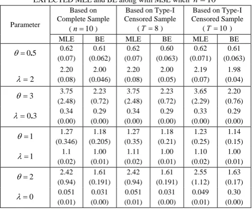
TABLE III

EXPECTED MLE and BE along with MSE when n10

Parameter

Based on Complete Sample

(n10)

Based on Type-I Censored Sample

(T8)

Based on Type-I Censored Sample

(T10) MLE BE MLE BE MLE BE

5 0.



 0.62 (0.07)

0.61 (0.062)

0.62 (0.07)

0.60 (0.063)

0.62 (0.071)

0.61 (0.063)

2



 (0.08) 2.20 2.00 (0.046)

2.20 (0.08)

2.00 (0.05)

2.19 (0.07)

1.98 (0.04)

3



 3.75 (2.48)

2.23 (0.72)

3.75 (2.48)

2.23 (0.72)

3.65 (2.29)

2.20 (0.76)

3 0.



 0.34 (0.00)

0.29 (0.00)

0.34 (0.00)

0.29 (0.00)

0.33 (0.00)

0.29 (0.00)

1



 1.27 (0.346)

1.18 (0.205)

1.27 (0.35)

1.18 (0.21)

1.23 (0.25)

1.14 (0.15)

1



 1.1

(0.02) 1.00 (0.01)

1.11 (0.02)

1.00 (0.01)

1.10 (0.02)

1.00 (0.01)

2



 2.42 (0.94)

1.61 (0.191)

2.42 (0.94)

1.61 (0.191)

2.55 (1.12)

1.63 (0.17)

0



 0.051 (0.01)

0.031 (0.00)

0.051 (0.01)

0.031 (0.00)

0.049 (0.01)

0.30 (0.00)

In terms of the MSE, It becomes apparent from Tables 2 and 3 that the proposed Bayes estimates perform better than the MLE based on complete and Type-I censored samples. It can be also noticed from those tables that the MLE and the proposed Bayes estimates perform better as n increases.

VII. CONCLUSIONS

In this article, a procedure for estimating the scale and location parameters,  and , of a two parameter exponential distribution was developed based on complete and Type-I censored samples. This approach was adopted from Bayes point of view. Prior probability distributions for the parameters  and  were assumed to be exponential and uniform distributions respectively. Bayes point estimates and credible intervals for  and  were proposed in the cases of complete and Type-I censored samples under the squared error loss. It was shown from simulation studies that the proposed Bayes estimate performed better than the MLE for estimation  in the case of Type-I censored sample. Moreover, the proposed credible interval gave excellent results for estimation the parameters  and  based on complete samples.

REFERENCES

[1] A.M. Sarhan, “Empirical Bayes estimates in exponential reliability model,” Applied Mathematics and Computation, vol. 135, pp. 319-332, 2003.

[2] Balakrishnan, “On the Maximum likelihood Estimation of the location and scale parameters Exponential Distribution Based on Multiply Type II censored Samples,” Journal of Applied Statistics, vol. 17, pp. 55-61, 1990.

[3] B. Prasad and R. S. Singh, “Estimation of prior distribution and empirical Bayes estimation in a non-exponential family,” J. Statist. Plann. Inference, vol. 24, pp. 81-86, 1990.

[4] E.H. Ye and J.L. Yang, “EB estimation of location-parameter of two-Parameter meter exponential lifetime distribution for the Type-II Censoring model,” Journal of Nanjing University of Aeronautics &

Astronautics, vol. 3, pp. 333-340, 1995.

[5] G. M. El-Sayyed, “Estimation of the parameter of an exponential distribution,” Journal of Royal Statistical Society: Series B (Statistical

[6] R. S. Singh and B. Prasad, “Uniformly strongly consistent prior distribution and empirical Bayes estimators with asymptotic optimality and rates in a non-exponential family,” Sankhya A, vol. 51, pp. 334-342, 1989.

[7] U. Singh and A. Kumar, “Shrinkage estimators for exponential scale parameter under multiply type II censoring,” Austrian Journal of Statistics , vol. 34, pp. 39-49, 2005a.

[8] U. Singh and A. Kumar, “Bayes estimator for one parameter exponential distribution under multiply-II censoring,” Indian Journal

of Mathematics and Mathematical Sciences, vol. 1, pp. 23-33, 2005b. [9] U. Singh and A. Kumar, “Bayesian Estimation of the Exponential

Parameter under a Multiply Type-II Censoring Scheme,” Austrian Journal of Statistics, vol. 36, no. 3, pp. 227-238, 2007.

[10] Y.Q. Zhou, “Prediction problem for exponential distribution,”

Structure and Environment Engineering, vol. 2, pp. 1-13, 1998. [11] Y.Q. Zhou , W.S. Liu and S.L. Tian, “Reliability assessment of

two-parameter exponential distribution,” Quality & Reliability, vol. 1, pp. 5-10, 2004.