Performance Prediction Model for Distributed
Applications on Multicore Clusters
Nontokozo P. Khanyile, Jules-Raymond Tapamo, and Erick Dube
Abstract—Distributed processing offers a way of successfully dealing with computationally demanding applications such as scientific problems. Over the years, researchers have investi-gated ways to predict the performance of parallel algorithms. Amdahl’s law states that the speedup of any parallel program has an upper bound which is determined by the amount of time spent on the sequential fraction of the program, no matter how small and regardless of the number of processing nodes used. This research discusses some of the short comings of this law in the current age. We propose a theoretical model for predicting the behavior of a distributed algorithm given the network restrictions of the cluster used. The paper focuses on the impact of latency and bandwidth which affect the cost of interprocessor communication and the number of processing nodes used to predict the performance. The model shows good accuracy in comparison to Amdahl’s law.
Index Terms—Latency, propagation delay, distributed pro-gramming, bandwidth, performance.
I. INTRODUCTION
D
ISTRIBUTED systems are collections of autonomous computing systems which are connected by some net-work and net-work together to solve an overall task using the notion of divide and conquer. The total processing time of a distributed program is calculated as the total communi-cation time plus the total computation time. It is always unnerving to know what to expect from a system before it is actually developed. Clients often need to know the expected performance so that they can make an informed decision on whether or not to invest in a project. Amdahl came up with a law for predicting performance of parallel systems. However, there has been much criticism surrounding Amdahl’s law for its assertion that parallel processing is unscalable. Amdahl’s law stipulates that even when the serial fraction of a problem, say s, is considerably small, the maximum speedup obtain-able is only 1s even with an infinite number of processing nodes [1]. Ifs is the time spent byN processors executing the serial fraction of the computation time of a program and pis the time spent executing the parallel portion, then Amdahl’s law states that the estimated speedup is given by:Speedup= 1
(s+Np), with s=1-p (1) Manuscript received March 17, 2012; revised April 10, 2012. This work was supported in part by the South African Council for Scientific and Industrial Research (CSIR).
N.P. Khanyile is with the Modelling and Digital Sciences (Information Security) Division of the Council for Scientific and Industrial Research, Pretoria, South Africa and the School of Electrical, Electronic and Computer Engineering, University of KwaZulu-Natal, Durban, South Africa (e-mail: [email protected]).
J.-R. Tapamo is with the School of Electrical, Electronic and Computer Engineering, University of KwaZulu-Natal, Durban, South Africa.
[image:1.595.311.539.163.276.2]E. Dube is with the Modelling and Digital Sciences (Information Security) Division of the Council for Scientific and Industrial Research, Pretoria, South Africa.
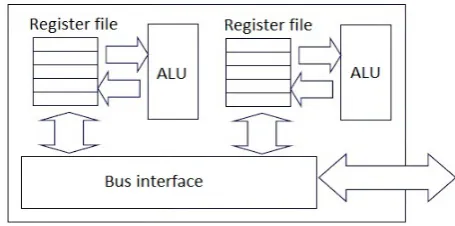
Fig. 1. Structure of a dual-core system
Amdahl’s law assumes that the problem size remains fixed after parallelization. This, however, is not always the case. It has been shown that in practise, parallel processing workload often scales up with the number of processing nodes (except for academic research purposes) [1], [2]. Gustafson [1] discussed the concept of scalable parallel processing and introduced the scaled-sized model for speedup, which was later revised into fixed-time model by Sun & Chen [2] for multicore hardware systems. Gustafson [1], Hill & Marty [3] and Sun & Chen [2] argue that workload of parallel problems should scale up with the increasing computing capability in powerful machines as these machines are designed for large problems. According to Gustafson, parallel workload of massively parallel systems varies linearly with the number of processors, and hence the scaled-sized speedup model is a linear function of the number of processors. Although Hill & Marty successfully model the performance of parallel processing on multicore systems, they do not cater for distributed multicore systems.
Distributed computation differs from parallel computation in the way in which memory is used. In parallel systems, all processing elements use the same shared memory for communication, whereas distributed systems are autonomous systems with private memory connected by a network which is used for communication between the processing nodes. Fig. 1 shows an internal structure of a parallel/shared mem-ory system in the form of a dual-core system, while Fig. 2 shows an example of a multicore distributed system, where multicore machines are combined by a network to function as one.
Fig. 2. Example structure of a multicore cluster
a way of predicting performance for code distributed on multicore clusters. The rest of the paper is organised in the following manner: Section 2 discusses the factors which influence the performance of a distributed system. Section 3 gives the related works and background. Section 4 discusses the proposed performance model. Section 5 analyzes the results and Section 6 concludes the paper.
II. FACTORSAFFECTINGPERFORMANCE IN
DISTRIBUTEDSYSTEMS
The performance of a distributed algorithm is affected by more than just the application efficiency and the number of processing nodes used. Since clusters are connected by networks, network factors like latency and bandwidth have a considerable impact on the performance of a distributed system. As such, it is necessary to take into account the network influence when predicting the performance of these systems.
Bandwidth and latency capture the volume and time di-mensions of information processing, respectively. Latency measures the time taken to complete a request, while band-width measures the volume of information transmitted in a time interval [4]. The next subsections go into greater detail about the factors that impact information processing performance.
A. Application Efficiency
If an algorithm is not efficient in its execution, even the most powerful machines can not improve its performance. There are a lot of ways to help improve the efficiency of parallel programs. Code has to be optimized on two levels; per-processors and across processors, (i.e. each core of a multicore machine and communication across the clus-ter). Optimization techniques include code modifications and compiler optimizations. Per-processor optimizations include but no limited to, loop optimization, floating point arithmetic optimization, prefetching, and use of optimized mathematical libraries. Across processors optimizations mainly deal with minimizing communication, reducing overhead associated with communication through the use of efficient network in-terconnections. Using latency hiding techniques to reduce the effects of latency. These techniques include using operations such as MPI Isend/IRecv [5] which enable an application to send data before it is needed and keep working while sending. Compilers like GNU come with optimization flags such as-ffast-mathwhich optimizes mathematical functions.
B. Application Latency
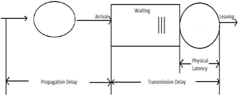
Application latency is defined by Shaffer [6] as the total amount of time that an application has to wait for a response after issuing a request for some data. The application delay reflects the total wait time incurred by the system, including all subsystems and kernel overhead as well as network latency [6]. Network latency is the time spent waiting, from the instantiation of an operation until the return of the desired results [6]. A distinction can be made amongst the different types/sources of network latency. Three types of network latencies are discussed; the propagation delay, transmission delay, and physical latency. Fig. 3 is a representation of these two network latency sources as a single server open queueing system.
Fig. 3. Network latency presented as a propagation and transmission delay server (adapted from [4])
1) Propagation Delay: Propagation delay is defined as the time taken waiting for the last bit to arrive plus the overhead that comes with the device [6]. The propagation delay can not be eliminated or avoided because the speed of light is inviolable [6]. Transmission speed can not be improved beyond propagation delay. A propagation of a certain system indicates the maximum transmission rate that the system can achieve.
2) Physical latency: Physical latency measures the pro-cessing time on a device without waiting (i.e. the service time). It varies according to device utilization or load [4]. The physical latency can be halved to double the bandwidth. Ding [4] showed that halving the physical latency yields better results than actually doubling the bandwidth. The system is able to perform twice the amount of work without saturation. 3) Transmission Delay: Transmission delay is the amount of time taken to transmit all the packet’s bits into the link. In most networks, transmission of packets occurs in a first come first serve manner, which results in queueing for transmission rates that are not high [7]. It is determined by the packet size and the transmission rate of the network and not at all affected by the distance.
C. Bandwidth
[image:2.595.307.547.238.336.2]does not automatically guarantee performance gain. In order to benefit from high bandwidth, software often needs to be modified in order to leverage the high bandwidth. For example, applications developed for 32-bit systems may run slower on 64-bit systems [4].
III. RELATEDWORK
Performance prediction methods in literature can be clas-sified into three categories; analytical [1], [2], [6], [8]– [10], profile-based [11], [12] and simulation-based [13]–[16]. This paper uses an analytical approach based on Sun & Chen’s [2] and Shaffer’s [6] works. Analytical solutions have the advantage of efficiency over the rest of the prediction methods, however, it is limited by the fact that many complex systems are analytically intractable [17]. While Amdahl’s law is only concerned with software, Hill & Marty’s corollary is hardware-based. Sun & Chen’s study which revises Hill & Marty’s work assumes a symmetric architecture with each core having its own L1 cache, where the memory bound is the cumulated capacity of the L1 caches. Following the conclusion made by Hill & Marty that the symmetric multicore architecture has a speedup of:
Speedup= 1−f 1
perf(r)+
f.r perf(r).n
(2)
whereperf(r)is defined as the sequential performance of a powerful core withrBase Core Equivalents (BCEs). Sun & Chen’s fixed-time speedup model for multicore architectures reveals the scalability of multicore architectures. Sun & Chen define the fixed-time speedup as:
SpeedupF T =
Sequential Time of Solving Scaled workload Parallel Time of Solving Scaled workload
(3) Let w be the original workload and w0 be the scaled workload. Supposing the time taken to processwsequentially is the same as the time taken to processw0 in parallel using
m processors. Assuming that the scale of the workload is only on the parallel portion;w0 becomes:
w0= (1−f)w+mf w (4)
Therefore
SpeedupF T =
Sequential Time of Solving w’ Parallel Time of Solving w’ (5)
SpeedupF T =
Sequential Time of Solving w’ Sequential Time of Solving w (6)
w0 w =
(1−f)w+mf w
w = (1−f) +mf (7)
which gives Gustafson’s law [1]. The scaled-sized model assumes that the scaling is only at the parallel portion. Based on this assumption and following (2), Sun & Chen constructed the fixed-time speedup model to be:
(1−f)w perf(r) +
f w perf(r) =
(1−f)w perf(r) +
f w0
perf(r)m (8)
If we let n = mr be the scaled number of cores, with
n = r being the initial point, then w0 = mw. The final scaled speedup compared withn=r becomes:
SpeedupF T =
Sequential Time of Solving w’ Sequential Time of Solving w
=
(1−f)w perf(r)+
f w0 perf(r)
w perf(r)
= (1−f) +mf
(9)
The fixed-time speedup model demonstrates the scalability of multicore systems. Like the scaled-sized model, it is linearly dependent on the number of processors m. Efficiency of a parallel algorithm is measured by the speedup attained. If
T1 is the execution time for the serial implementation, the speedup can be computed as T1
TN, whereTN is the execution
time attained when using N processors. Efficiency is then calculated as:
EN =
TN
N (10)
An efficient algorithm attains a speedup close to N for every TN, (i.e. EN = 1). It has been established in the
literature that for distributed systems, this is not always the case. As the number of processors increases, speedup of the distributed systems starts to decline. This is usually because of the increased interprocessor communication, known as message passing. Adding computation nodes increases the networks communication links which ultimately increases propagation delay.
IV. PERFORMANCEMODEL
This research focuses on the performance of multicore clusters. Multicore clusters are ideal for hybrid programming, (i.e. a mixture of distributed and parallel processing). While distributed programming deals with coarse grain parallelisa-tion, parallel programming focuses on fine grain parallelism within the computing nodes. It is clear to see the advantage in this form of an architecture. MPI can be used for the coarse grain parallelism and use p-threads or OpenMP for fine grain parallelism per node. While multicore systems are scalable and provide high performance, they have their limits. Writing thread-safe programs is not easy, especially as the number of threads increases. Enrico Clementi, a former IBM fellow and pioneer in computational techniques for quantum chemistry and Molecular dynamics, once said”I know how to make 4 horses pull a cart - I don’t know how to make 1024”. Introducing clustered systems relieves the strain of using too many threads on one machine.
A. Computational Cost
In distributed processing, an application can only run as fast as the slowest processor. Thus, following Sun & Chen’s fixed-time model, we redefineperf(r)to be:
perf(r0) =max(perf(ri)) (11)
whereperf(ri)is the sequential performance of a
power-ful core of a processing nodeiwithrBCEs. Using (9) and the assertion thatw0 =mw we get the following,
(1−f)w perf(r0)+
f w0 pref(r0)m =
(1−f)w perf(r0)+
f w perf(r0)
w perf(r0)
= (1−f)+mf
B. Communication Cost
The communication overhead associated with message passing can be quite large. Shaffer [6] proposed a theoretical predictive measure of communication cost in wide area distributed systems to be:
Comm T ime=m×[s
b +d×7.67×10
−6+] (13)
wheremis the frequency of messages needed during the task, b is the bandwidth in bits/second, is the overhead incurred per message and s andd represent the size of the message and the length of the communication channel in mile, respectively.
Propagation delay is normally calculated as the reciprocal of the speed of light which is currently 299792.458 km/s. However, Shaffer stated that this value is not the same for all types of cables. Different types of cables transmit at different speeds, which is less than the actual speed of light. This speed is known as the normal velocity of propagation (NVP). Optical fiber has an NVP close to 0.7 [6].
We define the cost of sending an L bit message between two processors as:
Tcomm(L)≤
L
τ + (σmax×dist) +L (14)
whereτ is the upper bound of the network latency,σmax
is the maximum delay incurred by the system, dist is the physical distance between the network points and (L) is the overhead associate each message of size L bits, i.e. the send and receive overhead.
V. EXPERIMENTS
The total estimated running time is calculated as:
TEST(m) =Tcomp(m) +Tcomm(m, L) (15)
where Tcomp(m) is the computation time as defined in
Section 4.1 and Tcomm(m, L) is the total time spent by m
nodes communicating messages of sizesL.
Tcomp(m) =Tseq/SpeedupF T (16)
Tcomm(m, L) =
X
Tcomm(L) (17)
Tseq is sequential time and SpeedupF T is defined in (12).
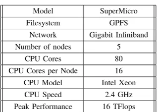
[image:4.595.90.250.658.771.2]The performance model was tested on two different applica-tions; one communication intensive and one computationally intensive. The experiments were performed on a cluster with the specifications given in table 1.
TABLE I SYSTEMCONFIGURATION
Model SuperMicro Filesystem GPFS
Network Gigabit Infiniband Number of nodes 5
CPU Cores 80
CPU Cores per Node 16 CPU Model Intel Xeon CPU Speed 2.4 GHz Peak Performance 16 TFlops
A. Application 1: Large Array Application
This application takes in two large array of numbers in two 1 MB files, then performs a series of mathematical functions (matrix multiplication, covariance matrix, trans-pose and eigenvectors) and finally writes back the results to a 4 GB file. The application has minimal interprocessor communication. Only the file names are broadcasted.
B. Application 2: Distributed Fingerprint Enhancement Ap-plication
The fingerprint enhancement application consists of a series of computationally intensive image processing oper-ations [18]. Image processing operoper-ations require intensive communication with neighbouring processors in order to access neighbouring pixels. Hence, the application has a lot of message passing making it a bit harder to scale with respect to processing nodes.
C. Results Analysis
The system used for testing has an NVP of 0.67, hence the expected propagation delay per km is
propagation delay= 1
299792.458∗0.67 = 0.0049ms
(18) Fig. 4 shows the prediction results vs. the observed per-formance of application 1. A comparison between Amdahl’s law and our model is made. Amdahl’s predictions show unscalability, performance does not improve beyond the 114 seconds mark. Our model shows great scalability and the error margins are better than those experienced by Amdahl’s law. Fig. 5 shows the results obtained through using the prediction model for application 2. From the graph, an increase in the communication time is evident as the number of processors increase. This is mainly due to the frequency of message passing during prefetching of boundary cells as well as the size of the messages. Fig. 6 plots the predicted per-formance of the fingerprint enhancement application against the observed performance using the model discussed in this paper, Amdahl’s law and Sun & Chen’s model. From Fig. 6 its clear to see that Sun & Chen’s model over estimates the speedup, whereas Amdahl’s law under estimates. Sun & Chen’s model does not consider the effects of communication associated with distributed systems. Amdahl’s law on the other hand performs better than Sun & Chen in this case. Our model does not give the exact estimates, it over estimates the speedup but the error margins are better than those experienced by Amdahl’s law and Sun & Chen’s model.
Application one has minimum communication (only two broadcast messages to share the filenames). In comparison to computation, communication time is insignificant hence the model becomes almost identical to that of Sun & and Chen’s.
VI. CONCLUSIONS
Fig. 4. Results of the predicted performance for the big array application. (a) Performance of the application using only one node. (b) Performance using two nodes. (c) Performance using three nodes. (d) Performance using four nodes. (e) Performance using five nodes
Fig. 5. Results of the predicted performance for the fingerprint enhance-ment application
ACKNOWLEDGMENT
We would like to thank the Center for High Performance Computing (CHPC) for granting us access to their clusters.
REFERENCES
[1] J. Gustafson, “Reevaluating amdahl’s law,” Communications of the ACM, vol. 31, pp. 532–533, May 1988.
[2] X.-H. Sun and Y. Chen, “Reevaluating amdahl’s law in the multicore era,”Journal of Parallel and Distributed Computing, vol. 70, pp. 183– 188, 2010.
Fig. 6. Predicted results vs observed results for fingerprint enhancement application
[3] M. Hill and M. Marty, “Amdahl’s law in the multicore era,”IEEE Computer, vol. 41, no. 7, pp. 33–38, 2008.
[4] Y. Ding, “Bandwidht and latency: Their changing impact on perfor-mance,” in Proc. 35th Computer Measurement Group Conference, 2005, pp. 67–78.
[5] M. P. I. Forum,MPI-2.2: A Message Passing Interface Standard, Sep 2009. [Online]. Available: http://www.mpi-forum.org.docs/docs.html [6] J. H. Shaffer, “The effects of high bandwidth networks on wide area
[image:5.595.57.287.468.612.2][7] J. Kurose and K. Ross,Computer Networks: A Top-Down Approach Featuring the Internet. Addison-Wesley, 2001.
[8] A. van Gemund, “Symbolic performance modelling of parallel sys-tems,”IEEE Tans. on Parallel and Distributed Systems, vol. 14, no. 02, pp. 154–165, 2003.
[9] D. Sundaram-Stukel and M. Vernon, “Perdictive analysis of the waveform application using LogGP,” in Proc. 7th ACM SIGPLAN Symposium on Principles and Practice of Parallel Programming, vol. 34, no. 08, 1999, pp. 141–150.
[10] D. Culler, R. Karp, D. Patterson, A. Sahay, K. Schauser, E. Santos, R. Subramonian, and T. von Eickev, “LogP: towards realistic model for parallel computation,” in Proc. 4th ACM SIGPLAN Symposium on Principles and Practice of Parallel Programming, vol. 28, no. 07, 1993, pp. 1–12.
[11] J. Bourgeois and F. Spies, “Performance prediction of the NAS benchmark program with ChronosMix environment,” inEuro-Par ’00: Proc. 6th Int’l Euro-Par Conf. on Parallel Processing. Springer-Verlag, 2000, pp. 208–216.
[12] R. Saavedra and A. Smith, “Analysis of benchmark characteristics and benchmark performance prediction,”ACM Trans. on Computer Systems, vol. 14, no. 04, pp. 344–384, 1996.
[13] H. Casanova, A. Legrand, and M. Quinson, “SimGrid: A generic framework for large-scale distributed experiments,” inProc. 10th Int’l Conf. Computer Modelling and Simulation. IEEE Computer Society, 2008, pp. 126–131.
[14] S. Prakash and R. Bagrodia, “MPI-SIM: Using parallel simulation to evaluate MPI programs,” inWSC: Proc. 30th Conf. Winter Simulation. IEEE Computer Society Press, 1998, pp. 467–474.
[15] M. Rosenblum, E. Bugnion, S. Devine, and S. Herrod, “Using the SimOs mechine simulator to study complex computer systems,”ACM Trans. on Modelling and Computer Simulation, vol. 07, no. 01, pp. 78–103, Jan 1997.
[16] Y. Luo, “MPI performance study on the SGI origin 2000,” Pacific Rim Conf. on Communications, Computers and Signal Processing, pp. 269–272, 1997.
[17] R. Bagrodia, E. Deelman, S. Docy, and T. Phan, “Performance pre-diction of large parallel applications using parallel simulations,”ACM SIGPLAN 1999 Symposium on Principles and Practice of Parallel Programming, pp. 151–162, May 1999.