Probabilistic Model Checking on Propositional
Projection Temporal Logic
Xiaoxiao Yang
Abstract—Propositional Projection Temporal Logic (PPTL) is a useful formalism for reasoning about period of time in hardware and software systems and can handle both sequential and parallel compositions. In this paper, based on discrete time Markov chains, we investigate the probabilistic model checking approach for PPTL towards verifying arbitrary linear-time properties. We first define a normal form graph, denoted by NFGinf, to capture the infinite paths of PPTL formulas. Then we present an algorithm to generate theNFGinf. Since discrete-time Markov chains are the deterministic probabilistic models, we further give an algorithm to determinize and minimize the nondeterministicNFGinf following the Safra’s construction.
Index Terms—projection temporal logic, probabilistic model checking, Markov chains, normal form graph
I. INTRODUCTION
Traditional model checking techniques focus on a sys-tematic check of the validity of a temporal logic formula on a precise mathematical model. The answer to the model checking question is either true or false. Although this classic approach is enough to specify and verify boolean temporal properties, it does not allow to reason about stochastic nature of systems. In real-life systems, there are many phenomena that can only be modeled by considering their stochastic characteristics. For this purpose, probabilistic model check-ing is proposed as a formal verification technique for the analysis of stochastic systems. In order to model random phenomena, discrete-time Markov chains, continuous-time Markov chains and Markov decision processes are widely used in probabilistic model checking. Properties to be anal-ysed by probabilistic model checking can be formalized in some temporal logics such as probabilistic computation tree logic (PCTL) [1] or continuous stochastic logic (CSL) [2]. In addition, over the last decade, efficient tools for the probabilistic model checking have also been developed, e.g., PRISM [5] and MRMC [7] as well as extensions of existing tools such as SPIN and SMART.
Linear-time property is a set of infinite paths. We can use linear-time temporal logic (LTL) to express ω-regular properties. Given a finite Markov chainM and anω-regular property Q, the probabilistic model checking problem for LTL is to compute the probability of accepting runs in the product Markov chainM and a deterministic Rabin automata (DRA) for ¬Q[6].
Among linear-time temporal logics, there exists a number of choppy logics that are based on chop (;) operators. Interval Temporal Logic (ITL) [3], [4] is one kind of choppy logics, in which temporal operators such as chop, nextand
Manuscript received December 13, 2010; revised January 14, 2011. This research is supported by the NSFC No.60833001, China Postdoctoral Science Foundation No.20100470589 and the CAS Innovation Programs.
X. Yang is with the State Key Laboratory of Computer Science, Institute of Software, Chinese Academy of Sciences, Beijing 100190 China. E-mail: [email protected]
projectionare defined. Within the ITL developments, Duan, Koutny and Holt, by introducing a new projection construct
(p1, . . . , pm)prj q, generalize ITL to infinite time intervals.
The new interval-based temporal logic is called Projection Temporal Logic (PTL) [12]. PTL is a useful formalism for reasoning about period of time for hardware and software systems. It can handle both sequential and parallel com-positions, and offer useful and practical proof techniques for verifying concurrent systems [14], [12]. Compared with LTL, PTL can describe more linear-time properties. In this paper, we investigate the probabilistic model checking on Propositional PTL (PPTL).
There are a number of reasons for being interested in projection temporal logic language. One is that projection temporal logic can express various imperative programming constructs (e.g. while-loop) and has executable subset [10], [11]. In addition, the expressiveness of projection temporal logic is more powerful than the classic point-based temporal logics such as LTL since the temporal logics with chop star(∗) andprojectionoperators are equivalent toω-regular languages, but LTL cannot express all ω-regular properties [9]. Furthermore, the key construct used in PTL is the new projection operator (p1, . . . , pm) prj q that can be
thought of as a combination of the parallel and the projection operators in ITL. By means of the projection construct, one can define fine- and coarse-grained concurrent behaviors in a flexible and readable way. In particular, the sequence of processes p1, . . . , pm and process q may terminate at
different time points.
In the previous work [10], [11], [12], we have presented a
normal form for any PPTL formula. Based on the normal form, we can construct a semantically equivalent graph, callednormal form graph(NFG). An infinite (finite) interval that satisfies a PPTL formula will correspond to an infinite (finite) path in NFG. Different from Buchi automata, NFG is exactly the model of a PPTL formula. For any unsatisfiable PPTL formula, NFG will be reduced to a false node at the end of the construction. NFG consists of both finite and infinite paths. But for concurrent stochastic systems, here we only consider infinite cases. Therefore, we define NFGinf
to denote an NFG only with infinite paths. To capture the accurate semantics for PPTL formulas with infinite intervals, we adopt Rabin acceptance condition as accepting states in
NFGinf. In addition, since Markov chainM is a
determinis-tic probabilisdeterminis-tic model, in order to guarantee that the product ofM⊗NFGinf is also a Markov chain, we give an algorithm
for deterministicNFGinf, in the spirit of Safra’s construction
for deterministic Buchi-automata.
p p∧q
q
true true
(a)NFGinf ofp;q. (b) An Example of Markov chains.
s s1
s2 s3
p ∅
∅ q
0.6
1
1 0.3
0.1
0.7 0.3
v0
v1
v2
v0:p;q
v1:true;q
[image:2.595.47.267.50.149.2]v2:true
Fig. 1. A Simple Example for Probabilistic Model Checking on PPTL.
propositions.NFGinf ofp;q is constructed in Figure 1(a),
where nodesv0,v1andv2are temporal formulas, and edges
are state formulas (without temporal operators). v0 is an
initial node.v2 is an acceptance node recurring for infinitely
many times, whereasv1 appears finitely many times. Figure
1(b) presents a Markov chain with initial state s. Let path
path =⟨s, s1, s3⟩. We can see thatpath satisfies p;qwith
probability 0.6. Based on the product of Markov chain and
NFGinf, we can compute the whole probability that the
Markov chain satisfies p;q.
Compared with Buchi automata, NFGs have the following advantages that are more suitable for verification for interval-based temporal logics.
(i) NFGs are beneficial for unified verification approaches based on the same formal notation. NFGs can not only be regarded as models of specification language PTL, but also as models of Modeling Simulation and Verification Language (MSVL)[10], [11], which is an executable subset of PTL. Thus, programs and their properties can be written in the same language, which avoids the transformation between different notations.
(ii) NFGs can accept both finite words and infinite words. But Buchi automata can only accept infinite words. Further, temporal operatorschop(p;q),chop star (p∗), and projec-tion can be readily transformed to NFGs.
(iii) NFGs and PPTL formulas are semantically equivalent. That is, every path in NFGs corresponds to a model of PPTL formula. If some formula is false, then its NFG will be a false node. Thus, satisfiability in PPTL formulas can be reduced to NFGs construction. But for any LTL formula, the satisfiability problem needs to check the emptiness problem of Buchi automata.
The paper is organized as follows. Section 2 introduces PPTL briefly. Section 3 presents the (discrete time) Markov chains. In Section 4, the probabilistic model checking ap-proach for PPTL is investigated. Finally, conclusions are drawn in Section 5.
II. PROPOSITIONALPROJECTIONTEMPORALLOGIC The underlying logic we use is Propositional Projection Temporal Logic (PPTL). It is a variation of Propositional Interval Temporal Logic (PITL).
Definition 1: Let AP be a finite set of atomic proposi-tions. PPTL formulas overAP can be defined as follows:
Q::=π| ¬Q| ⃝Q|Q1∧Q2|(Q1, . . . , Qm)prj Q|Q+
where π ∈ AP, Q, Q1, . . . , Qn are PPTL formulas, ⃝
(next), prj (projection) and + (plus) are basic temporal operators.
A formula is called astateformula if it does not contain any temporal operators, i.e.,next(⃝),projection(prj ) and
chop-plus(+); otherwise it is atemporalformula.
An interval σ=⟨s0, s1, . . .⟩ is a non-empty sequence of
states, where si (i ≥ 0) is a state mapping from AP to
B={true, f alse}. The length,|σ|, ofσisωifσis infinite, and the number of states minus 1 if σ is finite. To have a uniform notation for both finite and infinite intervals, we will use extended integers as indices. That is, for set N0
of non-negative integer andω, we define Nω =N0∪ {ω},
and extend the comparison operators: =, <,≤, to Nω by
consideringω=ω, and for alli∈N0, i < ω. Moreover, we
define≼as ≤ −{(ω, ω)}.
To define the semantics of the projection construct we need an auxiliary operator. Letσ=⟨s0, s1, ...⟩be an interval and
r1, . . . , rh be integers (h ≥ 1) such that 0 ≤ r1 ≤ . . . ≤
rh≼ |σ|.
σ↓(r1, . . . , rh) def
= ⟨st1, st2, . . . , stl⟩
The projection of σ onto r1, . . . , rh is the interval
(called projected interval) where t1, . . . , tl are obtained
from r1, . . . , rh by deleting all duplicates. In other words,
t1, . . . , tl is the longest strictly increasing subsequence of
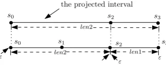
r1, . . . , rh. For example, ⟨s0, s1, s2, s3⟩ ↓ (0,2,2,2,3) =
⟨s0, s2, s3⟩. As depicted in Figure 2, the projected interval
⟨s0, s2, s3⟩can be obtained by using ↓ operator to take the
endpoints of each processε, len(2), ε, ε, len(1).
s0 s1 s2 s3
ε len2
len1 ε
s0 s2 s3
len2
the projected interval
ε
Fig. 2. A projected interval.
An interpretation for a PPTL formula is a tuple I = (σ, i, k, j), where σ is an interval, i, k are integers, and j an integer orω such thati ≤k≼j. Intuitively, (σ, i, k, j)
means that a formula is interpreted over a subintervalσ(i,..,j)
with the current state being sk. The satisfaction relation
(|=) between interpretation I and formula Q is inductively defined as follows.
1) I |=πiffsk[π] =true
2) I |=¬QiffI2Q
3) I |=Q1∧Q2 iffI |=Q1 andI |=Q2
4) I |=⃝Qiffk < j and(σ, i, k+ 1, j)|=Q
5) I |= (Q1, . . . , Qm)prj Q iff there are k = r0 ≤
r1≤. . .≤rm≼j such that (σ, i, r0, r1)|=Q1 and (σ, rl−1, rl−1, rl) |= Ql for all 1 < l ≤ m and (σ′,0,0,|σ′|)|=Qfor σ′ given by:
(a)rm< j andσ′=σ↓(r0, . . . , rm)·σ(rm+1,..,j) (b) rm =j andσ′ =σ↓ (r0, . . . , rh) for some 0 ≤
h≤m.
6) I |= Q+ iff there are finitely many r0, . . . , rn and
k=r0≤r1≤. . .≤rn−1≼rn =j (n≥1)
such that (σ, i, r0, r1)|=Qand (σ, rl−1, rl−1, rl)|=
[image:2.595.380.542.422.487.2]j = ω and there are infinitely many integers k =
r0 ≤ r1 ≤ r2 ≤ . . . such that lim
i→∞ri = ω and (σ, i, r0, r1)|=Q and for l > 1,(σ, rl−1, rl−1, rl) |=
Q.
A PPTL formulaQ is satisfied by an intervalσ, denoted by σ |= Q, if (σ,0,0,|σ|) |= Q. A formula Q is called satisfiable, if σ |= Q. A formula Q is valid, denoted by |=Q, if σ|=Q for allσ. Sometimes, we denote|=p↔q (resp. |= p → q) by p ≈ q (resp.,→ ) and |= 2(p ↔ q)
(resp. |= 2(p → q)) by p ≡ q (resp. p ⊃ q), The former is calledweak equivalence (resp. weak implication) and the latterstrong equivalence (resp. strong implication).
Figure 3 below shows us some useful formulas derived from elementary PTL formulas. ε represents the final state andmore specifies that the current state is a non-final state; 3P (namely sometimes P) means that P holds eventually in the future including the current state;2P (namelyalways
P) represents thatPholds always in the future from now on;
⊙
P (weak next) tells us that either the current state is the final one orP holds at the next state of the present interval;
Prj(P1, . . . , Pm) represents a sequential computation of
P1, . . . , Pm since the projected interval is a singleton; and
P ;Q(P chopQ) represents a computation of P followed byQ, and the intervals forP andQshare a common state. That is, P holds from now until some point in future and from that time point Q holds. Note thatP ;Q is a strong chop which always requires that P be true on some finite subinterval.len(n)specifies the distancenfrom the current state to the final state of an interval; skip means that the length of the interval is one unit of time.fin(P)is true as long asPistrueat the final state whilekeep(P)istrueifP is true at every state but the final one. The formulahalt(P)
holds if and only if formula P istrue at the final state.
ε def= ¬ ⃝true
len(n) def= {
ε ifn= 0
⃝len(n−1) ifn >1
2P def= ¬3¬P
skip def= len(1)
Prj(P1, . . . , Pm) def
= (P1, . . . , Pm)prj ε
fin(P) def= 2(ε→P)
P ;Q def= Prj (P, Q)
keep(P) def= 2(¬ε→P)
more def= ¬ε
halt(P) def= 2(ε↔P)
3P def= Prj(true, P)
⊙
[image:3.595.57.276.480.669.2]P def= ε∨ ⃝P
Fig. 3. Derived PPTL formulas.
An Application of Projection Construct:
Example 1: We present a simple application of projection construct about a pulse generator for variable x which can assume two values: 0 (low) and 1 (high).
We first define two types of processes: The first one is hold(i)which is executed over an interval of length i and ensures that the value of x remains constant in all but the
final state,
hold(i)def= frame(i)∧len(i)
The other isswitch(j)which is ensures that the value of xis first set to 0 and then changed at every subsequent state,
switch(j)def= x= 0∧len(j)∧2(more→ ⃝x= 1−x)
Having definedhold(i)andswitch(j), we can define the pulse generators with varying numbers and length of low and high intervals forx,
pulse(i1, . . . , ik) def
= (hold(i1), . . . , hold(ik))prj switch(k)
LetQbe a PPTL formula andQp∈AP be a set of atomic
propositions in Q. Normal form of PPTL formulas can be defined as follows.
Definition 2: A PPTL formulaQis innormal formif
Q≡( n0 ∨
j=0
Qej ∧ε)∨( n ∨
i=0
Qci∧ ⃝Qfi)
whereQej ≡ m∧0
k=1 ˙
qjk, Qci ≡ m ∧ h=1
˙
qih,|Qp|=l,1≤m0≤l, 1≤m≤l;qjk, qih ∈Qp, for anyr∈Qp,r˙meansror¬r;
Qf i is a general PPTL formula. For convenience, we often
writeQe∧εinstead of n∨0
j=0
Qej∧εand n ∨
i=0
Qi∧⃝Q′iinstead
of
n ∨
i=0
Qci∧ ⃝Qfi. Thus,
Q≡(Qe∧ε)∨( n ∨
i=0
Qi∧ ⃝Q′i)
whereQe andQi are state formulas.
Theorem 1: For any PPTL formula Q, there is a normal formQ′ such that Q≡Q′. [12]
III. PROBABILISTICSYSTEM
We model probabilistic system by(discrete-time) Markov chains(DTMC). Without loss of generality, we assume that a DTMC has a unique initial state.
Definition 3: A Markov chain is a tuple M = (S,Prob, ιinit, AP, L), whereSis a countable, nonempty set
of states;Prob :S×S →[0,1]is the transition probability function such that ∑
s′∈S
Prob(s, s′) = 1; ιinit :S →[0,1]is
the initial distribution such that ∑
s∈S
ιinit(s) = 1, andAP is
a set of atomic propositions and L : S → 2AP a labeling
function.
As in the standard theory of Markov processes [8], we need to formalize a probability space of M that can be defined as ψM = (Ω,Cyl, P r), where Ω denotes the set
of all infinite sequences of states ⟨s0, s1, . . .⟩ such that Prob(si, si+1) > 0 for all i ≤ 0, Cyl is a σ-algebra
generated by thebasic cylindric sets:
Cyl(s0, . . . , sn) ={path∈Ω|path=s0, s1, . . . , sn, . . .}
andP r is a probability distribution defined by
P rM(Cyl(s0, . . . , sn)) = Prob(s0, . . . , sn)
= ∏
0≤i<n
If p is a path in DTMC M and Q a PPTL formula, we often write p|=Q to mean that a path in DTMC satisfies the given formulaQ. Letpath(s)be a set of paths in DTMC starting with state s. The probability for Qto hold in state s is denoted by P rM(s |= Q), where P rM(s |= Q) =
P rM
s {p∈path(s)|p|=Q}.
IV. PROBABILISTICMODELCHECKING FORPPTL In [12], it is shown that any PPTL formulas can be rewrit-ten into normal form, where a graphic description for normal form called Normal Form Graph (NFG) is presented. NFG is an important basis of decision procedure for satisfiability and model checking for PPTL. In this paper, the work reported depends on the NFG to investigate the probabilistic model checking for PPTL.
However, there are some differences on NFG between our work and the previous work in [10], [11], [12]. First, NFG consists of finite paths and infinite paths. For concurrent stochastic systems, we only consider to verify ω-regular properties. Thus, we are supposed to concern with all the infinite paths of NFG. These infinite paths are denoted by
NFGinf. Further, to define the nodes which recur for finitely
many times, [12] uses Labeled NFG (LNFG) to tag all the nodes in finite cycles withF. But it can not identify all the possible acceptance cases. As the standard acceptance con-ditions inω-automata, we adopt Rabin acceptance condition to precisely define the infinite paths inNFGinf. In addition,
since Markov chainM is a deterministic probabilistic model, in order to guarantee that the product ofM⊗NFGinf is also
a Markov chain, theNFGinf needs to be deterministic. Thus,
following the Safra’s construction for deterministic automata, we design an algorithm to obtain a deterministicNFGinf.
A. Normal Form Graph
In the following, we first give a general definition of NFG for PPTL formulas.
Definition 4 (Normal Form Graph [10], [12]): For a PPTL formula P, the set V(P) of nodes and the set of E(P) of edges connecting nodes in V(P) are inductively defined as follows.
1) P∈V(P);
2) For all Q ∈ V(P)/{ε,false}, if Q ≡ (Qe∧ε)∨ (
n ∨ i=0
Qi∧ ⃝Q′i), thenε∈V(P),(Q, Qe, ε)∈E(P);
Q′i∈V(P),(Q, Qi, Qi′)∈E(P)for alli,1≤i≤n.
The NFG of PPTL formula P is the directed graph G = (V(P), E(P)).
A finite path for formulaQin NFG is a sequence of nodes and edges from the root to nodeε. while an infinite path is an infinite sequence of nodes and edges originating from the root.
Theorem 2 (Finiteness of NFG): For any PPTL formula P,|V(P)| is finite [12].
Theorem 2 assures that the number of nodes in NFG is finite. Thus, each satisfiable formula of PPTL is satisfiable by a finite transition system (i.e., finite NFG). Further, by the finite model property, the satisfiability of PPTL is decidable. In [12], Duanetalhave given a decision procedure for PPTL formulas based on NFG.
To verify ω-regular properties, we need to consider the infinite paths in NFG. By ignoring all the finite paths, we can obtain a subgraph only with infinite paths, denotedNFGinf.
Definition 5: For a PPTL formulaP, the set Vinf(P) of
nodes and the set ofEinf(P)of edges connecting nodes in
Vinf(P)are inductively defined as follows.
1) P ∈Vinf(P);
2) For allQ∈Vinf(P), ifQ≡(Qe∧ε)∨( n ∨ i=0
Qi∧⃝Q′i),
then Q′i ∈ Vinf(P), (Q, Qi, Q′i) ∈Einf(P) for all i, 1≤i≤n.
Thus, NFGinf is a directed graph G′ = (Vinf(P), Einf(P)). Precisely, G′ is a subgraph of G
by deleting all the finite path from nodeP to nodeε. In fact, a finite path in the NFG of a formula Q cor-responds to a model (i.e., interval) of Q. However, the result does not hold for the infinite case since not all of the infinite paths in NFG can be the models of Q. Note that, in an infinite path, there must exist some nodes which appear infinitely many times, but there may have other nodes that can just recur for finitely many times. To capture the precise semantics model of formulaQ, we make use of Rabin acceptance condition as the constraints for nodes that must recur finitely.
Definition 6: For a PPTL formula P, NFGinf with
Rabin acceptance condition is defined as GRabin = (Vinf(P), Einf(P), v0,Ω), where V(P) is the set of nodes
andE(P)is the set of directed edges betweenV(P),v0∈
V(P)is the initial node, and Ω ={(E1, F1), . . . ,(Ek, Fk)}
withEi, Fi ∈V(P)is Rabin acceptance condition. We say
that: an infinite path is a model of the formula P if there exists an infinite runρon the path such that
∃(E, F)∈Ω.(ρ∩E=∅)∧(ρ∩F ̸=∅)
Example 2: Let Q be PPTL formulas. The normal form of3Qare as follows.
3Q ≡ true;Q
≡ (ε∨ ⃝true);Q ≡ (ε;Q)∨(⃝true ;Q)
≡ Q∨ ⃝(true;Q)
≡ (Q∧ε)∨(Q∧ ⃝true)∨ ⃝3Q ≡ (Q∧ε)∨(Q∧ ⃝(ε∨ ⃝true))∨ ⃝3Q
The NFG and NFGinf with Rabin acceptance condition
of3Qare depicted in Figure 4. By the semantics of formula 3Q(see Figure 3), that is, formulaQholds eventually in the future including the current state, we can know that node3Q must cycle for finitely many times and node T (i.e., true) for infinitely many times.
B. The Algorithms
To investigate the probabilistic model checking problem for interval-based temporal logics, we use Markov chainM as stochastic models and PPTL as a specification language. In the following, we present algorithms for the construction and determinization ofNFGinf with Rabin acceptance condition
ε Q
♦Q T
ε
T T
T Q
♦Q T
T T Q
(i) NFG of♦Q. (ii)NFGinf of♦Q.
⇒ ⇒
(iii)NFGinf with Rabin acceptance condition of♦Q. ♦Q
T
T T Q
[image:5.595.139.456.132.622.2]where Ω ={(♦Q, T)}.
Fig. 4. NFG of3Q.
TABLE I
ALGORITHM FOR CONSTRUCTINGNFGinfWITHRABIN CONDITION FOR APPTLFORMULA.
FunctionNFGinf(Q)
/*precondition: Q is a PPTL formula, NF(Q) is the normal form forQ*/ /*postcondition:NFGinf(Q)outputsNFGinf with Rabin condition ofQ,
GRabin= (Vinf(Q), Einf(Q), v0,Ω)*/ begin function
Vinf(Q) ={Q};Einf(Q) =∅;visit(Q) = 0;v0=Q;E=F=∅; /*initialization*/ whilethere existsR∈Vinf(Q)andvisit(R) == 0
doP =NF(R); visit(R) = 1;
switch(P)
caseP≡
h ∨ j=1
Pej∧ε:break;
caseP≡
k ∨ i=1
Pi∧ ⃝Pi′orP ≡( h ∨ j=1
Pej∧ε)∨( k ∨ i=1
Pi∧ ⃝Pi′):
foreachi(1≤i≤k)do
if ¬(Pi′≡false) andPi′̸∈Vinf(Q)
then visit(Pi′) = 0;
/*Piis not decomposed to normal form*/
Vinf(Q) =Vinf(Q)∪
k ∪ i=1{
Pi′};
Einf(Q) =Einf(Q)∪
k ∪ i=1{
(R, Pi, Pi′)};
if¬(Pi′≡false) andPi′∈Vinf(Q)
thenEinf(Q) =Einf(Q)∪
k ∪ i=1{
(R, Pi, Pi′)};
whenPi′=R do /*self-loop*/
ifRisQ1;Q2 thenE=E∪ {R}elseF=F∪ {R} forsome nodeR′′∈Vinf(Q);
letN F(R′′) =
k ∨ j=1
Ri∧ ⃝Ror
N F(R′′) = (
h ∨ j=1
Rej∧ε)∨( k ∨ i=1
Ri∧ ⃝R);
/*nodesRandR′′form a loop*/
whenPi′=R′′(R′′̸=R)do
ifR, R′′̸∈EthenF=F∪ {{R, R′′}} elseE=E∪ {{R, R′′}};
break;
end while returnGRabin;
end function
Construction of NFGinf : In Table I, we present
algo-rithm NFGinf(Q) for constructing the NFGinf with
Ra-bin acceptance condition for any PPTL formula. Algorithm
NF(Q)can be found in [12], which is used for the purpose of transforming formula Q into its normal form. For any formula R ∈ Vinf(Q) and visit(R) = 0, we assume that
P =NF(R)is in normal form, where visit(R) = 0 means that formula R has not been decomposed into its normal form. When P ≡ ∨ki=1Pi ∨ ⃝Pi′ or P ≡ (
∨h
j=1Pej ∧
ε)∨(∨ki=1Pi∧ ⃝Pi′), ifPi′ is a new formula (node), that
is, Pi′ ̸∈ Vinf, then by Definition 5, we add the new node
Pi′ to Vinf and edge (R, Pi, Pi′) to Einf respectively. On
the other hand, if Pi′ ∈ Vinf, then it will be a loop. In
particular, we need to consider the case of R ≡Q1 ; Q2.
BecauseQ1 ;Q2 (Q1chopQ2, defined in Fig.3) represents
a computation of Q1 followed by Q2, and the intervals for
Q1 and Q2 share a common state. That is, Q1 holds from
now until some point in future and from that time pointQ2
holds. Note thatQ1 ;Q2 used here is a strong chopwhich
always requires thatQ1 be true on some finite subinterval.
Therefore, infinite models ofQ1 can causeRto be false. To
constraint that chop formula will not be repeated infinitely many times.
By Theorem 2, we know that nodes V(Q) is finite in
NFG. SinceVinf(Q)⊆V(Q), soVinf(Q)is finite as well.
This is essential since it can guarantee that the algorithm
NFGinf(Q)will terminate.
Theorem 3: AlgorithmNFGinf(Q)always terminates.
Proof:LetVinf(Q) ={v1, . . . , vn}. When all nodes inVinf
are transformed into normal form, we have visit(vi) == 1 (1≤i≤n). Hence, the while loop always terminates.
We denote the set of infinite paths in an NFGinf G by
path(G) = {p1, . . . , pm}, where pi (1 ≤ i ≤ m) is an
infinite path from the initial node to some acceptable node inF. The following theorem holds.
Theorem 4: GRabinandG′Rabinare equivalent if and only
if path(GRabin) =path(G′Rabin).
Let Q be a satisfiable PPTL formula. By unfolding the normal form of Q, there is a sequence of formulas ⟨Q, Q1, Q′1, Q2, Q′2, . . .⟩. Further, by algorithmNFGinf, we
can obtain an equivalentNFGinf to the normal form. In fact,
an infinite path inNFGinf of Qcorresponds to a model of
Q. We conclude this fact in Theorem 5.
Theorem 5: A formula Q can be satisfied by infinite models if and only if there exists infinite paths in NFGinf
of Qwith Rabin acceptance condition.
Determinization ofNFGinf: Buchi automata andNFGinf
both acceptω-words. The former is a basis for the automata-theoretic approach for model checking with liner-time tem-poral logic, whereas the latter is the basis for the satisfia-bility and model checking of PPTL formulas. Following the thought of the Safra’s construction for deterministic Buchi automata [15], we can obtain a deterministic NFGinf with
Rabin acceptance condition from the non-deterministic ones. However, different from the states in Buchi automata, each node in NFGinf is specified by a formula in PPTL. Thus,
by eliminating the nodes that contain equivalent formulas, we can decrease the number of states in the resulting deterministicNFGinf to some degree.
[image:6.595.305.549.67.360.2]The construction for deterministic NFGinf is shown in
Table II. For any R∈Vinf′ (Q),Ris a Safra tree consisting of a set of nodes, and each node v is a set of formulas. By Safra’s algorithm [15], we can compute all reachable Safra tree R′ that can be reached from R on input Pi. To
obtain a deterministicNFGinf, we take all pairs(Ev, Fv)as
acceptance component, whereEv consists of all Safra trees
without a nodev, andFvall Safra trees with nodevmarked
’!’ that denotesvwill recur infinitely often. Furthermore, we can minimize the number of states in the resulting NFGinf
by finding equivalent nodes. Let R = {v0, . . . , vn} and
R′={v0′, . . . , vn′}be two Safra’s trees, whereR, R′ ∈Vinf′ , nodes vi = {Q1, Q2, . . .} and v′i ={Q′1, Q′2, . . .} be a set
of formulas. For any nodes vi andv′i, if we have vi =vi′,
then the two Safra’s trees are the same. Moreover, we have vi =v′i if and only if
∨n
j=1Qj ≡ ∨n
j=1Q′j.
C. Product Markov Chains
Definition 7: Let M = (S,Prob, ιinit, AP, L) be a
Markov chain M, and for PPTL formula Q, GRabin = (Vinf(Q), Einf(Q), v0,Ω)be a deterministicNFGinf, where
TABLE II
ALGORITHM FORDETERMINISTICNFGinf.
FunctionDNFG(Q)
/*precondition:GRabin= (Vinf(Q), Einf(Q), v0,Ω)is anNFGinf for PPTL formulaQ. */
/*postcondition: DNFG(Q) outputs a deterministicNFGinf and
G′Rabin= (Vinf′ (Q), Einf′ (Q), v′0,Ω′)*/ begin function
/*initialization*/
Vinf′ (Q) ={Q};Einf′ (Q) =∅;v′0=v0;Ev=Fv=∅;
whileR∈Vinf′ (Q)and there exists an inputPido
foreachnodev∈Rsuch thatR∩F ̸=∅ dov′=v∩F;R′=R∪ {v′};
foreachnodevinR′
dov={Pi′∈Vinf(Q)| ∃(P, Pi, Pi′)∈Einf(Q), P∈v};
/*updateR′*/
foreachv∈R′do ifPi∈vsuch thatPi∈left sibling ofv
thenremovePiinv;
foreachv∈R′do ifv=∅thenremovev;
foreachv∈R′do ifu1, . . . , unare all sons ofv
such thatv=∪i{ui} thenremoveui; markvwith!;
Vinf′ (Q) ={R′} ∪Vinf′ (Q);Einf′ (Q) = (R, Pi, R′)∪E′inf(Q);
end while
/*Rabin acceptance components*/
Ev={R∈Vinf′ (Q)|R is Safra tree without nodev};
Fv={R∈Vinf′ (Q)|R is Safra tree withvmarked!};
returnG′Rabin;
end function
Ω ={(E1, F1), . . . ,(Ek, Fk)}. The productM ⊗GRabin is
the Markov chain, which is defined as follows.
M ⊗GRabin = (S×Vinf(Q),Prob′, ιinit,{acc}, L′)
where
L′(⟨s, Q′⟩) =
{acc} if for someFi, Q′∈Fi,
andQ′ ̸∈Ej for allEj, 1≤i, j≤k
∅ otherwise
ι′init(⟨s, Q′⟩) = {
ιinit if (Q, L(s), Q′)∈Einf 0 otherwise
and transition probabilities are given by
Prob′(⟨s′, Q′⟩,⟨s′′, Q′′⟩)
= {
Prob(s′, s′′) if(Q′, L(s′′), Q′′)∈Einf
0 otherwise
A bottom strongly connected components (BSCCs) inM⊗ GRabin is accepting if it fulfills the acceptance conditionΩ
inGRabin.
For some states∈M, we need to compute the probability for the set of paths starting fromsinM for whichQholds, that is, the value ofP rM(s|=Q). From Definition 7, it can
be reduced to computing the probability of accepting runs in the product Markov chainM⊗GRabin.
Theorem 6: Let M be a finite Markov chain,sa state in M,GRabin a deterministic NFGinf for formula Q, and let
U denote all the accepting BSCCs inM⊗GRabin. Then, we
have
P rM(s|=GRabin) =P rM⊗GRabin(⟨s, Q′⟩ |=3U)
Corollary 7: All the ω-regular properties specified by PPTL are measurable.
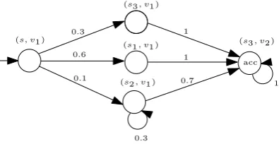
Example 3: We now consider the example in Figure 1. LetM denote Markov chain in Figure 1(b). The probability thatsequential propertyp;qholds in Markov chainM can be computed as follows.
First, by the two algorithms above, deterministicNFGinf
with Rabin condition for p ; q is constructed as in Figure 1(a), where the Rabin acceptance condition isΩ = (v1, v2).
Further, the product of the Markov chain and NFGinf for
formula p;q is given in Figure 5.
(s, v1 )
(s3, v1 )
(s1, v1 )
(s2, v1 )
(s3, v2 )
0.3 1
1 0.6
0.1 0.7
0.3
[image:7.595.73.271.199.301.2]1 acc
Fig. 5. The Product of Markov chain andNFGinf in Figure 1.
From Figure 5, we can see that state(s3, v2)is the unique
accepting BSCC. Therefore, we have P rM(s|=G
Rabin) = P rM⊗GRabin((s, v
1)|=3(s3, v2))
= 1
That is, sequential property p; q is satisfied almost surely by the Markov chain M in Figure 1(b).
V. CONCLUSIONS
This paper presents an approach for probabilistic model checking based on PPTL. Both propositional LTL and PPTL can specify linear-time properties. However, unlike proba-bilistic model checking on propositional LTL, our approach uses NFGs, not Buchi automata, to characterize models of logic formulas. NFGs possess some merits that are more suitable to be employed in model checking for interval-based temporal logics.
Recently, some promising formal verification techniques based on NFGs have been developed, such as [13], [14]. In the near future, we will extend the existing model checker for PPTL with probability, and according to the algorithms proposed in this paper, to verify the regular safety properties in probabilistic systems.
REFERENCES
[1] H. Hansson and B. Jonsson. (1994), A Logic for Reasoning about Time and Reliability. Formal Aspects of Computing. Vol. 6, pages 102-111. [2] A. Aziz, K. Sanwal, V. Singhal and R. K. Brayton. (2000), Model Checking Continous Time Markov Chains. ACM Trans. Comput. Log. Vol. 1(1): 162-170.
[3] B. Moszkowski. (1983), Reasoning about digital circuits. PhD Thesis. Stanford University. TRSTAN-CS-83-970.
[4] B.Moszkowski. (1986), Executing temporal logic programs. Cambridge University Press.
[5] M. Z. Kwiatkowska, G. Norman and D. Parker. (2004), Probabilistic Symbolic Model Checking with PRISM: a hybrid approach.STTT. Vol. 6(2): 128-142.
[6] C. Baier, J. P. Katoen. (2008), Principles of Model Checking. The MIT Press.
[7] J. -P. Katoen, M. Khattri and I. S. Zapreev. (2005), A Markov Reward Model Checker. InQEST, pages 243-244.
[8] J. G. Kemeny and J. L. Snell. (1960), Finite Markov Chains. Van Nostrad, Princeton.
[9] P. L. Wolper. (1983), Temporal logic can be more expressive.
Informa-tion and Control, vol.56, pages 72-99. 1983.
[10] Z.Duan, X.Yang and M.Koutny. (2008), Framed Temporal Logic Programming.Science of Computer Programming, Volume 70(1), pages 31-61, Elsevier North-Holland.
[11] X. Yang and Z. Duan. (2008) Operational Semantics of Framed Tempura.Journal of Logic and Algebraic Programming, Vol.78(1):22-51, Elsevier North-Holland.
[12] Z. Duan, C. Tian, L. Zhang. (2008), A Decision Procedure for Propositional Projection Temporal Logic with Infinite Models. Acta
Informatic, Springer-Verlag, 45, 43-78.
[13] C.Tian and Z. Duan. (2010), Making Abstraction Refinement Efficient in Model Checking CoRR abs/1007.3569.
[14] C. Tian, Z. Duan. (2007), Model Checking Propositional Projection Temporal Logic Based on SPIN. ICFEM pages: 246-265.