High spatial resolution galactic 3D extinction mapping with IPHAS

University of Warwick institutional repository: http://go.warwick.ac.uk/wrap

This paper is made available online in accordance with

publisher policies. Please scroll down to view the document

itself. Please refer to the repository record for this item and our

policy information available from the repository home page for

further information.

To see the final version of this paper please visit the publisher’s website.

Access to the published version may require a subscription.

Author(s): Stuart E. Sale, J. E. Drew, Y. C. Unruh, M.J. Irwin, C.

Knigge, S. Phillipps, A. A. Zijlstra, B. T. Gänsicke, R. Greimel, P. J.

Groot, A. Mampaso, R. A. H. Morris, R. Napiwotzki, D. Steeghs, N. A.

Walton

Article Title:

High spatial resolution Galactic 3D extinction mapping with

IPHAS

Year of publication: 2009

Link to published article:

arXiv:0810.2547v1 [astro-ph] 14 Oct 2008

High Spatial Resolution Galactic 3D Extinction Mapping with

IPHAS

Stuart E. Sale

1

⋆

, J. E. Drew

1

,

2

, Y. C. Unruh

1

, M.J. Irwin

3

, C. Knigge

4

, S. Phillipps

5

,

A. A. Zijlstra

6

, B. T. G¨ansicke

7

, R. Greimel

8

, P. J. Groot

9

, A. Mampaso

10

,

R. A. H. Morris

5

, R. Napiwotzki

2

, D. Steeghs

7

,

11

N. A. Walton

3

4_{School of Physics & Astronomy, University of Southampton, Southampton, SO17 1BJ, U.K.}

5_{Astrophysics Group, Department of Physics, Bristol University, Tyndall Avenue, Bristol, BS8 1TL, U.K.}

6_{Jodrell Bank Center for Astrophysics, Alan Turing Building, The University of Manchester, Oxford Street, Manchester, M13 9PL, U.K.} 7_{Department of Physics, University of Warwick, Coventry, CV4 7AL, U.K.}

8_{Institut f¨ur Physik, Karl-Franzens Universit¨at Graz, Universit¨atsplatz 5, 8010 Graz, Austria}

9_{Department of Astrophysics/IMAPP, Radboud University Nijmegen, P.O. Box 9010, 6500 GL, Nijmegen, The Netherlands} 10_{Instituto de Astrof´ısica de Canarias, Via L´actea s/n, E38200 La Laguna, Santa Cruz de Tenerife, Spain}

11_{Harvard-Smithsonian Center for Astrophysics, 60 Garden Street, Cambridge, MA 02138, USA}

Received ..., Accepted...

ABSTRACT

We present an algorithm (MEAD, for ‘Mapping Extinction Against Distance’) which will de-termine intrinsic (r′₋i′) colour, extinction, and distance for early-A to K4 stars extracted from the IPHAS r′/i′/Hαphotometric database. These data can be binned up to map extinction in three dimensions across the northern Galactic Plane. The large size of the IPHAS database (_∼200 million unique objects), the accuracy of the digital photometry it contains and its faint limiting magnitude (r′_∼20) allow extinction to be mapped with fine angular (_∼10 arcmin) and distance (_∼0.1 kpc) resolution to distances of up to 10 kpc, outside the Solar Circle. High reddening within the Solar Circle on occasion brings this range down to_∼2 kpc. The resolution achieved, both in angle and depth, greatly exceeds that of previous empirical 3D extinction maps, enabling the structure of the Galactic Plane to be studied in increased detail. MEADaccounts for the effect of the survey magnitude limits, photometric errors, unresolved ISM substructure, and binarity. The impact of metallicity variations, within the range typical of the Galactic disc is small. The accuracy and reliability of MEAD are tested through the use of simulated photometry created with Monte-Carlo sampling techniques. The success of this algorithm is demonstrated on a selection of fields and the results are compared to the literature.

Key words: surveys – methods: miscellaneous – ISM: dust, extinction – ISM: structure – Galaxy: disc – stars: general

1 INTRODUCTION

The INT/WFC Photometric Hα Survey of the northern Galactic Plane (IPHAS; Drew et al. 2005) is the first comprehensive digital survey of the disc of the Galaxy (|b|65◦), north of the celestial equator. Imaging is performed in the r′, i′and Hαbands down to r′∼20 (10σ). The high quality photometry from this survey has been shown to enable early-A type stars to be selected very easily, due to their strong Hαabsorption (Drew et al. 2008). In this same

⋆ _{E-mail: [email protected]}

study, the(r′−i′)colours provided by IPHAS were used to deter-mine the extinctions of the A stars selected, and then distances were deduced using photometric parallax. This capability is a specific example of a more general property of the IPHAS: since(r′−Hα)

The IPHAS catalogue contains high quality photometry for

∼200 million objects, equating to over 105objects per square de-gree. Our analysis of a wide variety of IPHAS fields has shown that the data quality allows for accurate determinations of distances and extinctions to the studied objects, with median errors of typically

∼100pc on distance and approximately 0.1 magnitudes of error on the determined extinction. The limiting magnitude of the IPHAS catalogue (r′∼20,10σ) is sufficient for extinctions to be measured to distances up to∼10 kpc from the Sun.

Juri´c et al. (2008) discuss and demonstrate the potential for accurate wide area surveys in analysing the structure of the Milky Way. They utilise the Sloan Digital Sky Survey (SDSS) in order to determine the stellar number density distribution mostly at Galac-tic latitudes |b|>25o. As a result of this they are able to eas-ily study the Galactic halo and local scale heights of the Milky Way’s thick and thin discs, and find localised over-densities. In contrast the IPHAS survey area covers low Galactic latitudes, en-abling the Galactic thin disc to be studied in detail, well beyond the solar neighbourhood. The cost associated with this is that ex-tinction, which is largely negligible in the SDSS survey area, be-comes a significant concern to the extent that understanding its three-dimensional (3D) distribution is a necessary hurdle that must be overcome on the path to studying the structure of the Galactic disc.

Applications of extinction mapping go beyond studies of Galactic structure: a distance-extinction relationship, combined with an estimate of the extinction to an object has often been ex-ploited to give an estimate of the distance to individual objects. Such estimates are of particular use for objects such as planetary nebulae, for which reliable estimates of distance are difficult to ob-tain (Viironen et al. in preparation).

There is a long history associated with trying to map the dis-tribution of extinction, going back as far as Trumpler (1930) and van de Kamp (1930) who both appreciated that extinction is con-centrated near the Galactic plane. Subsequent efforts to map ex-tinction can be broken down into two broad categories: 2D maps of the asymptotic extinction and 3D maps with varying degrees of model input.

Several studies have produced 2D maps of the maximum asymptotic extinction over the sky. Burstein & Heiles (1982) used HI mapping and galaxy counts, estimating the errors in derived ex-tinctions to be∼10%. Schlegel, Finkbeiner & Davis (1998) pro-vided updated maps based on COBE and FIRAS measurements of dust emission at 100µm. The Schlegel et al. (1998) maps have since been widely used, but they warn that their values for|b|<5◦are subject to significant errors, an assertion that has been supported by Arce & Goodman (1999) and Cambr´esy, Jarrett & Beichman (2005). More recently Froebrich et al. (2005) have used cumulative star counts from the 2MASS survey to construct a 2D extinction map of the Galactic plane (|b|<20◦).

3D extinction models have grown progressively more sophis-ticated, moving from the simple cosecant model (Parenago 1945) to the modern, high resolution models of Mendez & van Altena (1998); Chen et al. (1999); Drimmel & Spergel (2001) and Amˆores & L´epine (2005). Marshall et al. (2006) compared the Besanc¸on Galactic model (Robin et al. 2003), without extinction, to 2MASS (Two Micron All-Sky Survey) observations. The dif-ferences between the observed and theoretical colours of predomi-nantly K & M giants were then attributed to extinction. This semi-empirical method is able to map extinction at fine angular resolu-tions (0.25◦_×0.25◦).

Historically, attempts to empirically map extinction in three

dimensions have been constrained by the availability and qual-ity of photometric data. Early studies include Fernie (1962); Eggen (1963); Isserstedt & Schmidt-Kaler (1964); Neckel (1966); Scheffler (1966, 1967), all of which reached no fainter than V∼10 and therefore could only cover relatively limited ranges of up to a 1−2 kpc. Also, they all contain fewer than 5000 objects, limit-ing their mapplimit-ings to very coarse spatial resolutions. Furthermore, Fitzgerald (1968) found that these works produced ‘varying, and sometimes apparently conflicting results’. Subsequently, Fitzgerald (1968); Lucke (1978) and Neckel, Klare & Sarcander (1980) con-tinued, with similar approaches, but they were still limited by the available photometric catalogues, with the most recent of the three (Neckel et al. 1980) using a catalogue of∼11,000 objects. As a result, they achieved angular resolutions on the order of a few de-grees.

Here, we present a new approach to mapping the 3D extinction within the plane of our Galaxy, based on IPHAS photometry. The depth, quantity and quality of this data set allows us to construct a new extinction map with high angular (10′) and distance (100 pc) resolution out to very large distances (up to 10 kpc). In the present paper, we focus on the algorithm used to construct this map, leaving the map itself to be presented in a separate publication. The algo-rithm which is used to calculate extinction distance-relationships from IPHAS data (hereafter referred to asMEAD, Mapper of Ex-tinction Against Distance) is discussed in detail in Section 3. In order for it to be used with IPHAS data it is necessary to calibrate this translation of IPHAS photometry into derived quantities (Sec-tion 2). Sec(Sec-tion 4 shows the use of simulated photometry to deter-mine the values of some key parameters used inMEADand demon-strate its accuracy in the face of a range of possible problems. Fi-nally, Section 5, investigates the use ofMEADon real IPHAS data, showing the power of its approach.

2 DECODING INTRINSIC COLOUR, LUMINOSITY

CLASS AND EXTINCTION FROM IPHAS PHOTOMETRY

In order to exploit IPHAS, it is necessary to understand the be-haviour of its colour-colour and colour-magnitude planes – specif-ically the intrinsic colours of normal stars and their response to extinction. To this end Drew et al. (2005) produced simulations of the luminosity class sequences on the IPHAS colour-colour plane using the spectral library of Pickles (1998). In Fig. 1 we provide an example of(r′−Hα,r′−i′)data for a survey field with differ-ently reddened simulated main sequences spanning the O9 to M3 spectral type range superposed: this shows how reddening shifts the main sequence across to the right, creating a lower edge to the main stellar locus that is well-described as the early-A reddening line. Reddening also moves O and B stars to the same colours as A and F stars, though they are still separated in apparent magnitude. For the purpose of emulating the colour behaviour of normal stars, the Pickles (1998) library contains limited numbers of objects that cannot support a full exploration of the available parameter space. In particular, in order to examine the impact of changing metal-licity and fine variations in luminosity class, we have recomputed expected IPHAS colours from grids of model atmospheres.

Figure 1. Black points show data from IPHAS field 4199, where 136r′<

20. Main sequences where extinctions equivalent to AV=0 (red), 4 (green),

8 (blue) for an A0V star have been applied are shown with solid lines and the dashed cyan line shows an A3V reddening line. There are two main populations visible in Fig. 1, the first lies at bluer (r′−i′) aligned with and extending beyond the simulated unreddened main sequence: this population is mainly K-M dwarfs. The main body of stars falls between the AV=4 and

AV=8 main sequences. The long trail of objects stretching from (r′−i′)≈2

are M giants. Finally, there are five objects that appear to lie above the unreddened main sequence, these objects are candidate Hαemitters.

Figure 2. A Hertzsprung-Russell diagram of the simulated luminosity classes used in this study. The unshaded region of the diagram indicates the intrinsic colour range of interest, which is the range of intrinsic colour thatMEADworks on.

only an incomplete sample of diatomic molecules and, with the ex-ception of H2O, no triatomic or larger molecules. This inherently

leads to deviations from reality, which become significant for late K and all M type stars (Bertone et al. 2004). In particular the ab-sence of VO lines means that Kurucz models are not available for Teff<3500K (approximately M4 or later) as they would be

particu-larly inaccurate (Kurucz 2005). Similar problems affect other grids of atmospheres, with the consequence that, for our purposes, there are no reliable alternative model grids at these low temperatures.

Table 1. The intrinsic (r′_−i′_{) and (r}′_{−Hα) colours, and r’ magnitude} com-pared to approximate spectral type and Tefffor solar metallicity dwarfs. The

data are derived from the Straizys & Kuriliene (1981) Teff, log g calibration

and the absolute magnitude calibration of Houk et al. (1997).

Intrinsic Intrinsic r′Absolute Spectral Teff

(r′−i′) (r′−Hα) Magnitude Type

-0.047 0.029 0.12 B8 11510

-0.028 0.013 0.51 B9 10400

-0.006 -0.002 0.80 A0 9600

0.001 -0.005 1.09 A1 9400

0.013 -0.008 1.28 A2 9150

0.025 -0.008 1.47 A3 8900

0.060 0.006 1.84 A5 8400

0.097 0.032 2.21 A7 8000

0.171 0.098 2.64 F0 7300

0.203 0.128 2.92 F2 7000

0.258 0.174 3.37 F5 6500

0.296 0.202 3.83 F8 6150

0.318 0.218 4.11 G0 5950

0.336 0.229 4.39 G2 5800

0.372 0.252 4.75 G5 5500

0.406 0.269 5.21 G8 5250

0.436 0.283 5.58 K0 5050

0.454 0.291 5.76 K1 4950

0.472 0.298 6.04 K2 4850

0.504 0.312 6.20 K3 4700

0.527 0.322 6.48 K4 4600

2.1 Method and underpinning stellar data

So as to use the synthetic spectral libraries to create lu-minosity class sequences, the classes of the MK system (Morgan, Keenan & Kellman 1943) must be linked to Teff, log g

and absolute magnitudes (MV). This study adopts the Teffand log g

calibrations of Straizys & Kuriliene (1981), as well as their abso-lute magnitude calibrations for all classes except dwarfs, for which we use the data of Houk et al. (1997) based on HIPPARCOS paral-laxes. In Table 1 we give the solar-metallicity mapping of intrinsic

(r′−i′)colour onto main sequence absolute magnitude and spec-tral type that we have adopted, while Fig. 2 shows the relevant Hertzsprung-Russell diagram of the five luminosity classes we use. All synthetic colours were determined largely as by Drew et al. (2005), with the modest difference that the atmospheric transmission curve at the INT is included in the calculation, so that the total transmission profile is the product of the atmospheric transmission, CCD response and filter transmission curves.

As IPHAS magnitudes are based on the Vega system, an appropriate spectrum of Vega was required to provide the zero-point flux. So as to match spectral resolution (which is neces-sary to produce accurate Hαmagnitudes) the ATLAS9 Vega model spectrum available via kurucz.harvard.edu was used. This assumes Teff=9550K and log g=3.80. It should be noted that there has

been much debate over which ATLAS9 spectra best fits observa-tions of Vega. For example, Cohen et al. (1992) and Bohlin (2007) argue that the 9400K model (as opposed to the 9550K model used in this work) is better suited. However, the differences in derived colours are small,δ(r′−Hα)≈0.003, so the choice from these two models is of little consequence.

Figure 3. The simulated main (solid black line) and giant (dashed green line) sequences compared to solar metallicity main sequence objects from the Pickles (1998) and STELIB (Le Borgne et al. 2003) libraries (red crosses). As with figure 2, the unshaded region of the diagram indicates the intrinsic colour range of interest, used by MEAD.

(Sordo & Munari 2006, http://web.pd.astro.it/adsd). However, of these only a small proportion cover the wavelength range required and many of those are unsuitable. Once these have been filtered out, the STELIB library (Le Borgne et al. 2003) and the library of Pickles (1998) remain.

2.2 Comparisons between colour sequences from synthetic

and empirical libraries

Fig. 3 compares the Main Sequence derived from the synthetic spectra of Munari et al. (2005), to colours derived from empiri-cal spectra. For most spectral types the results from empiriempiri-cal and synthetic spectra agree well. However, for M-type stars there is some disagreement. This could be a result of difficulties associ-ated with modelling late type stars, as noted earlier. A compari-son was also performed to sequences derived from the MARCS (Gustafsson et al. 2003) and PHOENIX (Brott & Hauschildt 2005) codes. The MARCS library only covers spectral types from early-A to early-K, but it is in excellent agreement with the results ob-tained from Munari et al. (2005). On the other hand, the sequences of Brott & Hauschildt (2005) are significantly different for spectral types later than roughly K4. On further examination the differences are almost entirely limited to behaviour in the Hαband. It is worth noting that Gustafsson et al. (2008) demonstrate that a new version of the PHOENIX code, employing the Kurucz line data, performs considerably better than the version employed here. Therefore it is possible that the discrepancies we encounter will not be present in this newer version.

Bertone et al. (2004) finds the ATLAS9 and PHOENIX mod-els which best fit intrinsic spectra of known type and list the Teffof

the fit. By assuming that the Teffcalibration of Straizys & Kuriliene

(1981) represents the mean temperature for any given class, it is possible to calculate the standard deviation of the residuals of the Bertone et al. (2004) estimates. This is then an estimate of the com-bination of the error on the Straizys & Kuriliene (1981) Teff

calibra-tion and the natural width of each class. However, allowing for this temperature variation makes no measurable difference to our model sequences.

Unfortunately Bertone et al. (2004) do not give the values of

Figure 4. ZAMS from the Pietrinferni et al. (2004) library on the colour-colour plane, where the colour-colours have been determined from the appropriate Munari et al. (2005) models. In black is a ZAMS for [Fe/H]=0, in red a ZAMS for [Fe/H]=−1.00 and in green a ZAMS for [Fe/H]=−1.82.

log g for each fit, so it is not possible to repeat this procedure for surface gravity. However, Munari et al. (2005) suggest that the nat-ural width of each class in surface gravity is∼0.25 dex. Applying this spread results in the luminosity class sequences changing from lines to bands in colour-colour and colour-magnitude space. The majority of objects from the Pickles (1998) and STELIB libraries now fall within these bands. Bertone et al. (2004) also demonstrate that the quality of the best fit to the stars in the empirical libraries it uses, decreases for later types. This behaviour is again attributable to the poorly understood molecular lines, which dominate the spec-tra of late-type stars.

2.3 The impact of rotational broadening

As might be expected, altering the rotational velocity assumed in the models has negligible effect on the colours. This is as varying rotational velocity will only alter the shape of a non-saturated line and will not affect the strength of absorption or emission. Because all the filters used are broad compared to emission or absorption lines, simply altering the line shapes does not change the observed colours. In saturated lines the equivalent width is affected by rota-tional broadening, but Hαis the only atomic line which produces a significant impact on the photometric colours and it does not satu-rate, even in A3V stars where absorption is strongest.

2.4 The impact of metallicity variation

Given that Straizys & Kuriliene (1981) do not consider the effect of metallicity it is clearly not possible to use the sequences based on it to study the effect of metallicity. However, the library of Pietrinferni et al. (2004) does consider it and so is used in this sec-tion. For Munari et al. (2005) models altering metallicity has little effect on IPHAS colour-colour diagrams, a shown by Fig. 4.

Figure 5. ZAMS from the Pietrinferni et al. (2004) library on the colour-magnitude plane, where the colours have been determined from the ap-propriate Munari et al. (2005) models. The top, in black, is a ZAMS for [Fe/H]=0. The curve is lowered with decreasing metallicity, in blue is [Fe/H]=−0.40, red [Fe/H]=−1.00 and at the bottom, in green, is [Fe/H]=−1.82.

Figure 6. Main sequences where extinctions equivalent to AV=0 (black,

left), 4 (red, middle), 8 (green, right) for an A0V star have been applied. The dashed black lines show the loci of A3V (bottom), G5V (middle) and M4V (top) stars under increasing extinction.

Friel et al. (2002) measured metallicities in low Galactic lati-tude open clusters, finding no objects with [Fe/H]<−0.94, whilst Carraro et al. (2007) determine the mean metallicity in the outer disc to be [Fe/H]≃ −0.35. So, observing an object with a metallic-ity below [Fe/H]=−0.5 in IPHAS would be unusual and metallic-ities as low as [Fe/H]=−1.82 would be extremely rare. Therefore, the effect of metallicity variations on absolute magnitude will be relatively small in IPHAS observations. Section 4.8 further exam-ines the impact of undiagnosed metallicity variations.

2.5 Extinction & reddening

It is very important to note that, in the IPHAS colour-colour plane, the reddening vector is at a significant angle with respect to the majority of the main sequence (see Fig. 6). This makes it possible to derive accurate estimates of intrinsic (r′−i′) colour and extinc-tion simultaneously. For colours based on other commonly used

Figure 7. The coefficient br′ against initial (r′ −i′) for the Straizys & Kuriliene (1981) main sequence. Note that the coefficients ar′ and cr′, multiplying the squared and constant terms, are roughly 103 times smaller than br′.

filter sets such as u′g′r′i′z′or JHK, the reddening vector is almost parallel to the main sequence, creating degeneracy in the available (intrinsic colour, extinction) solutions. This property of the IPHAS colour-colour plane is a result of the strong intrinsic (r′−i′) colour sensitivity of the (r′−Hα) colour, whilst its response to reddening is weak compared to that of broad-band colours. The former prop-erty is due to(r′−Hα)being a proxy for the Hαequivalent width, which itself is strongly dependent on intrinsic (r′−i′) colour.

In many applications in astrophysics it is acceptable to treat the ratio RV =AV/E(B−V) as constant across a wide range of

objects, so that extinction can easily be calculated from reddening and vice-versa. However, as pointed out by McCall (2004) this is not in general true, as the extinction integrated across a given broad-band filter is a function of the SED of the observed object and the amount and wavelength dependence of the extinction it has expe-rienced. McCall (2004) suggests that monochromatic measures of extinction should be used, in preference to broadband measures, as they are independent of the observed objects’ SEDs. Following this concept, MEADmeasures a monochromatic extinction at 6250 ˚A (A6250). This is near the effective wavelength of the r′filter in the

INT system (i.e. taking into account the WFC and atmospheric re-sponse). If the intrinsic colour of the observed object is known it will then be possible to convert to and from more commonly-used broadband measures. In this study, we will refer to monochromatic extinctions in discussions of the simulated photometry, while ex-tinctions derived from real data that are compared with the litera-ture will be presented as broadband values, Ar′. The extinction at r′ is preferred to the extinction in the V band for the reasons discussed by Cardelli, Clayton & Mathis (1989). Section 4.10 investigates the ability ofMEADto change between monochromatic and broadband measures of extinction as R is varied. By choosing to normalise the extinction law to a wavelength in the middle of the range studied the systematic error produced by uncertainty in the value of R is minimised.

This work adopts the extinction laws of Fitzpatrick (2004) for the calculation of extinction values in different filters as a function of A6250. Fortunately, this study avoids the problematic UV region

of extinction is well defined by R only. Following Savage & Mathis (1979) and Howarth (1983), we assumed that R=3.1, so as to rep-resent an average Galactic sight-line.

The calibration of the broadband extinctions to A6250 was

performed using the Munari et al. (2005) library to represent the Straizys & Kuriliene (1981) sequences. Fitting was performed by linear regression of a quadratic polynomial to the data, over a range of 06A6250<10, the functions returned, for a band X, are

ex-pressed as follows: AX=aXA2₆₂₅₀+bXA6250+cX.

Fig. 6 demonstrates the effect of extinction on several different spectral types in the (r′- i′,r′- Hα) plane. Despite being cosmeti-cally similar, there are significant differences in the response to ex-tinction of different spectral types. Fig. 7 demonstrates the variation of the coefficient for the leading linear term in the fits. For objects with types in the critical range A3 to K4 (0.056(r′- i′)<0.55) there is a particularly simple linear relation between this fit coeffi-cient and intrinsic (r′-i′) colour, as can also be seen in Fig. 7.

The differing responses to rising extinction of different spec-tral types is illustrated by the extreme examples of A3V and M4V stars: in Fig. 6 these two types limit the plotted (r′- Hα) range of the main sequence. As more extinction is applied, the (r′ - Hα) range spanned shrinks because the A3V star is reddened more quickly in this colour.

3 MEAD: AN ALGORITHM TO DETERMINE

EXTINCTION-DISTANCE RELATIONS

3.1 Concept

The basic principle of this work is that we wish to determine the distance and intervening extinction to a large sample of objects in the IPHAS database. From the observations, we have three ob-served parameters for each object, namely the r′, i′and Hα mag-nitudes, with errors on each. In order to determine the distance to an object by photometric parallax, we must determine its absolute magnitude and extinction. The simplest way to estimate absolute magnitude is to determine the intrinsic colour and luminosity class of the object. Thus for each object we have three parameters we wish to determine (extinction, luminosity class & intrinsic colour) and three observed parameters.

As described in Section 2, it is possible to ascertain the spec-tral class and monochromatic extinction of an object from its po-sition on the colour-colour plane. But, there are two main sources of degeneracy in this process. The first is caused by the fact that reddening tracks for O, B & early A (A0-2) stars intersect those of later A and F stars. This follows from the fact that Hαabsorption peaks in early A stars and(r′−Hα)is strongly correlated with Hα equivalent width (Drew et al. 2005). As discussed in Section 3.3, it transpires that this is not normally a significant source of degener-acy.

The second more important source of degeneracy is luminos-ity class, which has a significant impact on distance determination. Therefore, to estimate an object’s distance, it is necessary for an es-timate of the luminosity class to be determined first. This is, how-ever, not a trivial task, as the different luminosity class sequences behave very similarly on the IPHAS colour-colour plane. We de-cide on the luminosity class of an object as follows. If two ob-jects of identical intrinsic colours, but different absolute magni-tude, are to have the same apparent magnitude the more luminous object must be further away, and is likely to be more heavily red-dened. This reddening contrast creates two sequences in a colour-magnitude diagram, as can be seen in Fig. 8, where a selection of

Figure 8. A colour-magnitude diagram for F5-8 stars, selected by colour, from IPHAS observations of a 10′×10′ box around (l,b) = (101.55,−0.60). The dwarfs can be seen as the sequence to the left, while the giants are seen to the right. Five brighter objects, probably either F bright-giants, or highly reddened late-O or early-B stars are visible to the extreme right, separated from the giant sequence.

Figure 9. A schematic depiction ofMEAD.

3.2 Details of implementation

Fig. 9 outlines an algorithm that realises this principle (named

MEADfor Mapper of Extinction Against Distance). In the remain-der of this section each of the steps inMEADare described.

Extinction, intrinsic colour and distance are determined si-multaneously for all objects in the intrinsic colour range of inter-est given in Figs. 2 and 3. Objects which fall outside this region of the colour-colour plane which could be occupied by objects of the types we are interested in are simply discarded. The discarded objects will include M and late-K type stars, white dwarfs, extra-galactic objects and stars exhibiting Hαemission. At the same time errors on the derived quantities are also propagated from the pho-tometric errors. Although determined at the same time as distance, the estimates of extinction and intrinsic colour are almost indepen-dent of the luminosity class and can be considered to be determined solely from the colour-colour plane: only very small differences arise from the slight differences between the luminosity class se-quences in the colour-colour plane.

The appearance of objects on the extinction-distance plane is complicated by several factors. Firstly, the size of the errors on the estimated values of extinction and distance vary greatly from object to object. Also, these errors are correlated with distance and extinc-tion, as the apparent magnitude of a source becomes fainter with increasing distance or extinction, increased photometric error is to be expected. Finally, because of the finite angular resolution of the fields, there will inevitably be unresolved substructure within the absorbing material in each field analysed, causing an intrinsic and irreducible spread of extinctions at any given distance. These com-plications are dealt with by assuming that extinction at any given distance is modelled by a distribution other than the delta function: a maximum likelihood estimator is used to determine the value of the parameters that describe the distribution. The choice of family of distributions used here is further discussed in Section 4.4.

IPHAS observations are subject to both bright and faint mag-nitude limits. The implication of this is that for an object at a given distance, it will only be observed if its extinction also falls between two limits, and when these limits are approached, the observations will start to become incomplete. This would bias any estimates. The nature of the bias is that as the faint cut-off is approached, only stars viewed through lower extinction remain in the sample, while more extinguished objects are lost. Hakkila et al. (1997) note the disruptive effect that this had on previous studies (Fitzgerald 1968; Neckel et al. 1980; Arenou et al. 1992). Even at the higher angu-lar resolutions treated here this effect continues to be a problem because the interstellar medium is inhomogeneous down to very small scales. Deshpande (2007) demonstrates that variations in the structure of the ISM naturally extend down to at least the scale of tens of AU. Therefore, it is necessary to continue to attend to the magnitude limits in this study, even though significantly finer an-gular resolutions are achievable than those in earlier work.

To deal with this problem, it is necessary to determine which objects could be close to the magnitude limit in distance extinction space, so that they can be excluded when producing an unbiased distance-extinction relationship. To establish which objects are to be excluded, first all the objects are binned in distance to produce a biased extinction-distance relationship, for each bin the mean and intrinsic standard deviation of the extinction is found. Then, for each object the maximum (dmax) and minimum (dmin) distances for

which observations of that type of object would be complete are es-timated. These distances occur where the following two equations are satisfied, where Abright₆₂₅₀(d)and Afaint

6250(d)correspond to the bright

and faint magnitude limits respectively andσ_A¯(d)is the intrinsic

standard deviation of extinction in the relevant bin:

¯

A6250(dmax) +nσ_A¯(dmax) =Afaint6250(d). (1)

¯

A6250(dmin)−nσA¯(dmin) =A bright

6250(d). (2)

If these equations are satisfied at more than one distance, the largest possible value of dminand smallest possible value of dmax

are taken. In equations 1 and 2 the value of n can be altered. Increas-ing it will reduce the chance of the bias affectIncreas-ing the data, at the cost of decreasing the number of objects which are binned to produce the distance-extinction relationship, whilst decreasing it will act in the opposite sense. There is no immediately obvious value to adopt for n and Section 4.5 discusses the use of simulated photometry to find an appropriate value. At the bright end it is assumed that the magnitude range over which observations become incomplete is small, relative to the apparent magnitude sampling, so objects which are closer than dminare simply discarded. In contrast, at the

faint end where the apparent magnitude sampling is much denser, the magnitude range over which observations become incomplete is significant. Therefore the contribution of each object to the dis-tance and extinction estimates is weighted using a sigmoid function as below:

weight= 1

1+es(µ−µmax). (3)

Where µ is the distance modulus of the object in question, µmaxis the distance modulus corresponding to dmaxand s is related

to the distance modulus range over which the sample becomes in-complete. A suitable value of s was found empirically to be 3. This was achieved by fitting a sigmoid to the faint end of histograms of the numbers of objects of a given spectral type against apparent magnitude. By applying this weight, objects which lie well beyond dmax, where the sample is not complete for all expected extinctions,

are given approximately zero weight, whilst those well within dmax

are given a weight of almost one.

A Bayesian classification method is employed to estimate the luminosity class into which each object falls, given the determined distance-extinction relationship, the apparent magnitude of the ob-ject, an estimate of the extinction to the object and an estimate of its intrinsic colour. The luminosity class sequences are assumed to have Gaussian spread in absolute magnitude, with all sequences having equal and constant spread. The classification is made by evaluating the posterior probability that an object belongs to a lu-minosity class, given its extinction, the distance-extinction relation-ship and the absolute magnitude of that class. The choice of the prior used is discussed in Section 4.3.

A threshold probability is imposed, such that when the proba-bilities of all five classes fall below this, the object is removed from consideration in that iteration. This removes objects which do not appear to fit into any of the luminosity classes.

These procedures are put into an iterative structure, as shown in Fig. 9. The sense of the iteration can be summarised as follows: the distance, extinction and intrinsic colour of each object is es-timated; then these determinations are binned to get a distance-extinction relation; this is then used to determine the luminosity class of the objects; and then the distance, extinction and intrinsic colour are estimated again, given the new estimate of luminosity class. The process has shown good convergence in all cases exam-ined so far. In the range of 5-10 iterations are normally required. Convergence is discussed further in Section 4.2.

edge of the main stellar locus in the colour-colour plane. This is used to obtain the first estimate of the luminosity classes of all objects in the field. It is safe to assume that the great majority of objects on this strip are near main sequence, given that early-A gi-ants are not only relatively rare but also exhibit slightly weaker Hαabsorption that lifts them to higher(r′−Hα). This breaks the degeneracy between the different luminosity classes and enables distances to be reliably estimated at the outset (Drew et al. 2008).

When binning the data by distanceMEAD ensures that: the depth of the bin is at least 100 pc; there are at least eight objects in the bin; the total signal to noise in the bin is at least 130.

It should be noted that not all available data in the IPHAS database are used in this algorithm. Only data flagged as either stel-lar or probably stelstel-lar in all three bands by the processing pipeline are accepted, with the remainder discarded straight away (for more details of the data processing see Irwin & Lewis 2001; Drew et al. 2005; Gonz´alez-Solares et al. 2008). As noted already in this sec-tion only a restricted stellar intrinsic colour range is exploited (marked in Figs. 2 and 3): this is due in part to the Houk et al. (1997) calibration ending at K4V and also to the difficulties asso-ciated with modelling the molecular bands in late type-stars (Sec-tion 2). Following Drew et al. (2008), a maximum bright limit of r′=13.5, i′=11.5 and Hα=12.5 is employed to avoid objects that may be saturated in one or more bands. Occasionally when any fainter objects are classified as saturated by the pipeline, the limit will be moved to the apparent magnitude of that object.

3.3 Possible contaminants

MEADassumes that all the objects examined can be described by one of the luminosity class sequences. In practice there are a mi-nority of exotic objects that will not fit into them. Generally such objects are not a problem if they either: have colours which are outside the rangeMEADlooks at or are significantly less frequent than normal objects. The latter argument relies on the statistical na-ture ofMEAD. Although the properties of individual objects may be incorrectly estimated, the intention is thatMEADwill derive the correct extinction-distance relationship given a large enough sam-ple.

As previously mentioned, O and B stars are contaminant ob-jects that may be mistaken for A and F stars. Fortunately, O and B stars are relatively rare, and present only in young populations. In populations older than∼100 Myrs they are essentially absent. So, in large samples, with a mix of ages, we can comfortably as-sume field A and F stars dominate. The circumstance in which this assumption may come undone is in regions of ongoing star for-mation, especially if the stars that will become A and later-type main sequence stars are still in the pre-main-sequence phase. If such objects remain in the minority for their locale, MEAD should recognise their raised luminosity and classify accordingly. If they become the dominant population, then MEAD may misinterpret them. In Section 5.3MEADis tested against IPHAS observations of the Cygnus OB2 association, where such extreme conditions could exist.

The subdwarf sequence occupies a very similar position on the IPHAS colour-colour plane as its dwarf equivalent and as such there is the possibility that subdwarfs may be erroneously identified as dwarfs and used inMEAD. However, in a volume limited sample it is expected that roughly one in every 103 objects would be a subdwarf (Reid et al. 2001). Given the faint absolute magnitudes of subdwarfs relative to the dwarfs, this proportion becomes even lower in the magnitude limited IPHAS catalogue. Furthermore, the

imposition of a threshold probability in the Bayesian luminosity classifier will promptMEADto discard a large proportion of them as they are offset below the main sequence in colour-magnitude space.

Hydrogen atmosphere white dwarfs largely lie outside the main stellar locus, leaving only a minority inside the region of the colour-colour plane searched byMEAD: these objects will be the very coolest and the very hottest white dwarfs. White dwarfs ex-hibit absolute magnitudes approximately in the range 10.r′.15. Given this and the IPHAS magnitude limits, the database cannot contain even unreddened white dwarfs more distant than 1 kpc. It is estimated that there will be 7.6 white dwarfs per square de-gree in the IPHAS sample, representing∼0.01% of all sources. This estimate is based on a detailed model of the Galactic popu-lation of white dwarfs (Napiwotzki 2008) calibrated using the ob-served white dwarf samples of Holberg et al. (2008) and Pauli et al. (2006), reddening is included in an approximate way. Many white dwarfs will be ignored byMEADdue to their colours lying outside the main stellar locus. Of the handful remaining within more will be discarded by the Bayesian luminosity classifier as belonging to a faint sequence.

Extra-galactic sources will also contaminate the catalogue. Resolved galaxies will be flagged by the CASU pipeline as be-ing extended objects and will be ignored byMEAD. In addition, even some small galaxy images will overlap with the very numer-ous stellar images and hence be classified as extended, also remov-ing them from consideration. Nevertheless, some galaxy images will be sufficiently compact to be classified as stellar. Genuinely compact (i.e. physically small) galaxies are rare, contributing about 3% of all low redshift field galaxies down to B≃20 (r′∼19) ac-cording to Drinkwater et al. (1999), who used the all-object (high latitude) spectroscopic survey of Drinkwater et al. (2000). Extrap-olating this another magnitude deeper (i.e. to r′=20), we would still only expect some 40 objects per square degree, which is com-pletely negligible compared to (i.e. 0.02% of) the 200000 stars per square degree in low latitude fields. Of course, at faint limits all galaxies tend to look less and less resolved, resulting in the well known merging of the stellar and galaxy sequences in star/galaxy separation diagrams (e.g. Driver et al. 2003). However, at r′=20 there are around 2000 galaxies per square in total, approximately two thirds of which are in the final magnitude bin (e.g. Driver et al. 1994), so even if we assume that all these could look stellar, this would only represent a 0.7% contamination of the “stars”. In re-gions of high extinction, the counts would, of course, be reduced at given r′. For an asymptotic Ar=2, for instance, the galaxy counts

would be reduced by a factor of about 8, though this would be com-pensated somewhat by the galaxies having smaller angular sizes as the low surface brightness outer parts are too faint to detect (Phillipps, Ellis & Strong 1981). This would reduce the contami-nation to∼200 per square degree or∼0.1%.

Quasars and other distant AGN will also show unresolved images, but again numbers are small. From the Drinkwater et al. (2000) all-object survey, Meyer et al. (2001) find 35 QSOs (of all colours) per square degree to B≃20.2 (r′∼19.5). Given the steep quasar number counts (Croom et al. 2004), this would be_∼70 per square degree at r′=20. Vanden Berk et al. (2005) find a some-what lower number density in the i′ band and many QSOs may have colours too blue to be included in our sample here, so we can estimate a contamination rate of order 0.02% (and less, of course in highly absorbed regions).

neb-Figure 10. The growth of random photometric errors in real data (red), from IPHAS field 2311o and simulated data (black), given similar seeing.

ulae, which lie above the main stellar locus on an IPHAS colour-colour plot and so are ignored byMEAD(Corradi et al. 2008).

4 TESTING MEAD AGAINST SIMULATED

PHOTOMETRY

The reliability and precision ofMEADneeds to be appraised, by testing its performance on sightlines where the distance-extinction relation is exactly known. As there are no such ideal sightlines, it is necessary to synthesise model sightlines resembling those en-countered in the Galactic disc, to which photometric errors can be applied that are consistent with IPHAS data. We do this using Monte-Carlo sampling techniques. These simulations also allow us to directly investigate the impact of factors such as metallicity on the performance ofMEAD, in a way that would otherwise not be possible.

The simulations were created largely following the Besanc¸on galaxy model. The IMF of Kroupa (2001) and the galactic extinc-tion model of Amˆores & L´epine (2005) were assumed. The simula-tions were populated with objects from a copy of the Teramo library of isochrones and stellar evolutionary tracks (Pietrinferni et al. 2004). These were translated into the IPHAS filter system using the finely-sampled grid of model SEDs due to Munari et al. (2005). Photometric errors were imposed, adopting random errors based on the CCD equation (see Fig. 10) along with field wide systematic errors of order 1.5%, arising from the calculation of the aperture correction and photometric zero-points.

4.1 Comparisons between simulations and real data

Although it would be possible to create an end to end simulation, whereby synthetic images are created and then pipelined in the same manner as IPHAS observations, this would be so excessively time consuming as to restrict the analysis ofMEAD’s performance. Instead, the simpler method used here begins with the application ofMEADto the synthesised magnitudes. This allows the production of many synthetic lines of sight, which in turn enablesMEADto be robustly analysed.

The colour-colour and colour-magnitude plots produced by the simulations bear strong similarity to the observed plots, as

Figure 12. The determined points on the extinction-distance relationship from twenty five simulations (black) and the underlying extinction, input to the simulations (red).

shown in Fig. 11, though there are a few key differences. Signifi-cantly, the clear group of M-dwarfs are not reproduced in the simu-lations, due to the lower mass limit of the Teramo library. This is not a problem in this context, asMEADdoes not use objects which oc-cupy the region of the colour-colour plot occupied by M-type stars. The same argument applies to the exotic object types discussed ear-lier (see Section 3.3). These are not included in the simulations, as they do not significantly influenceMEAD.

The difference between the two plots portrays the divergence that is to be expected between Galaxy models and the details of the real Galaxy. The Amˆores & L´epine (2005) and real extinction-distance relations are in clear disagreement, giving rise to the different angles made by the main stellar loci with respect to the axes in the colour-magnitude diagrams of Fig. 11. The real colour-colour diagram in Fig. 11 shows two principal groupings, one with low reddening, as seen in the group that runs through

(r′−i′,r′−Hα)∼(0.6,0.3), while a second group with higher reddening occurs around∼(0.9,0.35). These two groupings occur because the stars in this direction are not distributed smoothly with extinction, but rather are either local unreddened stars or are more heavily reddened and therefore probably more distant. The discon-tinuity may arise either as a result of the stars clumping together into two groups at different distances, or as a result of a sudden in-crease in extinction. The simulations, on the other hand, do assume that stars are distributed smoothly and extinction grows steadily, so there is no grouping visible.

4.2 The basic performance of MEAD

With the photometric errors, metallicity variation and binary frac-tion set to zero,MEADis very successful at retrieving the input distance-extinction relation, as shown in Fig. 12. The little spread on extinction that does exist is a result of describing the continuous stellar evolutionary tracks in terms of 5 discrete luminosity classes (see Fig. 2) . In this manner we can see that the errors induced by this description are small (δAr′ ∼0.05) and so this is a valid

method.

To be credible, the solution must converge. AlthoughMEAD

Figure 11. A comparison between observed (left) and simulated (right), colour-colour (top) and colour-magnitude (bottom) diagrams , given similar conditions, in the direction(l,b) = (170,0). The observed data are the observations of IPHAS field 2311o and include only objects classified as stellar or probably stellar. A magnitude cut at r′=20 has been applied to both the observed and real data. The differences between the two sets of data are due to: differences between the real and model distance-extinction relationship; differences between the distributions of objects with respect to distance; and some types of objects not being included in the simulations.

demonstrates the convergence rate for one execution of MEAD, whilst Fig. 14 characterises the convergence rate for a large num-ber of visualisations. The default maximum numnum-ber of iterations forMEADis set to 15.

4.3 Calibration of priors for the determination of luminosity

class

In Section 3 it was noted that it was possible to include a non-uniform prior probability when determining the luminosity class of a given object. Using the simulated photometry the probability dis-tribution for the prior which retrieves the most accurate result was determined from a representative sample of sightlines. The accu-racy is defined in terms of minimising theχ2statistic:

χ2₌

∑

i

(Aest−Aact)2

σ2 ¯

A+δA

2

i

, (4)

where Aestis the extinction estimated byMEADand Aactthe

extinc-tion from the model at the same distance. In the denominator,σA¯

is the intrinsic standard deviation of extinction in the distance bin (i.e. due to the porosity of the ISM), whileδAiis the error in Aest

as a consequence of the photometric errors.

Given that simulating sufficient sightlines is relatively time-consuming, it was not possible to search the entire parameter space, whilst the uncertain structure of the parameter space made ’downhill-only’ root finding algorithms inadvisable. Therefore, a simulated annealing algorithm was used to minimise the statis-tic above. It was found that the prior should take the following form, where P(X)is the probability assigned to luminosity class X: P(V) =0.34; P(IV) =0.31; P(III) =0.28; P(II) =0.06; P(I) =

0.01;. This prior mirrors the number of objects in each class in the simulated photometry. As the IPHAS bright magnitude limit is at r′∼13.5, neither bright-giants (Mr′.−2) nor super-giants

(Mr′.−6.5) are likely to be present in large numbers.

Figure 13. Demonstrating the convergence ofMEADby showing how the number of objects which have their estimated luminosity class changed varies with iteration. From iteration 10 onwardsMEADis oscillating be-tween two solutions, in doing so the luminosity class estimates of four ob-jects are changed in each iteration.

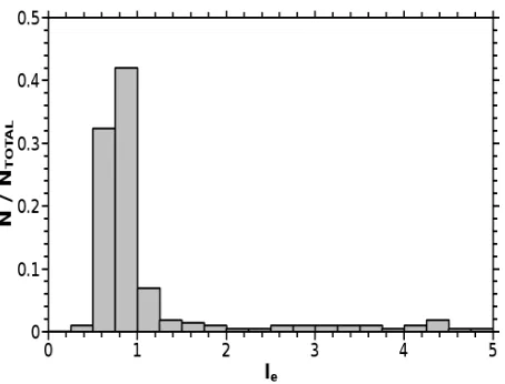
Figure 14. Ieis the number of iterations required for the number of objects

which have their estimate of luminosity class altered to drop by a factor of e, as determined by linear regression. Ieis a measure of the gradient of plots

like Fig. 13, where lower values of Iecorrespond to steeper gradients and

so quicker convergence.

4.4 Coping with unresolved substructure & photometric

errors

InMEAD, once estimates of distance and extinction are produced for each object, the data are binned, with respect to distance, to pro-duce a distance-extinction relationship. As discussed in Section 3, the extinction will not be uniform for a finite sized box at any given distance. Instead it will vary with sky angle, just as it will vary with depth, due to unresolved substructure prompting some intrin-sic variation in extinction. Hence, in this study, the extinction in any given bin is characterised as having some intrinsic scatter.

If the photometric errors are propagated through to give the error on the determined value of the extinction, it is possible to determine Maximum Likelihood Estimators (MLEs) for the mean and intrinsic standard deviation of the extinction, if the character of the variation in extinction is known. If the variation of extinction is

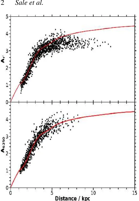
Figure 15. The difference between the values of mean monochromatic ex-tinction at 6250 ˚A at a given distance determined byMEAD(Aout) and the

value in the simulation (Ain). The simulation has had intrinsic scatter in

ex-tinction imposed in a manner consistent with Kolmogorov turbulence in the ISM.

Gaussian, then the estimate of the mean value of the extinction in each bin ( ¯A) is given by the following equation:

¯ A=

∑

i Ai

σ2 ¯

A+δA

2

i

∑

i

1

σ2 ¯

A+δA2i

, (5)

where Aiis the estimated extinction for a single object, and other

terms are as described in Section 4.3:

This estimate is essentially a weighted mean of the individual estimates of extinctions for each object in the bin. It is found that the intrinsic scatter of extinction in each bin (σ_A¯) can be

satisfacto-rily estimated by the weighted standard deviation of the extinctions of the brighter objects in the bin (those with dA625060.1). The

weighting for this estimate is the weight given by equation 3 over dA2

6250.

In reality, the intrinsic scatter of extinction in each distance bin is a result of the turbulent processes at work in the ISM. If the extinction of each simulated object is scattered away from the mean value for the distance as a result of Kolmogorov turbulence,MEAD

still successfully retrieves the input extinction, despite the in-built assumption that extinction at a given distance is scattered normally (Fig. 15).

4.5 Handling of magnitude limits

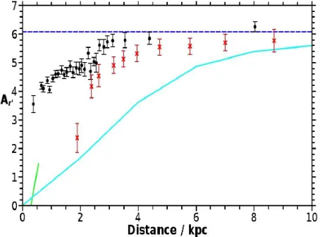
out-Figure 16. Setting the value of n too low in equations 1 and 2, thus compromising the results ofMEAD. Here the upper panel shows n=0.5 and the lower n=2.0. Both panels are for 50 iterations in the direction

(l,b) = (180,0), the actual (input) distance-extinction relation is the red line and the black points are the results fromMEAD.

Figure 17. The variation in the total number of data points (black dots, left axis) and proportion of bad data points (red crosses with error bars, right axis) on the derived distance-extinction relation as a function of n for the directions(l,b) = (80,0),(130,0),(180,0). Where good bins are those which satisfy the condition Aout−Ain<σ2A+δ2A¯ and bad bins are those

which do not.

come. Although many of the objects filtered out should be removed for reasons of incompleteness, others need not be and are lost un-deservedly. A compromise is necessary. We set n=2 so as to use the maximum possible number of objects whilst avoiding the mag-nitude limit effect. Fig. 17 illustrates that setting n=2 obtains the highest number of accurate distance bins on the derived distance-extinction relationship whilst maintaining a low proportion of bad bins.

4.6 Achievable angular resolution

Previous observational 3D extinction maps of the Milky Way (Fitzgerald 1968; Lucke 1978; Neckel et al. 1980; Pandey & Mahra 1987; Joshi 2005, e.g.) have been carried out at angular resolutions of the order of a few degrees. The recent extinction map due to Marshall et al. (2006) has a resolution of 30′. With the high angular density of sources in the IPHAS database (∼105sq.deg.−1_{) it is clearly possible to map extinction at a much}

finer angular resolution. The resolutions possible are dependent on the source density, but even in the relatively sparsely populated galactic anti-centre resolutions of 10′are achievable.

4.7 Bias in distance estimation

The estimate of the distance modulus to each object has a symmet-ric error distribution around its mean. However, the expected distri-bution of stars is not symmetric as the volume of space in which a star lies and the density of stars changes. Therefore, the expectation of the true distance to the star does not equal the original estimate and so that original estimate is biased. An analogous effect leads to the well known Lutz-Kelker bias (Lutz & Kelker 1973), when using trigonometric parallaxes to estimate the absolute magnitudes of objects. Following Lutz & Kelker (1973) it is possible to derive a correction for this bias, if the density of stars is assumed to be uniform. If this correction is applied to the distance bins of ob-jects from the simulated photometry, where the stellar density is assumed to be uniform, the median correction is found to be 0.1%, whilst 95% of bins have corrections less than 1%. The improvement on the agreement between the input and derived extinction-distance relationships is thus negligible.

Calculating a correction for a realistic density distribution is considerably more difficult. However, the median correction will often be smaller than in the case of uniform stellar density, because of the drop off in stellar density associated with most sightlines.

4.8 Sensitivity to disc metallicity gradients

The Besanc¸on model assumes a smooth gradient in the mean metallicity with respect to galactocentric radius (RG). This

view is shared by Friel et al. (2002) and Bragaglia & Tosi (2006) amongst others. However, it has been argued (e.g. Twarog, Ashman & Anthony-Twarog 1997; Corder & Twarog 2001; Yong, Carney & Teixera de Almeida 2005) that metallicity in fact varies as a step function of RG, with the step occurring

at RG∼10 kpc. Carraro et al. (2007) and Bragaglia et al. (2008)

argue that any gradient flattens to a constant metallicity in the outer disc. Given this spread in opinion it was necessary to test the performance ofMEADagainst a range of different schemes.

on the other hand, are metallicity dependent, but these do not be-come significant until metallicities are markedly sub-solar (Fig. 5). Consistent with this we find that introducing metallicity variations induces little change in the output fromMEAD, even thoughMEAD

assumes solar metallicity. This is true of all the above mentioned schemes for the disc metallicity gradient.

4.9 Correction for binarity

Unresolved binaries and higher multiples present the possibility of the systematic over-estimation of point-source absolute mag-nitudes. For the objects selected byMEAD(A0-K4), the effect of binarity on the observed colours is small (Hurley & Tout 1998).

In the extreme case of binaries of unit mass ratio the distance to an object would be underestimated by a factor of√2 compared to the single-star case. However, on making plausible allowances for the binary mass ratio distribution and for the binary fraction, it is likely that, in the mean, distances will only be underesti-mated by a factor of a few percent. For example, the expected un-derestimate of distance will be∼5% if the Kroupa (2001) IMF, Duquennoy & Mayor (1991) binary fraction, a constant probabil-ity function for binary mass ratio and a mass-luminosprobabil-ity relation of L∝M3.5are all assumed.

To arrive at a correction factor that may be applied routinely withinMEAD, the effect of binarity has been analysed through the use of simulated photometry. Binaries were inserted in the model using a binary fraction of 57%, following Duquennoy & Mayor (1991) which is derived from observations of G-type stars. Lada (2006) demonstrates that the binary fraction drops significantly for later type stars, but these are mostly those which are not simulated (i.e. M-type stars and later). The probability function for the binary mass ratio was assumed to be constant, whilst higher order unresolved multiples are assumed to be relatively rare (Duquennoy & Mayor 1991) and so are not included in the simula-tion.

The outcome of this exercise is that there is systematic un-derestimation of distances, which in turn causes extinction to be overestimated in a given distance bin. The appropriate correction for this is made by multiplying all the derived distances by 1.06. This figure was derived through minimisation of the statistic in equation 4, over 100 visualisations of 6 different sightlines. This modification should function successfully as most bins contain rel-atively large numbers of objects and the correction itself is small. When this correction is adoptedMEADsuccessfully reproduces the input distance-extinction relationship.

4.10 Impact of reddening law variations

MEADand the simulations performed up until this point assume the R=3.1 reddening law of Fitzpatrick (2004). To investigate the ef-fect of altering R significantly, simulated photometry was created with R=2.6 and 3.6 reddening laws. ThenMEADwas run on the results of these simulations, while continuing to apply the R=3.1 law. Fig. 18 shows that the impact onMEAD’s mapping of sightlines better represented by non-standard reddening laws is to induce a systematic error that is comparable - in these examples - with the typical random error. Had the reddening been expressed in terms of the monochromatic extinction, A6250, Fig. 18 would look much

the same. However, a conversion into AV, would be even more

de-pendent on the value of R and therefore the outcome of a mapping expressed in terms of AV would be subject to even greater

system-Figure 18. The effect of altering the value of R on the difference between the values of mean broadband extinction in the r′band at a given distance determined byMEAD(A(r′)out) and the value in the simulation (A(r′)in).

The results for R=3.6 are represented by unfilled black bars bounded by solid lines, R=2.6 by hatched red bars bounded by dashed lines. The sim-ulations are for the direction(l,b) = (180,0)and 50 visualisations were performed in each case.

atic error. The sense of the bias is that the extinction at a given distance for sightlines of anomalously high R is underestimated.

Given that IPHAS observations provide magnitudes in just three bands, it is not feasible to constrain R in addition to the in-trinsic colour, extinction and luminosity class (and so distance). Instead it is preferable to rely on the relative dominance of the R=3.1 reddening law across the Galactic Plane. The same assumption has been made previously by Neckel et al. (1980); Schlegel et al. (1998); Marshall et al. (2006) and many others. If the IPHAS database were to be cross-matched with the results of the United Kingdom Infrared Deep Sky Survey Galactic Plane Sur-vey (UKIDSS GPS; Lucas et al. 2008) and the Ultraviolet Excess Survey of the northern Galactic Plane (UVEX; Groot et al. in prepa-ration) the extra measurements would facilitate the accurate mation of R, whilst still maintaining the accuracy of the other esti-mates.

4.11 The impact of very young populations

O, B and very early A stars occupy the same area of the IPHAS colour-colour plane as less-extinguished later A and F stars. How-ever, they also respond differently to extinction and have different absolute magnitudes and so introduce a degeneracy into the prob-lem. In the inter-arm field such objects are comparatively rare, with their short lifespans and the IMF suppressing their frequency. How-ever, in the spiral arms such objects are more frequent, due to the on-going star formation induced by the passage of the spiral density wave. The Besanc¸on model makes no allowance for spiral-arm in-duced star formation, since a constant star formation rate is adopted for all locations. Therefore simulations based on the Galactic model cannot provide any insight into the impact of these localised young populations. We have carried out some tests of such concentrations by inserting them into model sightlines in order to mimic the super-position of a spiral arm. The results show no additional systematic error in the derived extinction curves that would imply a breakdown of the method.

in-troduce degeneracy, due to their different colours, absolute mag-nitudes and response to extinction as compared to the sequences assumed in the calibration ofMEAD. Also, as with early-type stars, PMS objects would normally be found concentrated in star forming regions. So as to investigate the effect of including PMS objects the extra spiral arm population was again included in the model. The inserted PMS objects were then tracked throughMEAD. In reality, many PMS objects exhibit Hαemission and so lie outside the main stellar locus on colour-colour plots and are thus ignored byMEAD. However, those PMS objects exhibiting weaker Hαemission would remain inside the main stellar locus, where they may be misiden-tified by MEAD. As with O and B stars, the relative scarcity of emission-line PMS stars compared to normal stars should limit this problem. As a direct test of this and other expectations regarding young populations, we present and discuss the example of sight-lines through Cyg OB2, a spectacular northern OB association, in section 5.3.

4.12 The impact of photometric zero-point errors

At the time of writing the IPHAS database lacks a global calibra-tion, with observations instead being calibrated on a run by run basis, with the Hαcalibration tied to the r′calibration. As such it is possible that there will be offsets between the true and mea-sured magnitudes in one or more bands. To investigate the effects of such difficulties, offsets were manually introduced into the sim-ulated photometry.

The effect of adding the same magnitude offset to all three bands is simple to understand, as this will simply lead to inaccurate determinations of the distance to each object. For example an offset of 0.10 mags is well within the range of what might be encountered within the IPHAS database presently. This offset leads to a 5% error in determined distances.

Somewhat less straightforward is the effect of offsetting one band only, as this will affect the intrinsic colours and extinctions de-termined for each object, and so the object distance as well. Fig. 19 shows the effect of applying a positive and negative offset to Hα. There are two consequences of doing this. The first is that the ac-curacy ofMEADis reduced, as all objects are now systematically misidentified. This effect can be seen clearly by comparing the two panels in Fig. 19. Second,MEADreturns fewer points, for the case of a negative offset to Hα. This can be very serious as it may re-duce the number of returned points significantly. In the case shown 90% of the objects available are lost: this is because the main stel-lar locus has shifted stel-largely outside the region of the colour-colour diagram searched byMEAD.

Until a global photometric calibration is performed, tying the Hαcalibration to r′vastly reduces the frequency and size of offsets in the (r′−Hα). In the future the calibration in the i′band will also be tied to the r′band calibration, improving the suitability of the data for use inMEAD.

5 EXAMPLE APPLICATIONS OF MEAD

5.1 A sightline in Aquila, through (l,b=32.0,2.0)

For this direction, the results from this work (Fig. 20) show two significant increases of extinction, one within the first few hundred parsecs, which would be associated with the Aquila Rift. The Rift is at a distance of∼200 pc (Dame et al. 1987), with the extinction ris-ing to AV≃3 (Ar′≃2.5) (Straiˇzys, ˇCernis & Bartaˇsi¯ut˙e 2003). We

Figure 19. The top panel shows the retrieved extinction-distance relation-ship, given an offset of 0.05 (black dots) or−0.05 (green crosses) to the Hαmagnitudes of the objects. The bottom panel shows the results with no offset (black dots). On both panels the input relationship is shown as the red line. The simulations are for the direction(l,b) = (180,0).

Figure 20. Distance-extinction relationship for field 4199 in the direction