Tracking of moving objects using mathematical imaging

1

Faculty of Electrical Engineering,

Mathematics & Computer Science

Tracking of moving objects

using mathematical imaging

Jesse Zwienenberg B.Sc. Thesis

July 2017

Supervisor:

Abstract

Estimating the motion of objects in image sequences is a problem which arises in several research areas like image processing, bio-medical imaging and machine vi-sion. The motion induced on the image plane by the objects is called the optical flow and in this work we compute this using two vastly different methods. Firstly we look at variational models which use the image derivatives in the setting of convex energy functional minimization to compute the optical flow between images. The second method that we discuss is known as deep learning and revolves around the usage of convolutional neural networks. To compare the performance of both meth-ods we implemented the variational models from scratch and for the deep learning approach we use a publicly available pre-trained model.

Contents

Abstract iii

1 Introduction 1

1.1 Overview . . . 1

1.2 Outline . . . 2

2 Optical Flow 3 2.1 Optical flow constraint . . . 3

2.2 Difficulties . . . 5

2.3 Representing flow fields . . . 6

2.4 Benchmarks . . . 7

3 Variational Methods 9 3.1 Variational models . . . 9

3.1.1 Data terms . . . 10

3.1.2 Regularization terms . . . 11

3.2 Numerical realization . . . 13

3.2.1 Implementation . . . 14

4 Deep Learning 19 4.1 How deep learning works . . . 19

4.1.1 Activation functions . . . 20

4.1.2 Learning . . . 20

4.1.3 Convolutional neural networks . . . 22

4.2 FlowNet 2.0 . . . 23

5 Testing 25 5.1 Error measures . . . 25

5.2 Variational Methods . . . 26

5.2.1 The effect of alpha . . . 26

5.3 Deep Learning . . . 27

5.3.1 Components . . . 27

VI CONTENTS

5.3.2 Performance . . . 28

5.3.3 Robustness against noise . . . 29

5.4 Comparison . . . 31

5.4.1 Performance . . . 31

5.4.2 Robustness against noise . . . 33

6 Conclusions and recommendations 35 6.1 Conclusions . . . 35

6.2 Recommendations . . . 35

Chapter 1

Introduction

1.1 Overview

The analysis of image motion plays a big role in computer vision. This is a field which aims to give computers the ability to understand images and videos on a high level. Application wise there is a very wide range of areas in which the analysis and estimation of image motion is useful. These applications range from recognizing human activity in the recordings of video surveillance systems to tracking biological cells in microscopic videos. Other notable examples of applications are motion com-pensation for video compression and estimating the 3D scene layout from 2D video footage.

In this paper we are specifically interested in determining the underlying 2D mo-tion of objects in image sequences. This is what is called the optical flow. So given any two consecutive frames in a sequence of images we are looking to create a field of vectors such that every vector represents how the object at that specific position is moving in between the two frames. This is called a flow field and an example of what this looks like, is shown in Fig. 1.3. This field represents the optical flow between two images from the ’Hamburg Taxi’ sequence [1].

Figure 1.1: Image 1 [1] Figure 1.2: Image 2 [1] Figure 1.3: Flow field

2 CHAPTER1. INTRODUCTION

The first method for computing the optical flow that we look at is the variational method. This method follows from the mathematical formulation of basic assump-tions about image motion. We solve the minimization problem that follows from these assumptions using a primal-dual algorithm.

The second method is the deep learning method, which uses very large con-volutional neural networks. These networks extract abstract image-features and compute the optical flow based on these features. The models are trained on data of which the underlying motion is known. Through this training the models learn how they should extract and combine the image-features to accurately compute the optical flow.

Variational methods are driven by theory and have been around in image analy-sis for a long time. On the other hand deep learning methods are data-driven and only recently gained popularity. Since there is such a big difference between the ap-proaches of both methods it is interesting to see how their performances compare with each other.

1.2 Outline

In this work we review two different approaches to optical flow computation. We start by taking a closer look at the optical flow and describing it in a mathematical way in Chapter 2. We describe problems that come up which make computing the optical flow a difficult task.

Then in Chapter 3 we discuss variational methods for optical flow computation, the first of the two approaches that we discuss. After introducing the general concept of variational methods we explore and compare different possibilities inside this frame-work. After this we look at a numerical implementation of these methods.

In Chapter 4 we look at a totally different approach known as deep learning. We show what convolutional neural networks look like and how they can be used to compute the optical flow.

In Chapter 5 we put the discussed methods in practice. We show how they perform on several datasets and compare aspects of their performance.

Chapter 2

Optical Flow

Finding the optical flow comes down to recognizing corresponding objects between two images. So for any objectXfrom the first image we are given the task of finding an object Y in the second image which corresponds to object X. If we are able to find such an object Y, we can estimate the optical flow with the vector between the position of X and the position of Y (scaled according to the time between the images). For this task of finding corresponding objects we can use the assumption that if we make sure the time between two images is small enough, the object will look the same in both images, the only difference being that it might be slightly translated across the axes of the image. There are several obvious cases in which this assumption fails, examples are objects which become occluded or inconstant lighting casting shadows on the scene which change the appearance of moving objects over time. These things are points of attention, but in most cases the majority of objects in a scene will look approximately the same in consecutive images, so this assumption is a reasonable starting point.

2.1 Optical flow constraint

Let us introduce some notation to turn this assumption into an equation. Let x = (x1, x2)| ∈R2 denote a spatial position andt∈[0, T]a certain point in time. Now let

u(x, t)be a representation of the appearance of the pixel at positionxon the image taken at time t. This representation can have multiple dimensions, for example the RGB-values of the pixel. In this work however we use u(x, t) to denote the

brightness, the simplest representation of the pixel.

4 CHAPTER 2. OPTICALFLOW

Consider an object X which is located at position x on the image taken at time t. Let’s denote the displacement of X between this image and the next one by the vector ∆x and the time between the images by the scalar ∆t. We expect the

brightness of object X to be the same in both images so now we can formulate the followingbrightness constancy constraint:

u(x, t) =u(x+ ∆x, t+ ∆t). (2.1)

We can rewrite the right-hand side as a Taylor Series at the point(x, t) and under

the condition that both ∆x and ∆t are small we can can ignore the higher order terms.

u(x+ ∆x, t+ ∆t)≈u(x, t) + ∂u

∂x1

∆x1+

∂u ∂x2

∆x2+

∂u ∂t∆t.

When it comes to determining optical flow the displacement∆xis unknown and the displacement per time unit ∆x

∆t is what we actually want to compute. So the next

step is canceling out the common term u(x, t)and dividing everything by∆t, which yields:

0 = ∂u

∂x1

∆x1

∆t + ∂u ∂x2

∆x2

∆t + ∂u ∂t .

In the literature this is often written in a slightly cleaner way by using ut to denote ∂u

∂t and ∇u to denote the gradient of the image data, a vector containing the two

spatial derivatives of the image,∂u ∂x1,

∂u ∂x2

|

. Also v = (vx, vy)|is used to denote the

estimation of the optical flow ∆x

∆t =

∆x1

∆t ,

∆x2

∆t

|

, yielding:

∇u·v +ut = 0. (2.2)

This equation is generally known as theoptical flow constraint. It is used in the

2.2. DIFFICULTIES 5

2.2 Difficulties

The optical flow constraint exposes some inherent problems of motion perception. The constraint forms a linear system with n linear equations, where n is the num-ber of dimensions of u(x, t). This system has a unique solution if there are two

independent equations since there are two unknowns, vx and vy. The brightness is

one-dimensional so in our case the system consists of only a single equation, hence this system does not yield a unique solution. Only the component in the direction of the image derivatives (ux, uy)| can be determined. We can not say anything about

the component in the direction perpendicular to these derivatives, based on this system. Furthermore when all image derivatives are zero the optical flow constraint gives us no information about the motion at all. This occurs in the interior of uniform regions, where anyv would satisfy the optical flow constraint.

This problem of an underdetermined system as a result of the optical flow constraint is known as the aperture problem. This problem tells us that certain combinations of motions of objects can cause identical looking images. As a consequence there will be cases in which there is no way to uniquely determine the underlying motion based on the image data alone. This means that if we want to use the optical flow constraint to compute the optical flow at locations like this we need extra constraints to obtain unique solutions.

In the previous section we mentioned a couple of occasions where the constancy assumption (equation 2.1) is not fulfilled at all. Apart from these situations we need to take into account that image data is not perfect and consequently the brightness constancy constraint will not hold perfectly most of the time. First of all the data is a discretization of the reality, this can cause objects to be displayed slightly different between images especially when the resolutions of the images are low. Secondly, noise in the data can cause disturbances in the fulfillment of the optical flow con-straint.

6 CHAPTER 2. OPTICALFLOW

For an in-depth analysis of other basic problems and concepts related to optical flow estimation we refer to [2].

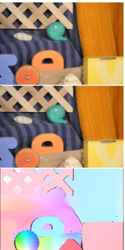
2.3 Representing flow fields

Representing the flow field with arrows is difficult to interpret in some cases, so often the motion is indicated by a color coding instead. In Fig. 2.4 we see how the flow field from Fig. 2.3 can be represented using colors. The color indicates the direction of the vector and the intensity goes up as the absolute value of the vector gets larger, which indicates a higher velocity. This is visualized by the colorwheel in Fig. 2.5.

Figure 2.1: Image 1 [1] Figure 2.2: Image 2 [1]

Figure 2.3: Arrows Figure 2.4: Color-coding

2.3. REPRESENTING FLOW FIELDS 7

2.4 Benchmarks

The Middlebury database [5] is often used as a bench-mark to assess the relative performances of optical flow algorithms. It is a small dataset of image sequences of which the ground-truth flow is determined through dif-ferent measurements. This dataset addresses difdif-ferent challenging aspects of flow estimation and it introduced an online evaluation and ranking for optical flow algo-rithms.

Some more image sequences and their ground-truth flows are presented by the KITTI database [6]. This data base includes the frames of videos recorded by the cam-era on top of a driving car. The ground truth flow is deter-mined using a laserscanner which is also located on top of the car. This dataset contains realistic data of outdoor scenes, however the ground-truth flow is sparse since the movement of the sky can not be captured using the laser scanner.

Another commonly used benchmark is the MPI Sintel dataset [7]. This dataset consist of rendered scenes of an animated movie. Since the scenes are artificial the ground-truth can be easily determined. This dataset is the largest of the three and contains over a thousand im-age pairs.

Examples of image pairs and their ground-truths from each of these datasets are displayed in Fig. 2.6, 2.7 and 2.8.

Figure 2.6: Middlebury

Figure 2.7: KITTI

Chapter 3

Variational Methods

The first implementation of a variational method for optical flow computation was the Horn-Schunk method [8] constructed by Horn and Schunk in 1981. Since then better and more complex methods have been developed (e.g. [3]), but the essence of variational methods has remained the same. As mentioned earlier most variational methods for optical flow estimation use the optical flow constraint as a foundation. The main problem of this constraint is its possible ambiguity due to the aperture problem. To overcome this problem and to get to a unique result, an additional constraint is added. This constraint should impose some kind of structure on the solution that we would expect actual flow fields to have.

The additional constraint that the Horn-Schunk method used was based on the assumption that flow fields vary smoothly almost everywhere. For the interior areas of objects this assumption makes a lot of sense, in these areas we can expect neighboring points to have similar velocities. However, for points on the edges of objects it is different. At the edges of objects neighboring points can belong to entirely different objects which can have entirely different velocities so discontinuities can be expected. This means that methods using a smoothness constraint are likely to have difficulties determining the correct flow around the edges of objects.

3.1 Variational models

The basic idea of variational models for optical flow computation is to use a sec-ondary constraint alongside with the optical flow constraint to find a solution which agrees with both of them as well as possible. This is done through the usage of energy functionals. For a given image sequenceuwe want to assign a certain mea-sure of ’energy’ to any possible flow fieldv, this energy serves to indicate how well both constraints are met. When the constraints are fulfilled this energy gets very small and violations of the constraints lead to higher energies. Through minimizing

10 CHAPTER 3. VARIATIONALMETHODS

this energy we wish to find avwith a very low energy, indicating it fits our constraints well. In general these variational models are of the form:

min

v D(u, v) +αR(v). (3.1)

Here,D(u, v)is called thedata term, it takes as input the image datauand a possible solution v. To make sure the optimal solution vˆ of the expression (3.1) does not

violate the optical flow constraint too much, this function is defined in such a way that the output gets bigger asv obeys the optical flow constraint less strictly.

The other termR(v), called theregularization term, does not use the image data.

The purpose of this term is basically to measure how likely it is for any particular v to be an actual flow field, regardless of the image sequence. As mentioned before a way of doing this is by looking at the smoothness of the field v. In general this is what most regularization terms do, they get very small whenv is smooth and larger when the smoothness constraint is violated.

Theαis a scalar deciding the relative importance between the two terms. Choos-ing the appropriate α comes down to deciding how well we expect the actual flow field to agree with the optical flow constraint. For noisy images we need to set α to a higher value. Due to the noise, the actual flow field violates the optical flow constraint by some amount, so we really need the regularization term to enforce smoothness even if that means the optical flow constraint gets violated more. For ’cleaner’ images we do not really need the regularization term to force the smooth-ness as much. In this case its task is better described as picking the most smooth field out of the possible solutions v that agree with the optical flow constraint really well. For this task it is better to setαto a lower value.

3.1.1 Data terms

We mentioned that we want the data term to give a certain ’punishment’ to possible solutions v for violating the optical flow constraint. We define such a function by calculating how much it violates the optical flow constraint for every position x and then take a norm. Conventional choices for this norm are either the L1 _{norm or the}

squaredL2 _{norm, yielding:}

DL1(u, v) := k∇u·v +utk₁ and

DL2(u, v) :=

1

2k∇u·v+utk

2 2 .

3.1. VARIATIONAL MODELS 11

of this squared L2 norm is that outliers do have a huge impact on its value, so this

method does not allow the solution to violate the optical flow constraint by a very large amount. This is not always preferable. In this respect the L1 norm handles

outliers in a more robust way. Here, outliers in the data are less destructive to the solution.

3.1.2 Regularization terms

The regularization terms that we mention here serve to give some measure of smoothness to the flow fields. This can be done by looking at the gradient of the flow field∇v, which you want to be close to0most of the time if you expect the flow

field to be smooth. Two standard choices for the regularization term are:

RT V(v) :=k∇vk₁ and

RL2(v) :=

1 2k∇vk

2 2 .

The Horn-Schunk method [8] uses the last option of the two, here the L2 _norm

is used to punish possible solutions v for having a gradient which is not close to

0 at several positions. Just like with the L2 _{data term, the L}2 _{regularization term}

is punishing outliers really heavily. This will generally lead to solutions which do not have any of these outliers, meaning it is likely to be a completely smooth field. Again, this might not always be what we want, flow fields need not to be smooth everywhere. In fact most of the time we want the field to have sharp edges instead of smooth transitions at the very edge of the objects. The total variation (T V) of v is a regularization term which generally allows these sharp edges to exist, since the punishment for outliers is not as extreme in this case. Also where the L2 _{term has}

very low punishment for small deviations from0, theT V term enforces this constraint linearly. So when minimizing theT V term, there is still a relatively big incentive to push small deviations from0 even closer to0. This will generally result in solutions

which are approximately constant everywhere except at the edges of objects where sharp edges occur.

Extended regularization terms

We can choose between RL2 and RT V to either create a smooth solution or a

12 CHAPTER 3. VARIATIONALMETHODS

extension of the following form is proposed:

R(v) = inf

w α0

2

X

i=1

k∇vi−wk₁+α1S(w). (3.2)

Here, a new variablewis introduced to shift the derivatives ofv, and a functionS(w)

which forces thiswto be small. The usage of theL1norm ink∇vi−wk1is supposed

to create the sharp edges and we need wto facilitate the general smoothness ofv. Also instead of a single value for α we will have two parameters. Here α0 has a

role similar to that ofαin the standard regularization terms, it determines the weight of the smoothness constraint relative to the optical flow constraint. Now α1 can be

chosen in proportion to α0. When α_α0₁ is chosen to be large this indicates that the

piece-wise constant parts outweigh the smooth parts and the opposite when α0

α1 is

small.

We can achieve the smoothness in the solution by using the squared L2 norm

of was S(w). Doing this makes sure wwill be small and does not contain outliers, which enforces a certain smoothness on w. We expect ∇vi −w to be piece-wise

constant, since we use theL1 norm. If we then add the small smooth field_wwe can

expect∇v to be piece-wise smooth, which is what we wanted.

Another way of achieving smoothness is by minimizing higher order derivatives ofv. If we defineS(w)to be theL1 norm of_∇wwe achieve something similar to this

since the first part of the extended regularization term leads towbeing close to∇v.

Effectively we are minimizing something which is close to∇2v. By letting this part of

the regularization term work alongside the first part we want to generate solutions which are smooth and contain sharp edges

This gives us the following definitions for the extended regularization terms:

RT V /L2(v) := inf

w α0

2

X

i=1

k∇vi−wk₁+

α1

2 kwk

2

2 and

RT V /T V(v) := inf w α0

2

X

i=1

3.2. NUMERICAL REALIZATION 13

3.2 Numerical realization

The optical flow constraint at a certain pixel is only dependent on the solution v at that pixel. However, this is not the case for the regularization terms. Changes at a certain position in v will cause changes in ∇v in an area around this position. This means we can not divide the problem into independent parts and to solve the minimization problem we need an efficient method which solves problems of the form:

min

v D(u, v) +αR(v).

A commonly used method for solving minimization problems is gradient descent. This method uses the partial derivatives of the objective function to determine where the minimum is located. This minimum is iteratively approached by taking steps in the direction of the negative of the gradient. One of the requirements of this methods is that the objective function needs to be differentiable. The regularization terms that we mentioned are non-smooth and hence not differentiable. For this reason basic minimization schemes like gradient descent do not work.

A minimization scheme that does work for this problem is the first-order primal dual algorithm described in [9]. This algorithm converges to a solution at the rateO(1/N)

and applies to problems of the form:

min

x F(Kx) +G(x). (3.3)

WhereF and G are proper, convex1, lower semi-continuous2 functions and K is a continuous, linear operator.

The algorithm acts on a so-called primal-dual problem which follows from the primal problem (3.3). This primal-dual problem is of the form:

min

x maxy hKx, yi+G(v)−F

∗

(y). (3.4)

The algorithm iteratively approaches the solution x,ˆ yˆ of the primal-dual problem

(3.4). In every iteration the value x and y are approximated as a function of the x andy of the previous iteration. How this iterative scheme is defined can be seen in Fig. 3.1.

1_{f(θx+ (1−θ)y)≤θf(x) + (1−θ)f(y) ∀θ∈[0,1]} 2_{lim inf}

x→x0

14 CHAPTER 3. VARIATIONALMETHODS

Primal-dual algorithm [9]

Choose: τ, σ >0, θ∈[0,1], (x0_{, y}0_{)∈X×Y, x¯}0 _=x0

yn+1 = (I+σ∂F∗)−1(yn+σKx¯n)

xn+1 = (I+τ ∂G)−1 xn−τ K∗yn+1

¯

xn+1 = xn+1+θ xn+1−xn

Where:

(I+τ ∂F)−1(y) = arg min

x

(

kx−yk2

2τ +F(x)

)

Figure 3.1:Scheme showing how variables are updated in the algorithm [9]

Here,F∗ is used to denote the convex conjugate ofF. The parts which are essential for the efficiency of this algorithm are the operators (I+τ ∂F∗)−1 and (I+σ∂G)−1

which are called the proximal operators. The algorithm will be efficient when these can be solved efficiently.

3.2.1 Implementation

To implement the models discussed in section 3.1 we need to convert the data- and regularization terms to functions F and G, determine suitable operatorsK and K∗ and find a way to compute the proximal operators. To make sure that the algorithm is efficient we need to formulate our problem (3.1) in such a way that the proximal operators can be solved efficiently. The proximal operators for the data terms can be solved efficiently as a function ofv, so we can useDas our functionG. However

3.2. NUMERICAL REALIZATION 15

can be used to make the algorithm work.

Implementation of the data terms

For the data terms we do not need the linear operatorK so they can be transformed toGstraight up. The data term DL1 leads to:

G(v) = kv· ∇u+utk1

and the termDL2 yields:

G(v) = 1

2kv· ∇u+utk

2 2 .

In case we use the regularization termRT V /L2 we will change this functionGslightly.

Implementation of the regularization terms

For the regularization terms we will need the operator K to act on v and possibly onw. For both the standard terms RT V and RL2 we can define K = ∇ as a linear

operator andK∗ =−∇·as its adjoint operator. ForRT V we get:

F(Kv) = αkKvk₁ =αk∇vk₁

and forRL2 we get:

F(Kv) = α 2kKvk

2 2 =

α

2 k∇vk

2 2 .

For the extended regularization terms the variable w comes into play. Our primal variable will change from v to (v, w). In the case of RT V /L2 we want our F to be a

function of∇v −w, so we get: K =h∇ −I

i

andK∗ =h−∇· −I

i|

. NowF can be defined as:

F (K(v, w)) =α0kK(v, w)k1 =α0k∇v−wk1 .

We want to add the last part of this regularization term RT V /L2 to the functionG so

depending on the data term this becomes:

G(v, w) = kv· ∇u+utk1+

α1

2 kwk

2 2 or

G(v, w) = 1

2kv· ∇u+utk

2 2+

α1

2 kwk

2 2 .

For the extended regularization term RT V /T V we do not need to make changes

to the original functionGand we wantF to be a function of(∇v−w,∇w)which we

get using the following operator and its adjoint:

K = "

∇ −I

0 ∇

#

, K∗ = "

−∇· 0

−I −∇·

#

.

NowF can be defined as:

16 CHAPTER 3. VARIATIONALMETHODS

Calculating the proximal operators

We are left with the task of computing the proximal operators. For any combination of the terms that we discussed, these will be efficiently solvable, there is even a closed form representation for all of them.

For the functionGwe have the following possibilities:

G(v) =kv· ∇u+utk₁

G(v) = 1

2kv· ∇u+utk

2 2

G(v, w) =kv· ∇u+utk1+

α1

2 kwk

2 2

G(v, w) = 1

2kv· ∇u+utk

2 2+

α1

2 kwk

2 2 .

The first option which comes from the usage ofDL1 leads to:

v = (I +σ∂G)−1(˜v) = ˜v+         

−τ∇u ifρ(˜v) <−τ(∇u)2

τ∇u ifρ(˜v) > τ(∇u)2

ρ(˜v)

∇u if |ρ(˜v)| ≤τ(∇u)

2

(3.5)

where ρ(v) =∇u·v+ut.

The second option for G comes from the usage of DL2 and leads to a proximal

operator which is representable as:

v = (I+σ∂G)−1(˜v) =

a3b1−a2b2

a1a3−a22

,a1b2−a2b1 a1a3−a22

(3.6)

for:

a1 = 1 +τ uxux b1 = ˜v1−τ uxut

a2 =τ uxuy b2 = ˜v2−τ uyut

a3 = 1 +τ uyuy .

For the last two instances ofGwhere the variablewplays a role due to the usage of the regularization termRT V /L2 we will get a solution of the form (v, w)wherewcan

be computed seperately. We can calculatev in the same way as we just did in (3.5) and (3.6), where there was now.

(I +σ∂G)−1(˜v,w˜) = (v, w)

where

w= w˜ 1 +τ α1

3.2. NUMERICAL REALIZATION 17

For the functionF we have the following possibilities:

F (Kv) = αkKvk₁

F (Kv) = α 2 kKvk

2 2

F (K(v, w)) = α0kK(v, w)k₁

F (K(v, w)) = α0k∇v−wk₁+α1k∇wk₁ .

For the last instance we can calculate its solution (I+τ ∂F∗)−1(˜p,q˜) = (p, q)

sep-arately for p and q as functions of respectively p˜ and q˜where (˜p,q˜) = K(v, w) = (∇v −w,∇w). So all we need to do is to find the proximal operators of the convex

conjugate of the following functions:

F(p) = αkpk₁ and

F(p) = αkpk2₂ .

In case we choose the regularization term RT V or RT V /L2 we want to compute

the proximal operator using the convex conjugate of F(p) = αkpk₁ and for RT V /T V

we want to do this twice, forpand forq. First we determine the convex conjugateF∗ which is:

F∗(p) =αδB(L∞₎

p

α

where δB(L∞₎

p

α

:=

  

0 forkpk∞ ≤1

∞ otherwise .

Using this, the proximal operator can be determined which results in:

p= (I+τ ∂F∗)−1(˜p) = min (α,max (−α,p˜)) . (3.8)

For the regularization term RL2 we want to compute the convex conjugate of

F(p) = αkpk2₂ which is:

F∗(p) = 1 2αkpk

2 2 .

Using this leads to the following proximal operator:

p= (I+τ ∂F∗)−1(˜p) = α

α+σp˜. (3.9)

Chapter 4

Deep Learning

Recently deep learning methods have become popular in several fields, including computer vision. An example of an interesting application is described in [11]. Orig-inally these methods were only used for tasks like classification which is vastly dif-ferent from computing the optical flow in the sense that the latter requires a per-pixel solution. With recent progress in areas which do require per-pixel solutions like se-mantic segmentation and depth estimation it has become increasingly interesting to approach the optical flow problem using deep learning methods.

4.1 How deep learning works

A deep learning model is in essence a function with a very large amount of pa-rameters, which predicts the ’label’ of the input. What this label is depends on the application, in our case it would be the optical flow of the input images. A general deep learning model could be described as:

ˆ

y=f(x;θ).

Here yˆ is the prediction of the label of input x using parameters θ. This function f is described by a large artificial neural network which consists of many neurons in a layered structure. You typically have an input layer which receives the input x= x0 and givesx1 as output using the parameters θ1. This output is then used as

input for the next layer. The layers after the input layer, the so-called hidden layers, sequentially determinex2, x3,· · · according to their parameters:

xi =fi(xi−1 ;θi).

Finally the last layer, the output layer, takes the output of the last hidden layer and determines the predictionyˆ..

ˆ

y=fn(xn−1 ;θn) =fn(fn−1(xn−2 ;θn−1) ;θn) = · · · .

20 CHAPTER4. DEEPLEARNING

The layers consist of a certain amount of neurons and some ’activation functions’. Every neuron in layer i has connections to neurons from the previous layer i−1

through which it receives its inputsxi−1. Each connection has a certain weight, the

weights of all the neurons in a single layer form θi. The neuron uses these weights

to take a weighted sum of its inputs and pass it through the activation function. The outputs of all these neurons form xi, which is given as input to the next layer.

The purpose of the neural network is to grasp certain abstract features of the input and make a prediction for the solution based on these features. The depth cre-ated through the use of multiple layers enables the network to model more complex behavior.

4.1.1 Activation functions

If we were to choose linear activation functions we would just get a linear transfor-mation of the input at every layer. This would defeat the whole purpose of having many layers since it would result in an output which is just a linear combination of the inputs. We want the network to be able to catch more interesting non-linear behav-ior so that is why it is important to choose nonlinear activation functions. Common choices are either the sigmoid function:

φ(x) = 1

1 +e−x , (4.1)

or a rectified linear unit(ReLU):

φ(x) =   

x x >0

0 otherwise . (4.2)

4.1.2 Learning

The architecture of the neural network facilitates the extraction of features but de-ciding which features are important to the solution and how these features should be extracted is something which is done by the weights of the connections. We could try to set these parameters manually, but except for the fact that the amount of weights gets enormous we also do not know how abstract features contribute to our solution most of the time. Instead of manually doing this, the parameters will be decided through supervised learning. This means that we use data of which we know the correct solution to train the network so it learns how it can make accurate predictions. So given data x1, x2,· · · of which we know the correct labels y1, y2,· · ·

we want to change the parameters θin such a way that for alli:

4.1. HOW DEEP LEARNING WORKS 21

To achieve this, the parameters will be adjusted through a process which is known as backpropagation. Backpropagation uses a stochastic variant of the gradient descent method to determine how it should adjust the parameters that it wants to train. The objective function which we want to minimize will be some measure of how well the network is predicting the solution:

L(θ) =X

i

`(yi,yˆi) =

X

i

`(yi, f(xi ;θ)) .

Here the loss function` determines how good the prediction yˆi is. A typical choice

for this function`is the Euclidean loss:

`(yi,yˆi) =kyi−yˆik2₂ .

To minimize L(θ) we iteratively adjust θ and move it in the direction of steepest descent:

θi+1 =θi−λ∇θL(x;θ)

Here λ denotes the stepsize, which is called the learning rate in this context. To compute the direction of steepest descent −∇θL(x ;θ) we need to calculate the

partial derivatives of the objective functionL with respect to the parametersθ. The last layer directly influences the output of the network so the partial derivatives with respect to the parameters of this layer can easily be calculated as:

dL dθn

= dL

dyˆ

dyˆ

dθn

.

Given that the activation functions are differentiable we can now calculate the partial derivatives in the previous layer using the chain rule for differentiation:

dL dθn−1

= dL

dyˆ

dyˆ

dxn−1

dxn−1

dθn−1

,

dL dθn−2

= dL

dyˆ

dyˆ

dxn−1

dxn−1

dxn−2

dxn−2

dθn−2

,

· · · .

This can be extended all the way to the beginning of the network. For the partial derivatives with respect to weights in the start of the network we get a really long chain of partial derivatives. The derivative of the sigmoid function has at most an absolute value of 0.25, so if we would use the sigmoid function (4.1) as activation

22 CHAPTER4. DEEPLEARNING

a derivative of 1 for positive inputs preventing the gradient from vanishing, for this

reason variants of ReLU are used more often recently.

The stochastic variant of the gradient descent method differs from regular gra-dient descent in that it approximates the gragra-dient using only a small and randomly chosen batchB of the training data at each iteration:

∇θL(x;θ)≈ ∇θLB(x;θ)

where

LB(θ) =

X

i∈B

`(yi, f(xi ;θ)) .

This stochastic variant has two major upsides. Firstly this makes computing the gradient much less time consuming, especially since networks are generally trained on extremely large data sets. Secondly it adds a certain amount of randomness to the updates of the weights, which serves to avoid situations where the network gets stuck at a local minimum.

One problem which naturally comes up when systems with a large amount of parameters are optimized, is overfitting. This occurs when the system represents meaningless properties which are very specific to the training data instead of rep-resenting general features which still make sense for data outside the training set. This is also a serious problem in deep learning, but this can be easily solved by the dropout technique described in [15]. During training several neurons get ignored randomly to prevent the system from getting too reliant on a very small set of neu-rons.

4.1.3 Convolutional neural networks

4.2. FLOWNET2.0 23

In Fig. 4.1 an example of a convolutional neural network is shown. Instead of using pooling layers this network sometimes performs the convolutions with a stride of 2, meaning it does not place a kernel centered at every pixel of the image only at every other pixel, in both thexandydirection that is. Also a ReLU (4.2) nonlineartity is performed after each layer.

Figure 4.1: The architecture of FlowNetSimple [13]

The basic idea behind convolutional neural networks in general is to extract low level features from the image by passing it through a layer of neurons. The output of these neurons which contains low level feature information gets fed to the following layer of neurons. These neurons effectively look for the existence of certain com-binations of lower level features, yielding an output which represents more abstract higher level features. This will repeat itself a number of times depending on the depth of the network, hierarchically extracting features of different levels of abstrac-tion. At the end of the network the features are combined into a prediction for the solution.

The advantage of using convolutional layers is that we can detect the interesting features without the size of the network getting out of control. For detecting low level features it is not interesting to compare pixels which are far apart, so by using convolutions we take advantage of the 2D-structure of the data.

4.2 FlowNet 2.0

There are several different frameworks availible for deep learning implementations. Caffe [12] is one of these and the model we will be using is built on this framework. This model is called FlowNet2.0 [14] and it is an extension of FlowNetSimple [13], the model displayed in Fig. 4.1 and even uses this as one of its components. Fig. 4.2 shows the architecture of FlowNet2.0, here FlowNetS is short for FlowNetSimple.

24 CHAPTER4. DEEPLEARNING

Figure 4.2: The architecture of FlowNet2.0 [14]

used to warp the second image and a new flow estimation is produced. Since these implementations have shown to be unreliable when it comes to estimating fine mo-tions, another network, FlowNet-SD, is used to estimate the small displacements. Together they will be combined into the final flow estimation. A more extensive ex-planation of how each part works can be found in [14].

The training schedule is something which is just as important as the design of the architecture. For this network it has shown to be advantageous to not train it end-to-end but to train each component separately, so this is what has been done. Realistic training data for optical flow is hard to come by since it is difficult to determine the ground truth flow. The datasets we mentioned in section 2.4 are too small to train networks as large as these. So for the training of this network the FlyingChairs dataset [13] was created. This dataset took publicly available images from Flickr and placed some 3D models of chairs in front of it. Both the background and the chairs are moved slightly in between each image pair. An example of an image pair from the FlyingChairs dataset is displayed in Fig. 4.3.

Chapter 5

Testing

Figure 5.1:Ground-truth Now we will put the discussed models to use in

order to evaluate different aspects of their per-formance. We will show several examples of so-lutions that the methods give us under certain circumstances. We performed the test on differ-ent image pairs but the examples shown here will all be of the RubberWhale image pair from

the Middlebury dataset [5], displayed earlier in Fig. 2.6. The results should come close to the ground-truth displayed in Fig. 5.1.

5.1 Error measures

To rate the performance of a method we will use two different error measures, the absolute endpoint error (AEE) and the angular error (AE).

The absolute endpoint error measures the Euclidean distance between the pre-dicted flow-vectorv and the ground-truth flow-vectorvgt for all position in the image

plane and takes the average value of this. So for an image withP pixels we have:

AEE = 1

P

P

X

i=1

kv(i)−vgt(i)k₂ .

The angular error measures the angle between the predicted flow-vector and the ground-truth flow-vector for all positions in the image plane and takes the average value of this. The error is calculated using the normalized vectorsvˆandvˆgt:

AE = 1

P

P

X

i=1

arccos (ˆv(i)·ˆvgt(i)) .

26 CHAPTER 5. TESTING

5.2 Variational Methods

For the variational part of the testing we implemented the models of section 3.1 in MATLAB, the code can be found in Appendix A.

5.2.1 The effect of alpha

We explained that αdetermines how much smoothness is enforced on the solution. To see the effect of αwe calculated solutions using different values ofα. In Fig. 5.2 an example of this is shown where the L1-TV method is used to compute solutions.

α

:0.001

α

:0.001

AEE:1.0979AE:0.4579

0.01

0.01

AEE:0.8065AE:0.3136

0.025

0.025

AEE:0.6596AE:0.2421

0.05

0.05

AEE:0.6113AE:0.2185

0.075

0.075

AEE:0.6002AE:0.2132

0.1

0.1

AEE:0.5987AE:0.2130

0.125

0.125

AEE:0.5987AE:0.2131

0.15

0.15

AEE:0.6148AE:0.2205

0.175

0.175

AEE:0.6233AE:0.2243

0.2

0.2

AEE:0.6424AE:0.2335

0.225

0.225

AEE:0.6431AE:0.2338

0.25

0.25

AEE:0.6612AE:0.2427

0.3

0.3

AEE:0.6868AE:0.2558

0.5

0.5

AEE:0.7824AE:0.3080

1

1

AEE:0.9468AE:0.3992

10

10

AEE:1.019 AE:0.4410 Figure 5.2: L1-TV method for different values ofα.

5.3. DEEPLEARNING 27

and better. When α is set to some value around 0.1 we can see that it produces a

result which is very similar to the ground-truth flow in Fig. 5.1 and the error measures also indicate that this α performs best. When we set α to an even higher value we see that the enforced smoothness is starting to ruin the solution. The optimal value forαdiffers depending on the image sequence as well as the used data- and regularization term.

5.3 Deep Learning

5.3.1 Components

AEE:0.1873 AE:0.0717

Figure 5.3: FlowNet2.0 An example of a solution given by the deep learning

method can be seen in Fig. 5.3. We can see that it comes pretty close to the ground truth by just looking at it, but the error measures indicate this as well.

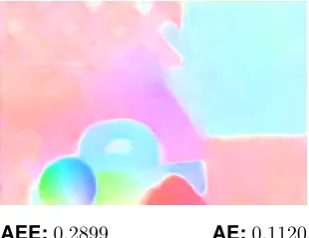
Since the architecture of FlowNet2.0 (Fig. 4.2) contains multiple components which all individually compute the optical flow as well we can look at the in-termediate results after each component. The output of FlowNet2.0 is a direct combination of two different components, one responsible for the large displace-ments and one for the short displacedisplace-ments. The component responsible for large displacements is a

chain of smaller components is indicated by FlowNet-CSS (Fig. 5.4) and the other component which is responsible for the smaller displacements is called FlowNet-SD (Fig. 5.5). We can see that these components also produce a pretty decent result if we let them work on their own.

AEE:0.2899 AE:0.1120

Figure 5.4: FlowNet-CSS

AEE:0.2408 AE:0.0906

Figure 5.5: FlowNet-SD

28 CHAPTER 5. TESTING

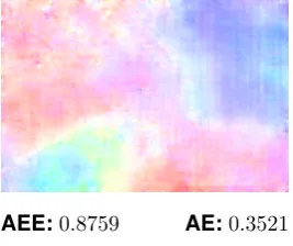
they produce come nowhere near the ground-truth.

AEE:0.8617 AE:0.3343

Figure 5.6: FlowNet-C

AEE:0.8759 AE:0.3521

Figure 5.7: FlowNet-S

However using two of these components, which perfrom really badly on their own, in succession gives us already pretty decent results as can be seen in the following figures (Fig. 5.8 and Fig. 5.9). The FlowNet-ss network from Fig. 5.9 even uses two components FlowNetS which were reduced in size by a factor 3

8.

AEE:0.3430 AE:0.1401

Figure 5.8: FlowNet-CS

AEE:0.5301 AE:0.2089

Figure 5.9: FlowNet-ss

5.3.2 Performance

We tested the FlowNet2.0 model on the Middlebury dataset [5] containing 8 image pairs and a subset of the Sintel dataset [7]. This dataset contains 23 scenes, we tested the FlowNet2.0 model on the first image pair of every scene. The results of these tests can be seen in Table 5.1. The difference between the clean and final version of Sintel is that in the final version effects like fog and motion blur are added.

AEE AE

Middlebury 0.3556 0.0526 Sintel clean 1.5312 0.0602 Sintel final 2.5728 0.1058

5.3. DEEPLEARNING 29

5.3.3 Robustness against noise

In order to test how robust the FlowNet2.0 model is we tested it on some images to which some gaussian noise was added. In Fig. 5.10 can be seen how the deep learning model of FlowNet2.0 performed on the RubberWhale image pair.

σ

:0

σ

:0

AEE:0.1873AE:0.0717

0.025

0.025

AEE:0.1991AE:0.0758

0.05

0.05

AEE:0.2425AE:0.0933

0.1

0.1

AEE:0.3340AE:0.1237

0.15

0.15

AEE:0.3976AE:0.1434

0.2

0.2

AEE:0.5736AE:0.2233

0.25

0.25

AEE:0.8210AE:0.3424

0.3

0.3

AEE:0.8259AE:0.3498

0.35

0.35

AEE:1.0564AE:0.4614

0.4

0.4

AEE:1.0906AE:0.4816

0.5

0.5

AEE:1.0694AE:0.4680

0.6

0.6

AEE:1.1551AE:0.5187 Figure 5.10: The output of FlowNet2.0 for image pairs to which gaussian noise was

added with different values for the varianceσ.

Figure 5.11:Image for σ= 0.2.

We see that the FlowNet2.0 model handles small levels of noise really well. Even for a noise level of 0.2 the solution is not that bad

30 CHAPTER 5. TESTING

In Table 5.2 the FlowNet2.0 model is tested on the same datasets as in Table 5.1 but with a certain amount of added gaussian noise.

Middlebury Sintel clean Sintel final

σ AEE AE AEE AE AEE AE

0 0.356 0.053 1.531 0.060 2.573 0.106 0.025 0.385 0.056 1.510 0.069 2.413 0.112 0.05 0.435 0.064 1.434 0.075 2.3876 0.107

Table 5.2: Performance of FlowNet2.0 on data with noise.

One thing which stands out in Table 5.2 is that for both the Sintel datasets the AEE gets smaller as noise is added. This is mostly due to one particular image pair in the dataset, this image pair is displayed in Fig. 5.12.

Figure 5.12: Image pair [7].

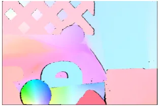
The computation of the optical flow of the uniform region in the bottom of this image pair is difficult. This results in solutions which are very different from the ground-truth as can be seen in Fig. 5.13. As we add noise, the errors at the bottom of the image get less extreme and hence the error measures get smaller.

GT

GT

Ground-Truth flow.

σ

:0

σ

:0

AEE:10.926 AE:0.2085

0.025

0.025

AEE:9.3077 AE:0.2188

0.05

0.05

AEE:5.6519 AE:0.2986 Figure 5.13: The output of FlowNet2.0 for the image pair from Fig. 5.12 to which

5.4. COMPARISON 31

The error measures displayed in Fig. 5.11 are also really large compared to the average of the dataset, so it was skewing the average performance as well. When we leave the image pair from Fig. 5.12, the only extreme outlier, out of the evaluation, we get the following results:

Sintel clean Sintel final

σ AEE AE AEE AE

0 1.104 0.053 2.069 0.085 0.025 1.156 0.063 2.177 0.096 0.05 1.243 0.065 2.272 0.101

Table 5.3: Performance of FlowNet2.0 on data with noise.

In Table 5.3 we can see that the FlowNet2.0 handles small levels of noise pretty well. Also if we compare the errors on the Sintel clean dataset to the errors on the Sintel final dataset, we see that the model apparently has more difficulties handling the effects added in Sintel final than small levels of noise.

5.4 Comparison

To compare the different approaches somewhat fairly we made some changes to the data sets to compensate for the limitations of our variational models. They were all turned into grayscale images, since our implementation of the variational models can not handle color. Also to compensate for the fact that our variational models do not account for large displacements, we scaled the ground-truth flow down to a maximum magnitude of 1. Using this downscaled ground-truth flowvˆgt we created a

new image pair through bilinear interpolation. The data from the first image u(x,1)

remained the same and for the second image we used the interpolation ofu(x+ˆvgt,1)

instead ofu(x,2).

5.4.1 Performance

In Fig. 5.14 we can see how well the different models perform on the interpolated dataset we just described. We can see that of all our variational implementations the L1-TV/TV model performs the best on theRubberWhale image pair, just barely

32 CHAPTER 5. TESTING

L1-TV

L1-TV

AEE:0.2098AE:0.1033

L1-L2

L1-L2

AEE:0.2339AE:0.1148

L1-TV/L2

L1-TV/L2

AEE:0.2467AE:0.1206

L1-TV/TV

L1-TV/TV

AEE:0.2095AE:0.1032

L2-TV

L2-TV

AEE:0.2216AE:0.1086

L2-L2

L2-L2

AEE:0.2510AE:0.1230

L2-TV/L2

L2-TV/L2

AEE:0.3396AE:0.1674

L2-TV/TV

L2-TV/TV

AEE:0.2989AE:0.1469

FN2.0

FN2.0

AEE:0.1353AE:0.0701

FN-CSS

FN-CSS

AEE:0.1685AE:0.0869

FN-SD

FN-SD

AEE:0.2061AE:0.1043

5.4. COMPARISON 33

5.4.2 Robustness against noise

In Table 5.4 we compared the robustness of the deep learning implementation with that of the variational models.

Middlebury

0 0.025 0.05

AEE AE AEE AE AEE AE

FlowNet2.0 0.178 0.085 0.216 0.102 0.267 0.125 L1-TV 0.473 0.221 0.630 0.305 0.760 0.380 L1-L2 0.489 0.232 0.643 0.313 0.762 0.383 L2-TV 0.330 0.146 0.742 0.363 1.056 0.511 L2-L2 0.343 0.152 0.747 0.375 0.932 0.479 L1-TV/L2 0.450 0.212 0.625 0.302 0.758 0.380 L1-TV/TV 0.541 0.263 0.678 0.338 0.789 0.403 L2-TV/L2 0.697 0.269 1.769 0.602 2.124 0.664 L2-TV/TV 0.949 0.364 1.791 0.609 2.140 0.667

Table 5.4: Middlebury

In Table 5.4 we again see that the variational models perform very poorly compared to the deep learning method. Although the deep learning methods are definitely out-performing the variational models, there are two factors which skew these results. Firstly the stopping condition of the algorithm was set at a relatively low amount, namely maximum 1000 iterations. Most of the time the algorithm is not fully con-verged by this time, but to keep the total runtime of the test at a reasonable limit, we could not set it much higher. We see that the L2-TV model is the best performing variational implementation, but its low error measures could also just indicate that it converges the fastest. Secondly, the parameter α was not as optimized as it could have been. We ran some tests on one image pair, and used the best performingα’s on the whole dataset. For the images with noise we setα to a slightly higher value in the hope of getting better results.

Another thing which stands out, is that the models with a L2 data term handle

noise significantly worse than the ones with a L1 data term. This is what we

ex-pected. As we mentioned in subsection 3.1.1, the L1 data term is more robust to

Chapter 6

Conclusions and recommendations

6.1 Conclusions

An upside of variational models is its theoretical foundation. This theoretical founda-tion makes it easier to understand the performance of these models. One example of this is that we know that theL2 dataterm is not that robust against noise, so we

know what needs to be changed to improve this. Comparing this to deep learning methods we see that this does not happen as often for these methods. These mod-els can generally only be improved through just trying several things and see which works best. The lack of theoretical foundation for deep learning methods makes it hard to predict which choices will work well and which will not.

On the other hand deep learning methods perform impressively well, the deep learning implementation of FlowNet2.0 [14] outperforms our implementations of vari-ational methods by a large margin. It is especially surprising that the training data apparently does not need to be highly realistic, artificial image data which is created in a fairly simple way, is already enough to get really accurate solutions. Another upside of deep learning is that it computes the solution really fast. Where the varia-tional models take minutes to converge, the FlowNet2.0 model can give the solutions in under a second. The computation time is traded in for a lot of training time, which does require a lot of GPU-power.

6.2 Recommendations

For the variational approach we used an implementation which is definitely not repre-sentative of the state-of-the-art variational methods. Our implementation has several weaknesses.

Firstly our implementation can not handle large displacements. We mentioned in section 2.2 how the displacement needs to be small if we wanted the optical flow

36 CHAPTER 6. CONCLUSIONS AND RECOMMENDATIONS

constraint to work. This problem could be solved by a strategy mentioned in [4], which involves computing the flow on several scaled down versions of the images and formation of image pyramids, which is mentioned in [4]. The top of the pyramid contains the images which are scaled down the most and the original images are at the bottom. Then starting at the top we can compute the optical flow and use it to warp the second image in the next layer. The warping compensates for the larger displacements detected in the previous layer, so after the warping only small displacements should remain. This can be repeated until finally the optical flow of the original image can be computed.

Bibliography

[1] [Online]. Available: http://i21www.ira.uka.de/image sequences/

[2] F. Becker, S. Petra, and C. Schn¨orr, “Optical flow,” inHandbook of Mathematical Methods in Imaging, 2015.

[3] A. Bruhn, J. Weickert, and C. Schn¨orr, “Lucas/kanade meets horn/schunck: Combining local and global optic flow methods,” International Journal of Com-puter Vision, vol. 61, pp. 211–231, 2005.

[4] M. Burger, H. Dirks, and L. Frerking, “On optical flow models for variational motion estimation,”CoRR, vol. abs/1512.00298, 2015.

[5] S. Baker, D. Scharstein, J. P. Lewis, S. Roth, M. J. Black, and R. Szeliski, “A database and evaluation methodology for optical flow,”Int J Comput Vis, vol. 92,

pp. 1–31, 2011.

[6] A. Geiger, P. Lenz, C. Stiller, and R. Urtasun, “Vision meets robotics: The kitti dataset,”International Journal of Robotics Research (IJRR), 2013.

[7] D. J. Butler, J. Wulff, G. B. Stanley, and M. J. Black, “A naturalistic open source movie for optical flow evaluation,” inEuropean Conf. on Computer Vision (ECCV), ser. Part IV, LNCS 7577, A. Fitzgibbon et al. (Eds.), Ed.

Springer-Verlag, Oct. 2012, pp. 611–625.

[8] B. K. Horn and B. G. Schunck, “Determining optical flow,” Artificial Intelligence, vol. 17, no. 1, pp. 185 – 203, 1981. [Online]. Available:

http://www.sciencedirect.com/science/article/pii/0004370281900242

[9] A. Chambolle and T. Pock, “A first-order primal-dual algorithm for convex prob-lems with applications to imaging,”Journal of Mathematical Imaging and Vision,

vol. 40, pp. 120–145, 2011.

[10] L. Frerking, “Variational methods for direct and indirect tracking in dynamic imaging,” 2016.

38 BIBLIOGRAPHY

[11] N. Huttinga, “Insights into deep learning methods with application to cancer imaging,” 2017.

[12] Y. Jia, E. Shelhamer, J. Donahue, S. Karayev, J. Long, R. Girshick, S. Guadar-rama, and T. Darrell, “Caffe: Convolutional architecture for fast feature embed-ding,”arXiv preprint arXiv:1408.5093, 2014.

[13] A. Dosovitskiy, P. Fischer, E. Ilg, P. H¨ausser, C. Hazirbas, V. Golkov, P. van der Smagt, D. Cremers, and T. Brox, “Flownet: Learning optical flow with convo-lutional networks,” 2015 IEEE International Conference on Computer Vision (ICCV), pp. 2758–2766, 2015.

[14] E. Ilg, N. Mayer, T. Saikia, M. Keuper, A. Dosovitskiy, and T. Brox, “Flownet 2.0: Evolution of optical flow estimation with deep networks,” in IEEE Conference on Computer Vision and Pattern Recognition (CVPR), Jul 2017. [Online].

Available: http://lmb.informatik.uni-freiburg.de//Publications/2017/IMKDB17

Appendix A

Appendix A

A.1 MATLAB implementation of variational models

1 f u n c t i o n [ v ] = OpticalFlow ( image1 , image2 , alpha , data , reg ,

m a x i t e r a t i o n s , tolerance , theta , x s t a r t , y s t a r t )

2 %Image s i z e

3 [ y , x ] = s i z e( image1 ) ;

4 xy = x ∗ y ;

5

6 %Nabla

7 %( i +1) − ( i−1)

8 [ d1x , d1y ] = GradientMatrix1 ( x , y ) ; 9 %( i +1) − ( i )

10 [ d2x , d2y ] = GradientMatrix2 ( x , y ) ; 11

12 %Image D e r i v a t i v e s

13 uy = d1x∗image1 ( : ) ; 14 ux = d1y∗image1 ( : ) ;

15 ut = image2 ( : )−image1 ( : ) ; 16

17 %a square

18 a s = ux . ˆ 2 + uy .ˆ2+1 e−8; 19

20 %Matrices f o r b u i l d i n g operator K

21 O = sparse( xy , xy ) ;

22 I = speye( xy , xy ) ;

23

24 %Data−term

40 APPENDIXA. APPENDIX A

25 d a t a o p t i o n s = {’ L2 ’ , ’ L1 ’};

26 switch data

27 case d a t a o p t i o n s ( 1 ) 28 %Data−term : L2

29 proxG = @( x , tau ) prox L2 data ( x , tau ) ; 30

31 case d a t a o p t i o n s ( 2 ) 32 %Data−term : L1

33 proxG = @( x , tau ) prox L1 data ( x , tau ) ; 34

35 otherwise

36 disp( ’ E r r o r : i n v a l i d Data−term ’)

37 end

38

39 %R e g u l a r i z a t i o n−term

40 r e g o p t i o n s = {’ L2 ’ , ’TV ’ , ’TV / L2 ’, ’TV / TV ’};

41 switch reg

42 case r e g o p t i o n s ( 1 )

43 %R e g u l a r i z a t i o n−term : L2

44 x s i z e = 2;

45 y s i z e = 4;

46 proxFS = @( y , sigma ) prox L2 S ( y , sigma ) ;

47 K = [ d2x O;

48 d2y O;

49 O d2x ;

50 O d2y ] ;

51 Ks = K ’ ;

52

53 case r e g o p t i o n s ( 2 )

54 %R e g u l a r i z a t i o n−term : TV

55 x s i z e = 2;

56 y s i z e = 4;

57 proxFS = @( y , sigma ) prox TV S ( y , sigma ) ;

58 K = [ d2x O;

59 d2y O;

60 O d2x ;

61 O d2y ] ;

62

A.1. MATLAB IMPLEMENTATION OF VARIATIONAL MODELS 41

64

65 case r e g o p t i o n s ( 3 )

66 %R e g u l a r i z a t i o n−term : TV / L2

67 x s i z e = 4;

68 y s i z e = 4;

69 proxFS = @( y , sigma ) prox TV S ( y , sigma ) ;

70 K = [ d2x O −I O;

71 d2y O −I O;

72 O d2x O −I ;

73 O d2y O −I ] ;

74 Ks = K ’ ;

75 w extension = t r u e ;

76

77 case r e g o p t i o n s ( 4 )

78 %R e g u l a r i z a t i o n−term : TV / TV

79 x s i z e = 4;

80 y s i z e = 8;

81 proxFS = @( y , sigma ) prox TV S ( y , sigma ) ;

82 K = [ d2x O −I O;

83 d2y O −I O;

84 O d2x O −I ;

85 O d2y O −I ;

86 O O d2x O;

87 O O d2y O;

88 O O O d2x ;

89 O O O d2y ] ;

90 Ks = K ’ ;

91 w extension = f a l s e ; 92

93 otherwise

94 disp( ’ E r r o r : I n v a l i d R e g u l a r i z a t i o n Term ’)

95 end

96

97 %Other Parameters

98 i f x size>2 99 sigma = 0 . 5 ; 100 tau = 0 . 2 5 ;

101 else

42 APPENDIXA. APPENDIX A

103 tau = 0 . 2 ;

104 end

105

106 %I n i t i a l Values

107 i f nargin>8 108 x = x s t a r t ;

109 else

110 x = zeros( x s i z e∗xy , 1 ) ;

111 end

112 i f nargin>9 113 y = y s t a r t ;

114 else

115 y = zeros( y s i z e∗xy , 1 ) ;

116 end

117 x bar = x ;

118 dx = I n f ;

119 i t e r a t i o n s = 0; 120

121 %Main Loop

122 while i t e r a t i o n s<m a x i t e r a t i o n s && dx>t o l e r a n c e 123 x o l d = x ;

124

125 y = proxFS ( y + sigma∗K∗x bar , sigma ) ; 126 x = proxG ( x − tau ∗ Ks ∗ y , tau ) ; 127 x bar = x + t h e t a ∗ ( x − x o l d ) ; 128

129 dx = sum(abs( x ( 1 : 2∗xy ) − x o l d ( 1 : 2∗xy ) ) ) / xy ; 130 i t e r a t i o n s = i t e r a t i o n s + 1;

131 end

132

133 %Resize x

134 v = reshape( x ( 1 : 2∗xy ) , [s i z e( image1 ) , 2 ] ) ; 135

136 %Functions

137 f u n c t i o n [ x ] = prox L1 data ( xhat , tau )

138 rho = ut + ux .∗xhat ( 1 : xy ) + uy .∗xhat ( xy +1:2∗xy ) ; 139

A.1. MATLAB IMPLEMENTATION OF VARIATIONAL MODELS 43

142 cond2 = rho > tau ∗ a s ; 143 val2 = −val1 ;

144 cond3 = 1−cond1−cond2 ;

145 val3 = −[ rho ; rho ] .∗ [ ux . / a s ; uy . / a s ] ; 146

147 x = xhat ( 1 : 2∗xy ) + val1 .∗ [ cond1 ; cond1 ] + val2 .∗ [

cond2 ; cond2 ] + val3 .∗ [ cond3 ; cond3 ] ;

148 i f ( x size>2)

149 i f w extension

150 w = ( xhat (2∗xy +1:end) ) / ( 1 + tau∗alpha ( 2 ) ) ;

151 x = [ x ;w ] ;

152 else

153 x = [ x ; xhat (2∗xy +1:end) ] ;

154 end

155 end

156 end

157 f u n c t i o n [ x ] = prox L2 data ( xhat , tau ) 158 a1 = 1 + tau∗ux .∗ux ;

159 a2 = tau ∗ ux .∗uy ; 160 a3 = 1 + tau∗uy .∗uy ;

161 b1 = xhat ( 1 : xy ) − tau∗ux .∗ut ;

162 b2 = xhat ( xy +1:2∗xy ) − tau∗uy .∗ut ; 163

164 v1 = ( a3 .∗b1−a2 .∗b2 ) . / ( a1 .∗a3−a2 .ˆ2+1 e−8) ; 165 v2 = ( a1 .∗b2−a2 .∗b1 ) . / ( a1 .∗a3−a2 .ˆ2+1 e−8) ; 166 x = [ v1 ; v2 ] ;

167 i f ( x size>2)

168 i f w extension

169 w = ( xhat (2∗xy +1:end) ) / ( 1 + tau∗alpha ( 2 ) ) ;

170 x = [ x ;w ] ;

171 else

172 x = [ x ; xhat (2∗xy +1:end) ] ;

173 end

174 end

175 end

176 f u n c t i o n [ x ] = prox TV S ( xhat , ˜ ) 177 i s o t r o p i c = t r u e ;

178 i f x size>2

44 APPENDIXA. APPENDIX A

180 else

181 alpha = alpha ;

182 end

183 i f ˜ i s o t r o p i c 184 %A n i s o t r o p i c

185 x = max(−alpha , (min( alpha , xhat ( 1 : 4∗xy ) ) ) ) ;

186 else

187 %I s o t r o p i c

188 xnorm = reshape( xhat ( 1 : 4∗xy ) , [ xy , 4 ] ) ; 189 xnorm1 = (sum( xnorm ( : , 1 : 2 ) . ˆ 2 , 2 ) ) . ˆ 0 . 5 ; 190 xnorm2 = (sum( xnorm ( : , 3 : 4 ) . ˆ 2 , 2 ) ) . ˆ 0 . 5 ; 191 xnorm = [ xnorm1 ; xnorm1 ; xnorm2 ; xnorm2 ] ; 192 x = xhat ( 1 : 4∗xy ) . / (max( 1 , xnorm / alpha ) ) ;

193 end

194 i f y size>4

195 alpha = alpha ( 2 ) ;

196 i f ˜ i s o t r o p i c 197 %A n i s o t r o p i c

198 w = max(−alpha , (min( alpha , xhat (4∗xy +1:end)

) ) ) ;

199 else

200 %I s o t r o p i c

201 xnorm = reshape( xhat (4∗xy +1:end) , [ xy , 4 ] ) ; 202 xnorm1 = (sum( xnorm ( : , 1 : 2 ) . ˆ 2 , 2 ) ) . ˆ 0 . 5 ; 203 xnorm2 = (sum( xnorm ( : , 3 : 4 ) . ˆ 2 , 2 ) ) . ˆ 0 . 5 ; 204 xnorm = [ xnorm1 ; xnorm1 ; xnorm2 ; xnorm2 ] ;

205 w = xhat (4∗xy +1:end) . / (max( 1 , xnorm / alpha ) ) ;

206 end

207 x = [ x ;w ] ;

208 end

209 end

210 f u n c t i o n [ x ] = prox L2 S ( xhat , tau ) 211 x = xhat / ( 1 + tau / alpha ) ;

212 end