R E S E A R C H
Open Access
Linear IC detectors for low to medium SNR
ill-conditioned communication systems with
unknown noise variance
Abdelouahab Bentrcia
1*and Saleh A Alshebeili
1,2Abstract
In this paper, we introduce two new linear parallel interference cancellation (LPIC) detectors that are suitable for low to medium signal-to-noise ratio ill-conditioned communication systems and do not require knowledge of the noise variance but perform close to the linear minimum mean square error detector, which needs such information. Particularly, we focus in this work on fast linear parallel interference cancellation detectors that are asymptotically equivalent to the steepest descent and conjugate gradient algorithms, respectively, and show that they exhibit a spectral filtering property and semi-convergence behavior. Consequently, a deterministic stopping rule to stop the LPIC iterations that is independent of the noise level (known as the L-curve method) is investigated and tested. Simulation results are presented to support our theoretical findings.
Keywords:Linear; PIC; Regularization; Semi-convergence; Linear MMSE; L-curve
1. Introduction
The capacity of the third-generation cellular systems and optical networks using optical CDMA (OCDMA) technol-ogy is mainly limited by the multi-access interference (MAI) [1]. Other systems suffer from other types of in-terference such as the inter-carrier inin-terference (ICI) in orthogonal frequency division multiple access (OFDMA) and inter-antenna interference (IAI) in multiinput multi-output (MIMO) systems, just to name a few [1].
In 4G and beyond wireless communication systems, the problem of interference is becoming of increasing importance because cells are getting smaller and condensed (i.e., femto-cells) and new technologies that cause additional interference are introduced. For example, relay nodes are proposed to increase coverage and allow cooperative com-munication; however, they also bring additional interfer-ence into the network [2].
To combat these different types of interferences, vari-ous interference cancellation and multiuser detection al-gorithms are proposed. Multiuser detectors (MUDs) are mainly introduced to reduce the effect of interference in
wireless/wired systems and consequently to boost the sys-tem capacity and throughput. Many multiuser detectors were developed in the literature and have found applica-tions in various wireless/wired systems such as OCDMA, MIMO-OFDM, and MIMO-UWB, just to name a few [1-5]; however, due to the fact that the capacity of CDMA systems is essentially limited by MAI, a large part of the lit-erature of MUDs focused on systems based on the CDMA technology.
The decorrelating detector is an effective multiuser de-tector to eliminate interference. It is also an important building block for nonlinear multiuser detectors. It enjoys several desirable features such as: (1) complete removal of interference and (2) independence of noise level informa-tion. The latter is very important in situations where the estimation of the noise variance is not possible or not ac-curate. This is the case where the noise term includes in addition to thermal noise, other types of background noise such as co-channel interference which may change signi-ficantly with time/frequency (particularly in frequency-hopping systems) and its variance can be considered as unknown to the receiver [6,7].
However, the decorrelating detector suffers from two drawbacks: (1) Its relatively high computational complex-ity which is of the order of O(N3) [1], where N in the * Correspondence:[email protected]
1
Prince Sultan Advanced Technologies Research Institute (PSATRI), King Saud University, P.O. Box 800, Riyadh 11421, Saudi Arabia
Full list of author information is available at the end of the article
dimension of the system's cross-correlation matrix and (2) noise enhancement effect. Therefore, the challenge is to maintain the advantages of the decorrelating detector and overcome its deficiencies, that is, to lower its computational complexity and combat the noise enhancement effect but without requiring the knowledge of the noise variance, like the linear minimum mean square error (LMMSE) detector.
Recent results reported in [8] proved the semi-convergence behavior of the conventional linear parallel interference cancellation (LPIC) detector and showed that early stopping rules can be used to combat the noise en-hancement effect. They used the Morozov discrepancy rule to stop the LPIC iterations prior to final convergence in order to avoid noise magnification. However, the con-ventional LPIC detector is very slow and may require a very large number of stages to converge especially for ill-conditioned communication systems. Moreover, the Mor-ozov discrepancy rule requires the noise level information and therefore cannot be used in many practical settings.
Building up on these results, a twofold approach is proposed in this work to overcome the drawbacks of the decorrelator detector cited above. First, we employ fast linear interference cancellation detectors to reduce its computational complexity, and then, we make use of an early stopping technique (known as the L-curve method) that does not require noise level information to reduce the noise enhancement effect [9]. Up to our knowledge, this is the first work that investigates the possible use of these early stopping rules that do not require noise level information in the communication field. Preliminary re-sults are promising and suggest that more improvements and extensions can be made.
The organization of this paper is as follows: in Section 2, a simplified system model of the OFDMA uplink that will be used throughout this work is briefly described. In Section 3, the decorrelator detector's solution is analyzed and some of the regularization techniques that are used to overcome its drawbacks are detailed. Section 4 briefly de-scribes the fast LPIC detectors and shows their spectral fil-tering property. Section 5 analyzes the semi-convergence behavior of the LPIC detector and then investigates the L-curve stopping rule and shows how it can be applied to the LPIC detector. Section 6 supports the theoretical find-ings by a number of simulations. Finally, Section 7 con-cludes the paper with some results and recommendations.
2. System model
For illustration purposes only and similar to [8], we
con-sider an uplink OFDMA system where K users transmit
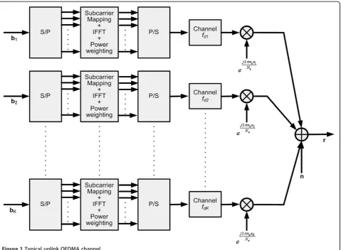
simultaneously over a Rayleigh fading channel using quad-rature phase-shift keying (QPSK). Particularly, we consider in this work the effect of ICI due to the misalignment of the carrier frequencies and to the Doppler shifts of differ-ent users such as in the uplink of the mobile WIMAX
(IEEE 802.16 Wireless MAN standard) [10]. This is depicted in Figure 1.
In this work, we consider the interleaved subcarrier al-location scheme because it is well known that this scheme suffers the most from ICI compared to other subcarrier allocation schemes [11].
An OFDM symbol consisting ofNu samples with
sam-pling timeTuwhere Nu is the total number of data
sam-ples is transmitted using N orthogonal subcarriers.
Without loss of generality, we assume that the total num-ber of subcarriers of the IFFT matrix Ψ with elements Ψnu;n¼
1 ffiffiffiffiffi Nu
p ej2πNunun, 1≤nu≤Nu, and 1≤n≤N is divided
equally among all users; therefore, the total number of subcarriers per user isNk=N/K.
Based on Figure 1, the received signalr(m) at themth OFDM symbol is expressed in vector–matrix form as:
rð Þ ¼m Ψ~Hð Þm Abð Þ þm nð Þm
¼Ψ~~ð Þm bð Þ þm nð Þm; ð1Þ
where
Ψ~ ¼Ψ∘ 11;Nk⊗Ε
is a combination of the IFFT matrix
Ψ and the normalized carrier frequency offset
(NCFO) matrixE. Here, ○and⊗denote the Schur
and Kronecker products, respectively, and 11;Nk
denotes a 1-by-Nk vector of ones. The NCFO
matrix can be partitioned as Ε¼½ε1 ε2 ⋯ and Δf is the subcarrier spacing.
H(m) is the matrix of Rayleigh fading coefficients and it is given by: Hð Þ ¼m diagðH1ð Þm H2ð Þm ⋯
Hnkð Þm ⋯ HNkð Þ Þm , where Hnkð Þ ¼m diag
h1;nk
ð ð Þm h2;nkð Þm⋯hk;nkð Þm ⋯ hK;nkð Þ Þm .
A is the matrix of amplitudes and it is given by:
A¼diagðA1 A2 ⋯ Ank ⋯ ANk Þ, where
Ank ¼ diag að 1;nk a2;nk ⋯ ak;nk ⋯ aK;nk Þ:It
is used to weight the signals of different users with different powers to simulate near-far scenarios.
b(m) is the vector of transmitted data symbols and it can be partitioned as: bð Þ ¼m ½b1ð Þm b2ð Þm ⋯ identically distributed additive white Gaussian noise samples with zero mean and varianceρ2.
the IFFT, the NCFO, the channel gain, and power weight-ing matrices, respectively. To simplify the notations, we drop in all subsequent equations the OFDM symbol index mfrom all matrices and vectors used in Equation (1).
3. Regularization techniques for combating the noise enhancement effect
The decorrelator detector (known also as the zero-forcing detector) is a fundamental detector that allows complete removal of the interference, and it results from solving the following least square minimization problem:
b: min
b∈ℂN r−Ψ~~b
2
2 ð2Þ
which yields
yDEC¼Ψ~~†r¼ Ψ~~HΨ~~
−1~~
ΨH
r; ð3Þ
where Ψ~~† is the pseudo-inverse of the system matrix Ψ~~
andΨ~~HΨ~~ is the ICI matrix.
Using the singular value decomposition (SVD), the system matrixΨ~~ can be decomposed as:
~~
Ψ¼UΣVH; ð4Þ
whereUandVare theN-by-NandN-by-Nunitary matri-ces that represent the left and right singular vectors of Ψ~~, respectively, andΣis anN-by-Ndiagonal matrix with
ele-mentsσk, 1≤n≤Nthat represent the singular values of Ψ.~~ In addition, the unitary matricesUandVcan be partitioned
as U¼½u1 u2 ⋯ un ⋯ uN and U¼½v1 v2⋯
vn ⋯ vN, respectively. Therefore, Equation (3) can be
written in terms of the SVD ofΨ~~ as:
yDEC¼Ψ~~†r¼VΣ−1UHr¼X
N
n
uH nr
σn
vn: ð5Þ
Consequently, its norm can be written as:
yDEC
2¼
ffiffiffiffiffiffiffiffiffiffiffiffiffiffiffiffiffiffiffiffiffiffiffiffiffi XN
n
uH nr
σn
2
v u u
t : ð6Þ
It is clear from Equation (6) that as long as uH nr <σn
for large n, the norm of yDEC will not go unbounded. This is what is known as the Picard condition [12]; how-ever, due to the contamination of the received signal with noise, the Fourier coefficients uH
nr do not decay
monotonically to zero, instead they settle at certain level
ρ while the singular values decay to zero. Therefore, all singular values belowρcontribute to the noise enhance-ment effect.
To get rid of the small singular values that may cause the violation of the discrete Picard condition, the decorr-elator detector's solution is modified by introducing a fil-tering matrixFsuch that:
yREG¼X
whereyREGis the regularized solution andFis an N-by-Ndiagonal matrix with elementsfn, satisfying:
fn≃ 1 if σnis large
0 if σnis small ;
1≤n≤N:
ð8Þ
Consequently, these factors filter out solution compo-nents pertaining to small singular values.
The most straightforward regularization technique is known as the truncated SVD (TSVD) and is given by [13]:
Therefore, the filter factors for this regularization scheme can be expressed as:
fn≃ 1 if n≤n
0
0 if n>n0 ; 1≤n≤N:
ð10Þ
This regularization technique is known also as spectral cutting technique and relies on cutting off all solution components under a certain threshold determined by the discrete regularization parametern’.
Another regularization scheme is known as the Tikhonov regularization technique, and it relies on modifying the least square minimization problem in Equation (2) by pen-alizing solutions of large norm, that is, [13]:
b: min
where η is the regularization parameter that determines the amount of penalization the solution norm undergoes. The rationale behind this is that from one side we want to make the residual small as in the conventional least squares, but at the same time, we want to obtain
meaningful solutions and exclude those with large norms as they are usually contaminated with noise. Fortunately, Equation (11) has a closed form solution and is given by:
yTik¼ Ψ~~HΨ~~ þη2I
−1~~
ΨH
r: ð12Þ
Note that if the regularization parameter is equal to the noise level ρ, then the Tikhonov solution equals to the linear minimum mean square error (LMMSE) solu-tion. The filter factors of the Tikhonov regularization scheme are given by:
fn¼ σ
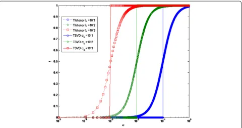
The filter factors of the Tikhonov regularization scheme behaves like a smooth low pass filter of the solu-tion terms damping solusolu-tion components pertaining to singular values less than η. The filter factors of the TSVD and the Tikhonov regularization schemes are depicted in Figure 2.
Another category of regularization methods is
regularization by early stopping [13], that is, apply an it-erative method to the least square problem of Equation (2) and stop the iterations prior to convergence. This is motivated by the fact that for ill-conditioned systems, linear iterative methods exhibit a semi-convergence property and tend to generate good solutions at early it-erations but after a certain number of itit-erations, the noise starts dominating the solution and the perform-ance of the iterative method worsens.
Many linear interference cancellation schemes have been shown to be equivalent to certain iterative methods [1], and therefore, they tend to have the same semi-convergence behavior for ill-conditioned systems. There-fore, linear IC detectors equipped with efficient early stopping mechanisms that do not require the noise level information can be used to implement a low-complexity decorrelating detector that resists noise amplification without requiring knowledge of the noise level. In the following, we focus on the LPIC detector and use it as an iterative regularizing scheme to achieve two simultan-eous objectives: low-complexity and resistance to noise enhancement.
such as the steepest descent and the conjugate gradient methods are now introduced. The residual norm stee-pest descent (RNSD) and conjugate gradient least squares (CGLS) methods belong to a class of iterative techniques known as non-stationary iterative methods where the weighting factor changes from one stage to another [14], that is:
ypþ1¼ypþωpdp; ð14Þ
whereωpis the step size anddpis the search direction. For RNSD, the search direction is equal to the residual error and is given by: dp¼ep¼Ψ~~
H
r−Ψ~~yp
while the
weighting factor is determined as:
ωp¼
dHpdp
dHpΨ~~HΨ~~dp
: ð15Þ
For the CGLS method, the initial search directiond0is
set to the residual error, that is,d0¼e0¼Ψ~~ H
r−Ψ~~y0
,
and then, we proceed as:
ωp¼
eHpΨ~~HΨ~~ep
dHpΨ~~HΨ~~dp
ð16Þ
and
ypþ1¼ypþωpdp: ð17Þ
Then, we updateepanddpas:
epþ1¼ep−ωpΨ~~dp ð18Þ
and
dpþ1¼Ψ~~ H
epþ1þβpþ1dp; ð19Þ
where
βpþ1¼
eHpþ1Ψ~~HΨ~~epþ1
eH pΨ~~
H~~
Ψep
: ð20Þ
To determine the filter factors of the RNSD, it can be shown without loss of generality that if y0= 0, then yp can be written in the following form [14]:
ypþ1¼TSDp Ψ~~HΨ~~
~~ ΨH
r; ð21Þ
where the polynomialTSD
p is defined as:
TSD
p ð Þ ¼θ TSDp−1ð Þ þθ ωp 1−θTSDp−1ð Þθ
ð22Þ
andTSD−1ð Þ ¼θ 0.
SubstitutingΨ~~ ¼UΣVH into Equation (21), we obtain
ypþ1¼VFΣ−1UHr¼ XN
n¼1
σ2 nTSDp σ2n
uHnr
σn
whereF isN-by-Ndiagonal matrix with elementsfp+1, n given by:
fpþ1;n¼σ2nTSDp σ2n ; 1≤n≤N: ð24Þ
Following the same approach used for the RNSD, the filter factors of the CGLS can be found as:
fpþ1;n¼σ2nTCGp σ2n ; 1≤n≤N; ð25Þ
where the polynomialTCGp for the CGLS is defined as:
TCGp ð Þ ¼θ 1−ωpθþ
ωpβp−1
ωp−1
TCGp−1ð Þθ −ωpβp−1
ωp−1
TCGp−2ð Þθ
þωp
ð26Þ
andTCG−1ð Þ ¼θ 0 andTCG0 ð Þ ¼θ ω0
Finally, the average BER of the LPIC detector based on the RNSD/CGLS iterative methods is given by (see Appendix for derivation):
Pbð Þ ¼p
1 N
XN
n¼1
1 2N−1
X
allb bn¼1
Q g
H p;nΨ~~b
ρ ffiffiffiffiffiffiffiffiffiffiffiffiffiffiffigH p;ngp;n q 0 B @
1 C
A; ð27Þ
where GH
p ¼TSDp Ψ~~ H~~
Ψ
~~ ΨH
for the LPIC detector
based on the RNSD and GHp ¼TCGp Ψ~~HΨ~~
~~ ΨH
for
the LPIC detector based on the CGLS and Gp=
[gp,1 gp,2⋯ ⋯gp,n⋯gp,N].
5. Semi-convergence behavior of the LPIC detector and early stopping using the L-curve method
The LPIC detector exhibits a semi-convergence prop-erty where it reaches a BER that is better than that achieved at final convergence. This phenomenon has been studied in more detail in [8]. Interested readers are referred to [8] for more details. For our case, the semi-convergence property of the proposed detectors is illustrated in Figure 3. For the simulation parame-ters, we set the carrier frequency to 3.5 GHz,
signal-to-noise ratio (SNR) to 13 dB, N to 128, and K to 4
with frequency offsets (ɛ 1=−0.35,ɛ2= 0.38,ɛ3= 0.36,
ɛ 4=−0.39) and speeds 80, 120, 90, and 100 km/h,
respectively.
It is clear that the two detectors, that is, the one equivalent to the RNSD method (RNSD-LPIC) and the one equivalent to the CGLS method (CGLS-LPIC), ex-hibit a semi-convergence behavior where they reach their minimum average BER at 10 and 45 stages, re-spectively, and converge to the decorrelator detector's solution.
The RNSD-LPIC detector exhibits a slower conver-gence behavior and wide flat minimum while the CGLS-LPIC detector exhibits faster convergence and a narrow minimum.
It is difficult to analyze the semi-convergence behavior using the average BER; nevertheless, we can calculate the mean square error between the decision variable of the LPIC detector at stage (p+ 1),yp+1and the vector of
the transmitted data symbolsb, that is:
MSE ypþ1
It can be seen that the MSE can be decomposed into two components: the bias (also known as the data error) and the variance (also known as the noise error). The data error is caused by using a modified inverse of the
ICI matrixΨ~~HΨ~~ instead of the true inverse whereas the noise error is caused by the noise enhancement effect. It is evident from Equation (28) that ifF⋍I, the data error is small but the noise error is large due to the noise en-hancement effect; however, if F ⋍ 0, the noise error is small but the data error is large, and as a result, the so-lution is heavily damped and a large part of it is lost.
Therefore, a proper choice of the filtering matrix F should balance between the data and noise errors. Be-cause the amount of filtering introduced by the filtering matrix is proportional to the stage index p, a proper stopping rule needs to be devised. Many stopping rules have been developed in the literature but roughly they can be classified into three broad techniques [9]:
Methods requiring the knowledge of the exact noise level.
Methods requiring the knowledge of the approximate noise level.
Methods not requiring the knowledge of the noise level.
Due to the fact that we are assuming the absence of the noise level information, we neglect the first two categories and focus on the last one. Under this category, the most known stopping rule technique is the L-curve method [15]. This method has been used successfully in many areas such as spectroscopy, seismography, and medical imaging. The L-curve method exhibits some desirable fea-tures such as:
Does not need the noise level information. This is important for communication systems where this information is not always available or it is not accurate.
Works well under colored Gaussian noise. This is important when the additive white Gaussian noise assumption in communication systems is violated, or it becomes colored because of some signal processing operations such as matched filtering.
This method intends to balance between two conflict-ing goals: minimizconflict-ing the residual error norm and keep-ing the solution norm small. Careful inspection reveals
that the norm of the residual error r−Ψ~~yp
2 declines
sharply at early stages, and then, it flattens while the so-lution norm ‖yp‖2 increases sharply at early stages and
then it flattens. Consequently, if we plot the residual error norm versus the solution norm, we obtain an L-shaped curve with usually a distinct corner that splits the curve into two separate regions as shown in Figure 4.
Noting that the residual and the solution norms can be written in terms of the filtering factors as [13]:
r−Ψ~~yp
and
respectively. It is clear that iffp,n≈1 (at early stages), we are in the upper part of the curve. A small change infp,n leads to a larger change in f2p;n than in (1−fp,n)2; hence,
we expect ‖yp‖2 to change the most in this region, i.e.,
we expect the curve to be steep. On the other hand, if fp,n≈0 (at late stages), we are in the lower part of the curve. A small change infp,n leads to a larger change in
(1−fp,n)2 than in f2p;n; hence, we expect r−Ψ~~yp 2 to
change the most in this region, i.e., we expect the curve to be flat here.
The two regions, that is, the vertical and horizontal, are dominated by two types of errors: data error and noise error, respectively. The corner formed by the conjunction of these two regions balances between the data and noise errors, and therefore, the stage index corresponding to this corner is selected as the best regularization parameter that compromises between data and noise errors.
Many algorithms have been devised to find the corner of the L-curve [16]. The most common technique is known as the maximum curvature method. It consists of choosing the stage index that maximizes the following function:
differentiation with respect to the regularization param-eterp.
The authors in [17] suggested plotting the residual
norm versus the stage index p and noticed that this
curve usually exhibits an L-curve shape as well. For this curve, one should find the stage index that maximizes the following simplified function:
popt¼ arg max
In order to implement the above stopping rule, we have to evaluate the norm of the residual error for each OFDM symbol a certain number of stages till the L-shaped curve is obtained and calculate the curvature in-formation to ultimately determine the optimal stopping stage. This is too expensive in practice and consequently, another alternative should be sought. Fortunately, simu-lation results reveal that the optimal stage index popt is
insensitive to variations in the condition number of sys-tem matrix and is almost constant from one OFDM symbol to another, and therefore, it is sufficient to obtain poptfor a few OFDM symbols (practically in the range of
10 to 100 OFDM symbols) and then average it and use it for the rest of the OFDM symbols. This works well in practice and costs only a marginal addition to the overall LPIC computational complexity.
Another problem with the LPIC detector based on the
CGLS is that the norm of the residual error r−Ψ~~yp
2
behaves erratically for very ill-conditioned systems [14] where the norm of the residual error may increase occa-sionally and causes the maximum curvature detector to mistakenly detect the maximum curvature at the wrong stage index. To overcome this problem, we exploit the fact that the residual error decay exponentially and therefore can be fitted by a decaying exponential. The resulting exponentially fitted curve is used instead in computing the maximum curvature and hence the opti-mal stage index. This method proved to be efficient in combating the erratic behavior of the residual error norm of the LPIC detector based on the CGLS.
Lastly, the L-curve method has obviously some limita-tions as discussed in [15]. The main one is that the regu-larized solution does not converge to the true solution as the noise variance vanishes to zero. Therefore, in our application, we expect that the LPIC detector equipped with the L-curve stopping rule will work well for only a certain range of SNRs. Fortunately, this range covers low and medium SNRs where the noise enhancement effect is most prominent. More insight about this issue is given in the simulation results.
6. Computational complexity
The computational complexity of the basic LPIC de-tector with fixed step size used in [8] and the ones pro-posed here exhibit a computational complexity in the order of O(N2), namely the conjugate gradient based LPIC detector needs 4N2 +8N-1 cflopsaper iteration and the steepest descent based LPIC detector needs 4N2+6N-1 cflops per iteration, and finally, the conventional LPIC de-tector requires 2N2 +2N +1 cflops per iteration. Even though the conjugate gradient based LPIC detector ex-hibits a slightly higher computational complexity per iter-ation compared to the other detectors, it however needs the least number of iterations; this is why it is the mostly used iterative method in practice.
The L-curve method requires the following operations with the following computational complexity:
1. Norm calculation ofη(p) =‖yp‖2: 2Ncflops. 2. Norm calculation ofρð Þ ¼p r−Ψ~~yp
22Ncflops. 3. Curvature information ofκ(p): 2p-3 flops.
4. Obtaining the index of the maximum curvature:
popt ¼ arg max
1≤p≤P
ρð Þp00 ρð Þp02þ1
ð Þ32¼κð Þp
:pflops.
Total complexity forMsymbols (Min practice is between 10 to 100) is: 4MNcflops +3M(p-1) flops. On the other hand, the Morozov stopping rule relies mainly on the estimation of the noise variance. A typical noise variance estimation algorithm used in wireless communication systems and specifically within the context of spectrum sensing [18], solves a yule-walker set of equations using Levinson-Durbin algorithm and needs a complexity of 2MN2cflops [19]. It is clear from the above expressions that the
computational complexity of the L-curve early stopping method is less than that of Morozov early stopping method by an order of magnitude. Therefore, in terms of computational complexity, using the L-curve, early stopping method is much cheaper than using the Morozov early stopping method.
7. Simulation results
In the following, we evaluate the performance of the LPIC detector equipped with the L-curve stopping rule and based on the residual norm steepest descent and conjugate gradient least squares, respectively (which are referred to by RNSD-LPIC and CGLS-LPIC detectors, for conciseness).
First, we show how the L-curve method works. For this reason, we plot the norm of the residual error of both the RNSD-LPIC and CGLS-LPIC detectors for one OFDM symbol versus the stage indexp, and we plot also its curvature using Equation (32). We set the carrier
fre-quency to 3.5 GHz, SNR to 5 dB, Nto 128, andK to 4
with frequency offsets (ɛ 1=−0.35, ɛ 2= 0.38, ɛ 3= 0.36,
ε 4=−0.39) and speeds 80, 120, 90, and 100 km/h,
respectively.
While a unique peak can be distinguished for the curva-ture of the residual's norm of the RNSD-LPIC detector as depicted in Figure 5, this is not the case with CGLS-LPIC detector. As shown in Figure 6, the residual's norm of the CGLS-LPIC detector exhibits an erratic behavior at later stages where it fluctuates and introduces wrong peaks in the curvature curve resulting in wrong stage index calcu-lation using the L-curve method. To overcome this phenomenon, the norm of the residual error is fitted with a decaying exponential of the form:a1þa2e−a3p. It is clear
now that the L-curve method can be used without any pit-fall and a unique peak is obtained from the curvature in-formation. In all subsequent simulations, we consider RNSD-LPIC and CGLS-LPIC detectors in which the norm of the residual error is fitted with the decaying exponential stated above.
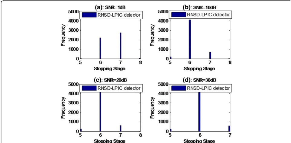
In Figures 7, 8, and 9, the sensitivity of the L-curve method with respect to the condition number of the sys-tem matrix (which varies with the time varying fading channel) is evaluated for different SNRs. The same param-eters used in Figures 5 and 6 are used here as well except for the SNRs where the SNR is fixed to 1, 10, 20, and 30 dB, respectively. In addition, the L-curve technique is used over 5,000 consecutive OFDM symbols and the histogram of the stage indices of the RNSD-LPIC and
CGLS-LPIC detectors are plotted in Figures 8 and 9, respectively.
As depicted in Figure 7, the condition number of the system matrix varies from one OFDM symbol to another and it is dependent on the fading channels of the differ-ent users. It can be seen that the condition number of the system matrix varies largely in magnitude where it can go from 103to 106.
As depicted in Figures 8 and 9, it is clear that the stop-ping stage determined by the L-curve method for both the RNSD-LPIC and CGLS-LPIC detectors is almost fixed with respect to the condition number variations of the sys-tem matrix over 5,000 OFDM symbol (see Figure 7) for
each SNR. Consequently, it is sufficient to evaluate the stopping stage index for a few OFDM symbols (say 100 OFDM symbol) and then get the average stopping stage index and use it for the subsequent OFDM symbols. This is a very important result as it allows avoiding the calcula-tion of the stopping stage for every OFDM symbol and thus renders this scheme very efficient in terms of compu-tational complexity.
It also is clear that the stopping stage is almost constant on average with increasing SNR while in principle, it should increase. This is one of the deficiencies of the L-curve method, and it is due to the fact that the L-L-curve method is not a converging stopping rule, in the sense that
Figure 6The (a) residual's norm and (b) its curvature of the CGLS-LPIC detector.
the solution obtained using the L-curve method does not converge to the true solution if the noise variance vanishes to zero.
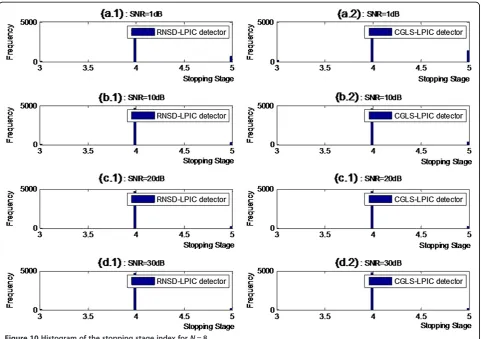
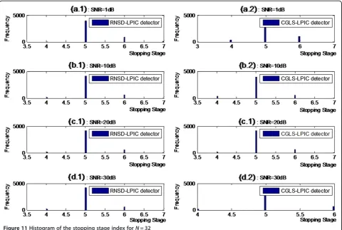
The L-curve method is somewhat sensitive to the size of the system matrix determined by the number of subcar-riersN. To illustrate this fact, we plot the histogram of the stage indices determined by the L-curve method over 5,000 OFDM symbols for two values of the subcarriersN,
that is N= 8 and N= 32, respectively. We can see from Figures 10 and 11 that the most dominant stage index for N= 8 is four stages while the most dominant stage index for N= 32 is five stages. In addition, we have seen previ-ously from Figures 8 and 9 that for N= 128, the most dominant stage index is six stages which indicates that the most dominant stage index increases with the number of subcarriersN.
Figure 8Histogram of the stopping stage index for SNR = (a) 1 dB, (b) 10 dB, (c) 20 dB, and (d) 30 dB.
This suggests that the stopping stage determined using the L-curve method should be updated whenever the total number of subcarriersNin the system changes, for example, if one user needs a higher data rate and is assigned a higher number of subcarriers, or if one user enters or leaves the system, etc.
In Figure 12, we evaluate the convergence behavior of both the RNSD-LPIC and the CGLS-LPIC detectors equipped by the L-curve stopping rule by varying the stage indexpand assessing its average BER performance. For comparison purposes, we simulate also the decorre-lator (DEC) and the LMMSE (LMMSE) detectors. We use the same simulation parameters as in Figures 5 and 6 but we set the SNR to 13 dB. One can see the semi-convergence behavior of both the RNSD-LPIC and the CGLS-LPIC detectors and how the detectors equipped with the L-curve method stop at six or seven stages and yield an average BER that is between that of the decorr-elator and LMMSE detectors yet they do not require any information about the noise variance.
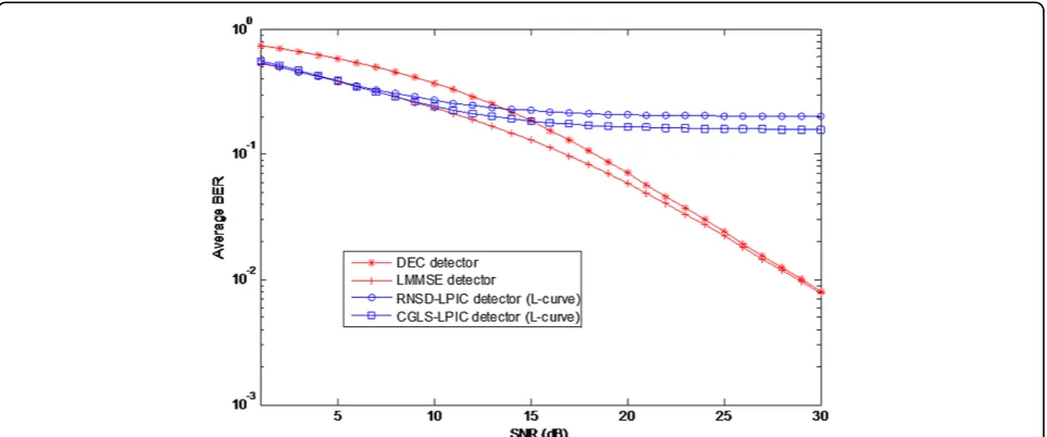
Figure 13 illustrates the average BER performance versus the SNR of the RNSD-LPIC and the CGLS-LPIC detectors equipped by the L-curve stopping rule. It is clear that the RNSD-LPIC detector performs better
than the decorrelator detector if the SNR is less than 15 dB and the CGLS-LPIC detector performs better than the decorrelator detector if the SNR is less than 16 dB. This suggests that the L-curve method can be used only for low to medium SNRs; fortunately, these regions suffer the most from the noise enhancement effect, and therefore, this deficiency of the L-curve method is not serious.
8. Conclusion
In this work, we introduced new linear interference cancellation detectors for low to medium SNR ill-conditioned communication systems that perform close to the LMMSE detector though they do not require the knowledge of the noise variance information. These lin-ear IC detectors are based on lin-early an stopping rule known as the L-curve method. Simulation results indi-cate that these detectors are insensitive to both the con-dition number of the system matrix and SNR and can work well up to SNR of 16 dB.
Appendix
In the following, we develop the average BER of the RNSD-LPIC and CGLS-LPIC detectors.
The QPSK scheme can be seen as two superimposed BPSK channels, these channels are orthogonal to each other and do not mutually interfere; therefore, the BER of QPSK scheme is simply the same as that of the BPSK scheme, and it is enough to conduct the BER probability
analysis using the real or imaginary part only. In this derivation, we consider the real part of the decision vectoryp.
The vectors yp and b can be decomposed as yp=
[yp,1yp,2⋯ ⋯yp,n⋯yp,N]Tandb= [b1b2⋯ ⋯bn⋯bN]T;
therefore, the real part of thenth element of the vectoryp can be written as:
ℜ yp;n
wherenis a vector of AWGN I.I.D samples of zero mean and varianceρ2. By using the total probability theorem, we can write.
Due to the symmetry of the Gaussian (Normal) func-tion, we have
thus
Conditioning over all interfering bits, the probability of error can be written as:
Pbðp;nÞ ¼
Averaging over all subcarriers, we obtain
Pbð Þ ¼p
cflop states for any complex addition, complex sub-traction, complex multiplication, or complex division.
Competing interests
The authors declare that they have no competing interests.
Author details 1
Prince Sultan Advanced Technologies Research Institute (PSATRI), King Saud University, P.O. Box 800, Riyadh 11421, Saudi Arabia.2KACST-Technology
Innovation Center in Radio Frequency and Photonics for e-Society (RFTONICS), Electrical Engineering Department, King Saud University, P.O. Box 800, Riyadh 11421, Saudi Arabia.
Received: 9 March 2013 Accepted: 19 November 2013 Published: 5 December 2013
References
1. ML Honig,Advances in multiuser detection(Wiley Series in Telecommunications and Signal Processing, Hoboken, NJ, 2009) 2. Z Peng, Z Xu, W Furong, X Xu, T Lai, A relay assignment algorithm with
interference mitigation for cooperative communication, in WCNC. Budapest
5–8, 1286–1291 (2009)
3. SW Hou, CC Ko, Intercarrier interference suppression for OFDMA uplink in time- and frequency-selective fading channels. IEEE. Tran. Vehicular. Technol.
58(6), 2741–2754 (2009)
4. M Takanashi, T Nishimura, Y Ogawa, T Ohgane, MIMO-UWB systems with parallel interference canceller using timing control scheme in LOS
environments. inIEEE. Wireless. Commun. Netw. Conf. (2007), Kowloon, 11–15 March 2007, pp: 1599–1603
5. H Mrabet, I Dayoub, R Attia, S Haxha, Performance improving of OCDMA system using 2-D optical codes with optical SIC receiver. J. Lightwave. Technol.27(21), 4744–4753 (2009)
6. E Axell, EG Larsson, Optimal and sub-optimal spectrum sensing of OFDM signals in known and unknown noise variance. IEEE. J. Select. Areas. Commun.29(2), 290–304 (2011)
7. EG Larsson, R Thobaben, G Wang, On diversity combining with unknown channel state information and unknown noise variance. inProc. of IEEE Wireless Communications and Networking Conference (WCNC), Sydney, 18–21 April 2010
8. B Abdelouahab, SA Alshebeili, Regularization property of linear interference cancellation detectors. EURASIP. J. Adv. Signal. Proc.2012, 145 (2012) 9. U Hamarik, R Palm, On rules for stopping the conjugate gradient type
methods in ill-posed problems. Math. Model. Anal.12(1), 61–70 (2007) 10. IEEE Standard for Local and Metropolitan area networks Part 16, Air interface
for fixed and mobile broadband wireless access systems amendment 2: physical and medium access control layers for combined fixed and mobile operation in licensed bands, 802nd edn(The Institute of Electrical and Electronics Engineering, Inc. Std. IEEE, Piscataway, NJ, 2006) 11. SK Hashemizadeh, H Saeedi-Sourck, MJ Omid, Sensitivity analysis of
interleaved OFDMA system uplink to carrier frequency offset, in2011 IEEE 22nd International Symposium on Personal Indoor and Mobile Radio Communications(, Toronto, ON, 2011), pp. 1631–1635
12. NM Thamban,Linear operator equations: approximation and regularization (World. Sci. Publ. Co., Singapore, 2009)
13. C Hansen,Rank-deficient and discrete ill-posed problems: numerical aspects of linear inversion(Society for Industrial and Applied Mathematics, Philadelphia, PA, 1998), pp. 403–6
14. J Nagy, K Palmer, Steepest descent, CG and iterative regularization of ill-posed problems. BIT43, 1003–1017 (2003)
15. PC Hansen, The L-curve and its use in the numerical treatment of inverse problems. Comput. Inverse. Prob. Electrocard.2, 1–24 (2000)
16. PC Hansen, TK Jensen, G Rodriguez, An adaptive pruning algorithm for the discrete L-curve criterion. J. Comput. Appl. Math.198(2), 483–492 (2006) 17. P Qu, K Zhong, B Zhang, J Wang, GX Shen, Convergence behavior of
iterative SENSE reconstruction with non-Cartesian trajectories. Magn. Reson. Med.54(4), 1040–5 (2005)
18. DR Joshi, DC Popescu, OA Dobre, Adaptive spectrum sensing with noise variance estimation for dynamic cognitive radio systems, inCISS 2010(, Princeton, NJ, 2010), pp. 1–5
19. GH Golub, CF Van Loan,Matrix computations, 4th edn. (The Johns Hopkins University Press, Baltimore, MD, 2013)
doi:10.1186/1687-6180-2013-180
Cite this article as:Bentrcia and Alshebeili:Linear IC detectors for low to medium SNR ill-conditioned communication systems with unknown noise variance.EURASIP Journal on Advances in Signal Processing 20132013:180.
Submit your manuscript to a
journal and benefi t from:
7Convenient online submission
7Rigorous peer review
7Immediate publication on acceptance
7Open access: articles freely available online 7High visibility within the fi eld
7Retaining the copyright to your article