Drift correction using a multi rate extended Kalman filter

(1)

Drift correction using a multi-rate

extended Kalman filter

(2)

Abbreviations

HMD – head mounted display. XME – Xsense MVN engine. OPS – optical positioning system.

Pose – orientation and translation. (typically represented by a 4x4 matrix in this document) KF – Kalman Filter.

RMS – Root mean square.

Abstract

This work proposes an algorithm to improve an existing positioning system in a virtual reality application. This existing system uses the inertial based XME (Xsense MVN engine) which is prone to drift. Drift is a real problem, because accidents can happen when the virtual world is misaligned with the designated play area in the real world. After considering several approaches we settled on using a second positioning system in the form of an optical inside-out approach. In order to deal with the opportunistic and desynchronised nature of this method we developed a multi-rate

extended Kalman filter for the sensor fusion. The filter was designed with two update steps, one for each positioning system. One update step takes the pose of the OPS and the other a delta pose of the current and previous XME pose. With this approach a test was done where the designed OPS error model and the delta approach were compared to simple alternatives. The test used a third, proven, pose estimation system (the optitrack) to provide ground truth poses. The results show that the OPS error model doesn't improve much over a static error. The delta approach is very preferable

(3)

1 Introduction:

Within a virtual reality simulation a user has limited awareness of his/her surroundings. This makes it important that the system accurately aligns the virtual world with the real world. If they do not align, a user may walk into obstacles (for example walls or other players) in the real environment while avoiding them in the virtual one. Besides in augmented reality and virtual reality pose estimation is also an important aspect in robotic navigation.

RE-liON works on a multi user virtual reality simulator. The application is meant to provide realistic virtual training scenarios for several fields of crisis management. Small teams are able to partake in a virtual scenario together. Because the environments in these scenarios are virtual, the same physical environment can be used for many different scenarios. The setup of the system itself is mobile, meaning that it is relatively simple to move the setup to an other location if required. This simulator is used as the target application for this research.

For pose estimation RE-liON currently uses a full body wearable motion capture suit (from Xsense https://www.xsens.com/ ) that possesses a series of inertial measurement units that track the user's relative movements limb from limb. With the Xsense MVN Engine (XME) poses (translation and orientation) are generated for a range of body parts by fusing magnetometer measurements together with the IMU measurements. The poses are generated at a high frequency with small relative error, but the XME suffers from drift (accumulated error) when it is used for longer periods of time. Besides drift sudden distortions can also happen. Because XME works relative to itself, it is not able to recover without additional data.

A second pose estimator is used to tackle the problem of drift. The estimations of both systems can be combined to create a more robust and accurate system. The second estimator should provide data that enables the positioning system to recover from drift and other possible errors. This means that the second pose estimator mainly serves as a correction for the XME positioning system. Optical positioning systems (OPS), which are discussed in detail in section 2, fulfil the requirements of being portable and lightweight, as well as robust, accurate and free of drift. For those reasons we chose to use an OPS in this work.

The extra data the OPS offers is fused together with the XME data in an effort to increase the robustness of the positioning system. A popular technique for sensor fusion is the Kalman Filter. A few challenges arise fusing the systems together when using the Kalman filter. Both positioning systems work individually, in separation of each other. In this case that means that both systems work in different coordinate systems. Furthermore the timing and frequency of the OPS depends on whether markers are detected in a frame. Not only is the frame rate of the camera different from that of the XME system. The OPS provides intermittent measurements which depends on the actual circumstances and cannot be predicted. In this work we address both these problems.

Another challenge we encountered is that the error on the OPS measurements are not normally distributed. Kalman filters are predicated on the assumption that both observation noise and system noise are normally distributed. As we will discuss in section 3.2.2, not only is the observation noise of the OPS not normally distributed, its statistics depend on the measurement. We leverage these properties of the noise to make the fusion more accurate.

This leads us to the following main question:

• Does the proposed model correct the drift and thus increase the accuracy over time compared to the XME?

(5)

• How do we tackle the misalignment of the positioning systems?

• How do we fuse together two positioning systems with different rates, where one also has inconsistent timing?

• How to deal with measurement dependent noise?

A model has been developed using the extended Kalman filter to tackle these challenges. The model makes use of two different update steps, one for each of the pose estimators. This was done to circumvent the challenge of timing and frequency differences. To tackle the varying misalignment, which grows as the XME accumulates drift, between the two coordinate systems we used the difference between the latest and second latest poses of the XME system. Because of this we refer to the model as the delta model throughout the document. We also propose a noise model for the OPS measurements that depends on the size of the marker by counting the amount of pixels.

2 Optical positioning

In this chapter several design options are explored. We start with the cameras' placement, mounted on the users or around the tracking area. Then we look at what method of tracking we will use. After we decided to use markers we explored some different marker options.

2.1 Literature Review

2.1.1 Inside-out or Outside-in

For optical solutions in tracking a person's location there are two approaches. You can either use inside-out tracking or outside-in tracking.

Outside-in

[image:5.595.272.536.456.633.2]

An optical outside-in solution would be where one or more cameras are placed so they would cover the whole playing field. Users can be identified and their positions can be calculated as long as they are in the view of one or more cameras. Markers can be used to make the identification or pose estimation easier and more accurate. Markers would serve as an indication of the the actual point that is supposed to be tracked.

Figure 1: Outside-in tracking using three optical sensors. The user can be equipped with markers for tracking or identification.

Cam 1

Cam 2

Cam 3

(6)

Inside-out

A solution for inside out optical pose estimation is when one or more cameras are mounted on the user(s). Images of the natural features in the environment or markers placed in the

environment allow the position of the user to be estimated. Kiyoung et al [KMYWJ05] present a game that uses an inside-out approach where the markers are placed on the ceiling while a camera facing upwards is mounted on the users' head.

Both options are realisable in the target application. So they are compared to each other to decide which one seems most suitable.

• Tracking area:

◦ For the outside-in approach the tracking area is as big as the area the cameras can cover but are still able to correctly track the users. Depending on the how the cameras are placed in the environment, it might be difficult to cover larger areas. For example: If the cameras are mounted on a support on the side line of the area, the middle of the field might not be covered depending on the range of the cameras. For inside-out tracking the area size depends on the method used. If natural features are used the area is

theoretically limitless. If a system that relies on markers is used, the size is limited to the area where the markers are placed.

• Cameras used:

◦ For outside-in the number of cameras required depends on the area that needs to be covered as well as the range of the cameras. If one camera covers the whole area, one can be sufficient. Using more than required could result in an increase of the robustness and/or accuracy. For inside-out at least one camera per user is needed. In this case multiple cameras can also be used to increase the robustness and/or accuracy. Also different types of cameras can be explored. For example stereo cameras or cameras that are capable of measuring depth. Although such camera offer limited benefits with marker-based systems, they can be beneficial when natural features are being tracked.

• Camera failure:

◦ When camera failure occurs using an outside-in approach the tracking area decreases (unless it has complete overlap with other cameras). During camera failure in an inside-out the user will not be able to receive any optical pose estimations any more, but it should have minimal effect on the other users.

• Setup:

[image:6.595.58.362.69.239.2]

◦ In the inside-out configuration the cameras are likely to be mounted on the equipment users are wearing. For outside-in the camera(s) need to be distributed in and/or around the designated area. Also the power supply need to be addressed here. Although outside-in cameras can use wired power provision ans outside-inside-out cameras require portable battery-provided power, in the current setup inside-out cameras can be connected to the Figure 2: Inside-out tracking. A camera mounted on the head

mounted display allows for pose estimation of the person's head. (image source:

(7)

mobile computer which is already present. The downside is that it will demand some of the limited onboard processing power and memory. For outside-in each camera needs to be connected to the server of the application.

• Occlusion:

◦ Because the users already possess the XME pose estimations, occlusions aren't a big problem in this application. For either approaches, if occlusion occurs or not, the positions are continuously estimated by XME. Although the longer a user is tracked solely on the XME measurements, the more drift can be expected.

The inside-out application is chosen as more favourable mainly because of the setup. That setup enables an easy accessible power supply for the camera. The tracking area is also more easily defined and markers are generally easier to install around the area than cameras are. Also this way there is no identification process needed for the user.

2.1.2 Optical positioning feature based or using Fiducial markers

Visual odometry is known as the process of estimating the change in position over time through the use of subsequent images. Through the use of optical flow in the images relative motion can be estimated. Visual odometry includes lots of techniques popular in robot localization. The basic structure of a visual odometry procedure is as follows:

1. The acquisition of image(s).

2. Correction the image of possible camera distortions.

3. Detecting features and correlate them to the previous frame(s). 4. Outlier filter.

5. Motion estimation.

6. Repopulation/ key-frame update (if necessary).

C. Forster et al [CMD14] present a open source implementation of their semi direct visual odometry approach. In their approach they eliminate the need for feature extraction by operation on pixel intensities directly. They claim it provides increased robustness in little, repetitive, and high frequency-texture envorinments compaired to traditional solutions.

Extensions to visual odometry are SLAM (Simultaneous localization and mapping) and PTAM (Parallel tracking and mapping) [JTD14]. SLAM and PTAM use visual odometry techniques to calculate the relative motion but at the same time also maps the environment simultaneously (or parallel). The additional information the map provides can then be used to help with the drift. The map also helps the system to be able to recover fast when it loses track of its pose, for example when movement between two frames is large enough that little to no features of the previous frame are visible in the new frame. If the new frame does contain features which are already mapped before, it should be able to recover relatively fast. It should be noted that during the map generation drift is still present.

(8)

consists of the following steps:

1. The acquisition of image(s).

2. Correction the image of possible camera distortions. 3. Detecting potential markers.

4. Outlier filter.

5. Marker identification 6. Pose estimation.

In [SILT12] section 4.4.1 they give general guidelines about when to use marker based tracking in favour of feature tracking. Some of the cases that might apply to the target application:

• Challenging static environments for feature tracking.

◦ In these environments feature tracking can become very unreliable, for example an environment with a low amount of traceable feature. Another example is environments with repetitive textures. Here feature tracking solutions can become confused due to the large number of similar features. It is possible to alter the environment by adding additional features to track, but in that case it loses an advantage it has over using fiducial markers.

• Non static environments.

◦ When the background of the environment contains (a lot of) moving objects or persons it might confuse a feature based tracking system as features can constantly change. For example an environment with trees. Trees can already be considered to have repetitive texture but the features also vary in position as soon as a the wind blows through the leaves.

• Occlusion

◦ When the background often gets occluded by moving objects or persons a feature-based tracking system can lose track. When the camera is no longer occluded it is possible for such a system to recover, but this gets harder if the camera's pose changes during the occlusion. Then the there could be little to no familiar features left to figure out the current pose.

• Convenient coordinate frame.

◦ Without some additional and/or initial information a feature based tracking system will not be able to deduce earth coordinates or scale. A marker-based system will easily be able to deduce those as they are provided the necessary information in the marker dimensions.

• Efficiency

◦ Typically, marker-based systems are easier to implement. So if tracking is not the focus of a project it is generally faster to get to a proof of concept using a marker-based system.

• Limited computational capacity

◦ Generally marker-based systems are less demanding with processing power and memory.

(9)

2.1.3 Feature and marker Hybrid systems

A hybrid system will be able to use the versatility of the feature-based system with additional information from markers. The markers can be used as a means to correct potential drift in the feature based system and serve as a good initialisation point for getting the right scale and coordinate space.

This option is not chosen because the XME pose estimation already has similar results to a feature-based solution. They both support high relative changes but suffer from a drift. The XME system is currently a vital part of the system. Next to pose estimation it is also used for estimating a person's stance.

2.1.4 Marker type

When using predetermined markers there are several option to choose from.

Active / passive markers

The choice is between active and passive markers. Active markers are markers which actively send a signal, an optical application for this is the usage of lights as markers. Often infra red lights are used, as these are invisible for the human eye but visible with a camera with an infrared filter. Although one should be careful using this in

environments with a lot of infrared light from the environment (for example outside in sunlight). A similar option can be used with passive markers. In that case the camera will be equipped with the infra red lights, and the markers used are retro reflective. A retro reflective marker reflects light back to the source with a minimum of scattering. More popular is a passive black and white marker, which can simply be printed on a piece of paper.

Shape

The research in [STOR12] showed that the most popular are square and circle shaped markers. Both can be used for pose estimation, but prior work

indicates that that using circles has a higher pose estimation accuracy and is more robust to noise and perspective distortion [AJD11a]. Square markers on the other hand have a larger data capacity. Square markers are still chosen instead of circle markers because of the accessibility/ license of the available libraries.

Identification:

To be able to use multiple markers the markers have to be distinguishable. In [SILT12] they mention three types:

• Template markers: each marker has its own template, when a marker is detected. Its template will be matched with the template database to see which template it most resembles.

[image:9.595.333.516.360.510.2]

• Barcode markers: These often have a binary data grid in which can be converted to a identification number. They can also make use of error correction. A. Rice et al [ACJ05] presents a scheme that makes efficient use of the available payload while still providing a large degree of error correction which they claim requires the minimal amount of computer vision.

(10)

• Imperceptible markers: Markers that are not immediately recognised as markers, for example the use of images or miniatures.

Size and colour

Bigger is better for pose estimation as the shape of the marker is described in more pixel (when looking from the same distance) and they will be better recognised from a longer range. But they also are easier occluded or partially out of frame. Black and white offers the highest contrast, but colours might enable easier recognition of the marker by colour filtering.

Position (vertical/ horizontal)

For this work we place the markers on the ground rather than placing them on walls. There are more options available for placement density when placing the markers on the ground. There can also be a guaranteed distance to one or more markers for the users in that case. If desired both options can be easily used together. For the thesis only ground markers are used. These markers are assumed to have a height of 0.

2.2 Marker detection and pose estimation

To make optical pose estimations the ArUco library is used (presented by S. Garrido-Jurado et al [SRFM14]). The library is easy to implement and is available for use under a BSD license. They show the results are comparable with other AR libraries (for example: ARTag [FIAL05] and ARToolKit [DD07]) which also offer pose estimation with AR-markers. They claim to have better results in terms of false positive rate.

The ArUco library uses contour based algorithm to find the markers. After getting an image as input the library uses the following steps to make a pose estimation:

1. An adaptive threshold on the greyscale image to get a binary image. An adaptive threshold thresholds around the relative local contrast. The adaptive threshold is preferred over a normal threshold to deal with unequal lighting. It also immediately serves for line detection. 2. Rectangle detection: The contours of each blob in the image is extracted. After a polygonal

approximation is performed. Blobs that are not approximated to 4-vertex polygons are discarded. Several other checks are implemented as well (to thin out the number of potential markers).

3. Identification. The remaining potential candidates will enter the identification process. After a perspective projection of the candidate, it is divided in a binary data grid. The 4 different rotations of the grid are then checked to see if one of them belongs in the marker dictionary. If none of the rotations belong in the dictionary a correction method is available. A. Pagani et al [AJD11b] described several design options in their section about marker identification. ArUco uses the so called Code Bins (subdivision in binary bins) which is the most

commonly used method.

4. Pose estimation. First corner refinement is applied by applying linear regression to the marker side pixels to calculate their intersection. The corners are then used for pose estimation by iteratively minimizing the re-projection error of the corners.

Optical sensor:

(11)

well enough up to a distance of 3 meters. A higher resolution should increase the range and accuracy of the pose estimation (as there will be more pixels describing the marker). Although a higher resolution will also increase the computation time of the marker detection.

Camera calibration

To preform accurate optical pose estimation, the camera's intrinsic calibration should be known. To find the intrinsic parameters a popular camera calibration method is used. The OpenCV library has the necessary methods to calculate the intrinsic parameters as well as some distortion coefficients. The parameters can be saved and reused for the camera. This process should be done for each individual camera.

Hand-eye calibration

The position delivered by the XME corresponds to a point that falls within the user's head. It is not entirely clear where this position is in relation to the IMU sensors. The position of the optical sensor is on top of a user's helmet on the front. The relative position of these positions is supposed to remain constant and thus is considered rigid.

Because the optical pose estimator estimates the position of the camera, the relation between the that position and the XME position should be known. If not, the XME will be corrected to the camera position and as the camera position is actually several centimetres in front of the XME position errors are introduced. These errors are especially noticeable when a user rotates. Then both the OPS and XME both measure an different translation (see Figure 4).

A proper way to estimate the relation is to use a existing hand-eye calibration technique. But for this work hand measurements were taken with measurement tape. These measurements are expected to contain a small error. An existing algorithm was not used to save time as it falls outside of the scope of the project.

3 Sensor fusion

In this chapter the fusion algorithm that is used in this project is explained. First a short explanation for the algorithm we want to use, the Kalman filter. Then we look at what information the

[image:11.595.307.537.316.441.2]

positioning systems give us, followed by how we use that information to form a model for the filter. Because the model can't be used by the standard Kalman filter we then explain how it is used with the Extended Kalman filter.

Figure 4: When a user rotates him/ her-self on the pivot point of the XME head position, the XME will not perceive a change in the position. However, as the camera is not positioned on that pivot point the optical sensor will measure a translation (assuming the optical sensor is able to estimate its pose in both poses). In the image the green dot represents the XME head position and the camera is positioned on the front on top of the user and is coloured red.

Yaw: 0 XME: (0,0) OPS: (0,2)

(12)

3.1 Kalman Filter

A popular technique used for sensor fusion is the Kalman filter [KALM]. The Kalman filter consists of two parts, the prediction step and the correction step. The Filter first predicts the next state based on the previous estimate and the state transition model in (1) and also predicts the corresponding covariance with added noise in (2) in the prediction step. Then, in the correction step, a Kalman gain is calculated based on the relative certainty of the measurements and the current state

prediction (3). The Kalman gain is a relative weight for the measurements and current prediction. Using the Kalman gain and the measurements, the predicted state is updated to get the corrected state in (4). Then the corresponding covariance is calculated using the same Kalman gain (5). (The control vector is omitted as no control input is included).

Prediction:

̄

X_k=F X̂_k−₁ (1)

̄

Pk=FP̂k−1F

T

+Qk (2)

Estimate:

Kk= ̄PkHT(H P̄kHT+Rk)−1 (3)

̂

X_k= ̄X_k+K_k(M_k−H X̄_k) (4)

̂

P_k=(I−K_kH) ̄P_k (5)

Where:

F = Transition matrix H = Observation matrix I = Identity matrix ̄

X = Predicted state ̂

X = Estimated state ̄

P = Predicted Covariance ̂

P = Estimated Covariance

M = Measurements / Observations Q = Process noise

R = Measurement noise K = Kalman gain

(6)

3.2 Available data

First we look at the information that is provided by the positioning systems. Using this information a model is created. The XME delivers a series of poses containing an estimated translation and orientation of several body parts of a user. A pose is constructed as follows:

Pose=

[

R₁₁ R₁₂ R₁₃ 0 R₂₁ R₂₂ R₂₃ 0 R₃₁ R₃₂ R₃₃ 0 Tx Ty Tz 1

]

(7)

(13)

The poses are not directly measured. XME instead uses accelerometers and gyroscopes together with magnetometers to calculate the poses. Furthermore, the poses delivered are not the poses of the sensors themselves, but rather of bones of body parts nearby the sensors. These poses will be called XME poses in this document.

Only the pose of the head is used for fusion. The head is chosen because the position and

orientation of a user's head are crucial when it comes to virtual reality as the eyes are located there. The VR world is therefore rendered with respect to the head's pose. The helmets users wear are also an easy location to mount a camera and this way the camera's images can also be used for other applications, for example to give a user vision of what is ahead of him/her (if needed) without removing the HMD. (In addition, in the current application, users typically carry a weapon. If the weapon is inside the camera's field of view, it can also be used to improve the weapon's pose estimation.)

The OPS delivers a pose estimation with a similar structure as the pose in (7). This pose is the translation and orientation of the camera. It is estimated relative to the marker found in an image. If no marker is detected in a particular frame, the OPS doesn't deliver a pose.

Both systems deliver a similar output pose estimation of the same pose. So when using them

together they can be considered as competitive. The only problem with this is that they both work in a different coordinate system. The XME pose is estimated as a relative rotation and translation to its initialisation position. This initial position is reset every time a XME calibration is performed. The XME calibration matches a person's body pose to the virtual character pose. In contrast, the OPS pose is estimated relative to the marker(s). The system should possess the layout (the position and rotation) of each participating marker. Without the position and orientation of the markers in world space the OPS can only estimate its pose in relation to the marker.

3.2.1 Model

To be able to use the Kalman filter, a model is needed. The variables modelled together with their transition need to be specified. It is also required to specify how the observations contribute to the state. The state vector used is shown in (8). The state vector consists of the following:

• X and Z position together with a yaw of the forward vector (in a coordinate system where Y is perpendicular to the ground). These are the values that we want to estimate for the

positioning system. The pitch and roll are not included in the filter as XME itself delivers adequate measurements without drift using the accelerometer (which makes use of the gravity). The Y position (the height) is also excluded as the XME value is deemed adequate. (thus only simplifying the model by excluding them)

• The Delta ( differences between Statek and Statek−1 ) values of the X and Z translation and the Yaw rotation. These are the changes between the latest two iterations.

(14)

State vector=

[

Position_x Position_z Yaw

ΔPosition_x ΔPositionz

ΔYaw

Movement speed Movement direction Yaw rotation speed

]

(8)

When transitioning to the next state State_k the formulas in (9) are used for the prediction step. Where Δt is the time between State_k and State_k−₁ .

xposk = xposk−1+speedk−1Δtsin(directionk−1) zpos_k = zpos_k−₁+speed_k−₁Δtcos(direction_k−₁)

yawk = yawk−1+yawSpeedk−1Δt Δxpos_k = speed_k−₁Δtsin(direction_k−₁) Δzposk = speedk−1Δtcos(directionk−1)

Δyaw_k = yawSpeed_k−₁Δt speedk = speedk−1

direction_k = direction_k−₁ yawSpeed_k = yawSpeed_k−₁

(9)

Although the XME delivers a pose, the pose will not be directly used in the filter. The reason for this is that the position the XME delivers is relative to its initial position. The position is basically a summation of all the movements made since the initialisation. The measurements XME uses for its pose are accurate but still have a small error. This means that the summation will also include the sum of all the errors which results in a drift which means that the position that is delivered will become less accurate over time. If the position with increasing variance is used as a direct

measurement, it will result that the XME observations will contribute less and less to the estimation (this is visible in the results where the delta model is compared to a position model). At some point this causes the filter to almost solely estimate the position on the prediction (and optional OPS observations). As the predictions alone can't deliver accurate estimations over longer periods of time, this approach isn't a viable option. So instead the difference between two XME measurements are used, the deltas (10). The error between two XME measurements does not keep increasing over time (Figure 5). The individual error between two pose measurements can still differ depending on the time between measurements.

XME Measurements=

[

ΔPosition_x ΔPosition_z

ΔYaw

]

(15)

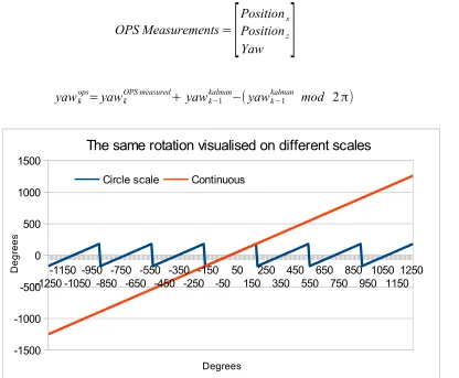
The OPS measurements also deliver a pose. The X and Z measurements are used directly, only the yaw isn't used directly. The yaw will be the result of (12). This is done to synchronise the number of complete rotations an user has done with the current OPS observation, as the rotation used in the filter is a continuous summation of the deltas. The reason for this is to keep the yaw representation linear for the filter (Figure 6). Additionally, 2π will be added or subtracted if the difference between yawk

ops

−yawk−1

kalman

is still above π _{or below} −π _{. This is done to ensure the}

smallest rotation is used. No deltas are calculated for the OPS observation because they are assumed to be available very inconsistently.

OPS Measurements=

[

Position_x Position_z Yaw

]

(11) yawk ops

=yawk

OPS measured

+ yawk−1

kalman

−(yawk−1

kalman

[image:15.595.37.564.46.256.2]

mod 2π) (12)

Figure 5: Illustrative noise representations for consecutive steps. The X means that there are is no observation available. The bigger the size of the circle, the higher the noise variance.

t0 t1 t2 t3 t4 t5 t6 t7 t8

XME pose

OPS

_X

XME

_X

Figure 6: difference in scale for yaw. The continuous one is used for our model.

-1250 -1150 -1050 -950 -850 -750 -650 -550 -450 -350 -250 -150 -50 50 150 250 350 450 550 650 750 850 950 1050 1150 1250 -1500 -1000 -500 0 500 1000 1500

The same rotation visualised on different scales

Circle scale Continuous

[image:15.595.85.501.433.776.2]

(16)

3.2.2 Noise estimation

During preliminary testing of the pose estimation we noticed that the error on the OPS measurements wasn't normally (Gaussian) distributed. In particular, that the error on the OPS measurement correlates with the size of the marker in the camera image. This latter size is available when the detection is done, so that we can estimate the noise on the measurement as a function of the marker's size. In this section we develop this idea and describe how we parametrise the OPS measurement noise.

[image:16.595.341.536.86.267.2]

To get a rough estimation of error that is measured, multiple measurements in a grid shape have been made (Figure 7). It was a 7 by 7 meter grid with the marker position in the centre of the grid, resulting in a

maximum X and Z distance of 3 meter (with maximum distance in the corners being

_√

32+32 ). The marker in the middle has dimensions of 29.5 x 29.5

centimetres. The positions in the grid were measured by hand with the help of spring rulers.

On each of the 48 positions (no measurements were taken on position 0,0) 5 series of 30 frames were taken with 5 different yaw angles. The angles don't follow a predefined value. Instead they are decided by the position of the marker in the camera image. This is done to ensure that there are always 5 measurements with different angels as the angle at which the marker is visible changes with the distance to the marker.

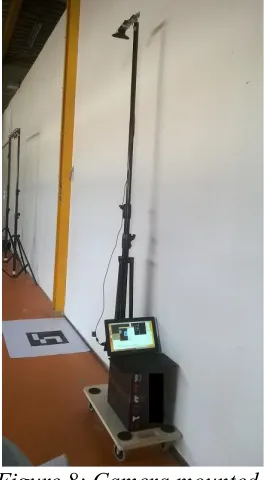
For this test a camera (the Logitech HD Pro webcam 910) was mounted on top of a pole which in turn was mounted on a mobile cart (Figure 8). The height of the camera in this setup is 1.80 meters. The camera was connected to a mobile computer running the pose estimation software. A pivot point directly underneath the camera was used to rotate around for the different angles.

The pose estimation software calculates a pose for each frame in which the marker is identified. If the marker is successfully

identified in all frames it would total to 7200 poses. These estimates are then checked on how much they differ from the measured positions.

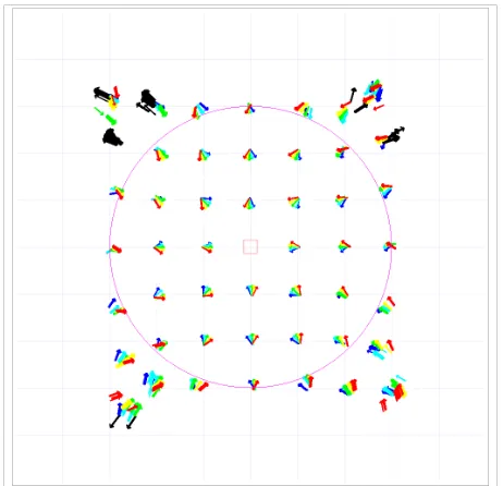
[image:16.595.61.193.479.719.2]

An overview of the estimations is presented in Figure 9. Each measurement position consist of collections of arrows. The colour coding of the arrows (except black) corresponds with the marker position in the image (far left, left, middle, right and far right). The black arrows are cases where the estimation presumes a wrong perspective (Figure 11). These cases are discarded. The magenta circle in the images represents the 3 meter distance to the marker.

Figure 7: Measurement positions in grid formation. The orange square is the marker position and the blue tilted squared are the positions where measurements were taken.

-4 -3 -2 -1 0 1 2 3 4

-4 -3 -2 -1 0 1 2 3 4 measurement positions

X in meters

Z in m e te rs

(17)

Each of the remaining poses is compared to the measured value. The distances between the measured and estimated position are regarded as errors. Figure 10 shows the same error but then against the area of the marker in pixels.

A function of the trend-line of the error against the marker area is calculated for use in the sensor fusion. It is recommended to recalculate the function when using different camera settings because different settings might give different results, especially if the resolution is different.

There were no recorded instances where the marker was identified with a wrong id. There were also no recorded instances in false positives (finding a marker where there is no marker)

[image:17.595.310.541.81.304.2]

The value used for OPS observation noise is calculated based on the area of the marker found in the image instead of the distance because the distance is estimated and the area is measured. The Yaw currently has no estimated noise value. The same counts for the observation noise for XME measurements and for process noise. The values for those is set by a trial and error approach.

Figure 9: Estimated positions and directions of the camera pose for the grid test. The black arrows are estimations which took a wrong perspective and are discarded. The rest of the colour coding represents the roughly where the marker was positioned in the image (far left, left, middle, right, far right).

Figure 10: The error between measured and estimated positions. The trendline is used for error estimation for OPS

measurements.

0 0.1 0.2 0.3 0.4 0.5 0.6 0.7 0.8

f(x) = 174.11 x^-0.93

Estimation error against the marker area

Pixels

e

rr

o

r

in

m

e

te

[image:17.595.134.449.506.692.2]

(18)

3.2.3 Extended Kalman Filter

The state transition includes non linear formulas and because the regular Kalman filter requires the model to be linear, the Extended Kalman filter is used instead. The Extended Kalman filter is very similar to the Kalman filter but has added linearisation of the state transition model and the

measurement model. Formulas (13) to (17) are of the extended Kalman filter, where only (13) and (16) have a small change compared to the regular Kalman filter. An other difference is that F and H are now Jacobian matrices of f(X) and h(X) which have to be recalculated every iteration.

Prediction step:

̄

X_k=f( ̂X_k−₁) (13)

̄

Pk=FkP̂k−1FTk+Qk (14)

Estimation step:

Kk= ̄PkHT(H P̄kHT+Rk)−1 (15)

̂

X_k= ̄X_k+K_k(M_k−h( ̄X_k)) (16)

̂

P_k=(I−K_kH) ̄P_k (17)

Where the state transition Jacobian is calculated by:

Fk=δ f

δX =

[

1 0 0 0 0 0 Δtsin(a_k−₁) v_k−₁Δtcos(a_k₋₁) 0 0 1 0 0 0 0 Δtcos(a_k−₁) −v_k−₁Δtsin(a_k−₁) 0

0 0 1 0 0 0 0 0 Δt

0 0 0 0 0 0 Δtsin(a_k−₁) v_k−₁Δtcos(a_k₋₁) 0 0 0 0 0 0 0 Δtcos(ak−1) −vk−1Δtsin(ak−1) 0

0 0 0 0 0 0 0 0 0

0 0 0 0 0 0 1 0 0

0 0 0 0 0 0 0 1 0

0 0 0 0 0 0 0 0 1

]

(18)

[image:18.595.111.453.64.194.2]

The XME and OPS both have their own observation Jacobian described by (The observation Jacobian matrices stay the same for this application):

(19)

Hk xme

=δh δX =

[

0 0 0 1 0 0 0 0 0 0 0 0 0 1 0 0 0 0 0 0 0 0 0 1 0 0 0

]

(19)

H_kops

=δh δX =

[

1 0 0 0 0 0 0 0 0 0 1 0 0 0 0 0 0 0

0 0 1 0 0 0 0 0 0

]

(20)

Addition

After the traditional update step is completed the speed and direction are set based on the updated delta values and the delta time using (21).

speedk =

√

(Δxpos_k2+Δzpos2_k) Δt

directionk = atan2(Δxposk,Δzposk)

yawSpeedk =

Δyaw_k Δt

(21)

3.2.4 Multi-rate

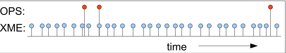
As mentioned before, the camera pose estimations are only available when the marker is detected by the camera, which result in very inconsistent measurements, see Figure 12 for a illustrative visualisation. This means that the filter has to deal with non-uniform multi-rate observations.

In [GSDR11] two solutions are very briefly mentioned. The first one is to synchronize to a higher order. The second is to weigh the uncertainty of each measurement with how often they occur. Nutzi et al [GSDR11] further developed the second solution, but simplified the weighing. They put the noise value of the measurements towards infinite if there were no recent measurements available. This results into almost completely ignoring those measurements. In [AM07] this goes one step further by only performing the prediction step of the filter. Thus completely ignoring the available measurements because others are missing.

In [SFD14] they mention synchronizing to the system update cycle. This is a popular choice in many systems, including navigation systems, industrial systems, and transportation systems, and others. The reason for it being that the fusion is often done on a central processing location.

[image:19.595.58.545.460.551.2]

For our model we use neither of those solutions. Instead we use a different update step for the XME and OPS observations. Then we apply the appropriate update as soon as we receive a measurement Figure 12: Illustrative visualisation of observations available over time. It is possible that that an OPS observation includes multiple observations.

time

XME:

(20)

from one of the systems. And because of the difference in frequency this means that it continuously gets updated using the XME measurements but infrequent and irregularly by the OPS. This is possible for our model as we don't need both observations to make an estimation.

XME only

If only a XME observation is present, the X, Z and yaw values are only predicted and left untouched in the traditional update step as we don't have any observation of these values. The prediction is done by using the value of the previous state and adding the predicted delta values. But after the update step updated delta values are available. This means that we can make a better estimation of the position values using: (22).

xposk = xposk−1+Δxposk

zposk = zposk−1+Δzposk

yawk = yawk−1+Δ yawk

(22)

For the covariance we use the same idea. The noise values of the estimated deltas is added to the noise values of the previous estimated positions.

OPS only

If only an OPS observation is present, the best estimate is the updated estimate of the update step.

OPS and XME

If observations of both systems are available at the same time, they are processed after each other. With the OPS observations(s) going first.

Multiple OPS observations

Next to different timings, the OPS can also deliver multiple poses at the same time. This can occur when multiple markers are identified in a single image. The maximum number of poses is

undefined. It can be defined how many are allowed in the filter, as it can be questioned how much (for example) a sixth pose has to offer for additional information. But Instead an approach is used that allows a variable number of observations. When multiple OPS observations are available at the same time they are concatenated together in the measurement matrix.

For example, if three OPS observations are available, we have 9 measurements in total. All three of the OPS observations are identical to (11). Each also have their own measurement error. (23), (24) and (25) show how the values are concatenated. The measurement matrix then looks as follows: Figure 13: Steps taken when only an XME observation is available. This corresponds with formulas: (13)(14) -> (15)(16)(17) -> (22) -> (21).

Predict

Update

XME only Correct position _{with deltas} Set speed, _Direction

Figure 14: Steps taken when only OPS observations are available. This corresponds with formulas: (13)(14) -> (15)(16)(17) -> (21)

(21)

M=

• See how the OPS error model performs compared to a simple static average.

A third pose estimator is used as a ground truth in order to compare the results. All three of the pose estimators record their measurements over a certain amount of time independent of each other (however the XME and OPS are recorded simultaneously in the same application). The same data is then reused in multiple experiments to keep the results comparable. An Optitrack system was used for this (http://optitrack.com/). The Optitrack system uses a set of infrared cameras combined with retro-reflective markers for its pose estimation. The Optitrack works independently on another system concurrent with the other pose estimators. The results of the Optitrack are compared with the results of the XME and the proposed model to draw conclusions. As the Optitrack measures at an independent rate, only the measurements that are closest within a maximum time frame of 100 milliseconds are used for comparison. There also exist a few gaps in the OptiTrack data where it was unable to track the user, for example if the user was walking outside of the tracking area.

4.1 Setup

For the experiment, four markers are placed on the ground in between the Optitrack cameras so both systems share the same tracking space. In this area data was captured for all three pose

estimators at the same time. A retro-reflective marker used by the Optitrack was mounted on top of the user close to the camera. After completing the data collection of the test run, the data of the XME and OPS is fed to the algorithm. The results of the fusion are then compared to the results of the Optitrack. There were no predefined patterns or movements. Although a few unusual

(23)

The duration of the test was 13 minutes and 35 seconds. The number of observations within a 100 time frame to a Optitrack observation are 85310 for XME and 2261 for OPS. In Table 1 the number of observations for each minute are displayed. On average the XME produces 104.8 observations per second and OPS produces 2.8 observations per second. The KF produces fewer than the XME because some of the XME observations are filtered out based on the time between the

measurements was sometimes lower than a single millisecond (or exactly the same).

1 2 3 4 5 6 7 8 9 10 11 12 13 14

XME 5251 5934 7200 7198 5293 5411 6895 5059 7199 7199 6919 7021 6951 1780

OPS 61 21 18 258 160 126 165 316 132 198 309 300 182 15

[image:23.595.86.344.53.356.2]

KF 4477 5278 6557 6711 4907 4724 5801 4336 6569 6720 6381 6493 6321 1559

Table 1: Number of observations that are within 100 milliseconds of a OptiTrack observation (each minute). There are less KF observations than XME observations because some of the XME

measurements have been filtered out because the time between the current and the previous measurement was too low. The 14th_{minute is not a whole minute, the recording was cut off}

[image:23.595.57.542.594.700.2]

somewhere in that minute.

(24)

4.2 Results

In general the results of the OPS weren't optimal in this test. There were easily noticeable bad pose estimations at certain points in the test. It was easily noticeable as the pose estimated by the OPS was jumping around while the other pose estimators displayed the user standing still. These jumps were caused by the OPS not correctly detecting the corners of the markers sometimes. After some investigation it can be explained by an error in the rectangle detection in in the pose estimation. It seemed that in some cases the detected corners were not of the marker itself but rather of the border of the sheet the marker is printed on. In Figure 16 an example of this behaviour is shown. It is unclear what causes this exactly as the marker is clearly visible in the binary image. A simple future solution for this is to increase the white space between the marker and the border of the sheet that the marker is printed on.

Besides those errors the results of the pose estimators still isn't impressive. In Table 2 the results are shown of the XME, OPS and also the KF (using the proposed method) compared to the OptiTrack results. Even though the overall numbers are high it still shows that the fusion does improve the results as the results for the KF are lower than those of the XME.

MEAN STD

XME 0.64 0.49

OPS 0.21 0.25

[image:24.595.130.334.223.332.2]

KF 0.22 0.35

Table 2: The mean and standard deviation in meters. (compared to the OptiTrack results).

XME delta model VS XME position model

[image:24.595.54.542.416.520.2]

We used an altered version of our proposed model so it could use the pose measurements directly instead of using the delta values. The changes entail: the observation matrix, which is now similar to that of the OPS. The second change is how the speed and direction after the update step is set is calculated, because the model doesn't receive updates for the delta values any more. Instead it now calculates the speed and direction based on the difference between the current and previous filtered results. We did two tests with this altered model. One with the XME keeping the same noise model as the XME noise model used in the proposed model. With the other we use an accumulative noise model for the XME that better displays the expected noise for the XME pose measurements. In this test we accumulate the noise vales of the XME measurements per observation. Because the XME position value is expected to contain more noise over time, this noise model will reflect that to the filter. This test is done to confirm the challenges mentioned and see if the proposed method works better.

(25)

In Figure 17 the results of test with the low XME noise values are compared to the XME

measurements to show that the results are very similar. This approach has little to no improvement over the raw XME measurements.

[image:25.595.72.526.122.379.2]

The data in Figure 18 is an comparison of the same test but now with the accumulated XME noise model. We again made the comparison with the XME measurements to look for improvements. Here it looks like like there is some improvement in the averages when looking at minutes 8 to 12. But the increasing standard deviation over time shows that the results become more unstable the more time passes. There is also the abnormality in 13th_{minute where the error on the filter results} became very high. This seemed to be because the speed and direction update was large in one case, which caused the predictions to be large as well. Normally if this would happen the filter would correct itself with the following measurements, but because the expected noise on the XME measurements had became higher than the prediction noise, the filter had trouble correcting itself.

Figure 17: The kalman filter results when using the XME pose data directly with a low noise model compared to the raw XME output.

1 2 3 4 5 6 7 8 9 10 11 12 13 14

0 0.2 0.4 0.6 0.8 1 1.2 1.4

Kalman filter results using XME position data with a low noise model

XME KF

Individual minutes

E

rr

o

r

in

m

e

te

(26)

In Figure 19 a part of the result of the two tests are shown in comparison with the Optitrack and raw XME data. It shows how the results don't seem to improve over the raw XME data.

OPS noise model

[image:26.595.71.529.70.325.2]

We compared the results using the proposed Delta model with two different noise models for the OPS measurements. We compare a standard deviation and the proposed OPS noise model. We claim that the proposed model would better represent the noise on the measurements and thus lead to more accurate results. In Figure 20 it is visible that using the proposed noise model on average leads to slightly better results. The overall average for the standard deviation method is 0.237 ± 0.093 and the for the proposed (pixel) method 0.206 ± 0.087.

Figure 18: The Kalman filter results when using the XME pose data directly with an accumulating noise model compared to the raw XME output. The error measured of the Kalman filter in the 13th_{minute is higher than depicted here, but the chart is cut off at 2}

meters.

1 2 3 4 5 6 7 8 9 10 11 12 13 14

0 0.2 0.4 0.6 0.8 1 1.2 1.4 1.6 1.8 2

Kalman filter results using XME position data with an accumulating noise model

XME KF

Individual minutes

E

rr

o

r

in

m

e

te

rs

Figure 19: The four images are of lines drawn through all the postiion data in the 10th_{minute. The}

[image:26.595.60.539.424.581.2]

(27)

Drift correction

We compare the results of the proposed delta model with the proposed OPS noise model with the XME measurements to see if the results of the extended Kalman filter don't suffer from the same drift that is present in the XME measurements.

In Figure 21 it is visible that the mean error of the XME measurements rises over the duration of the experiment. For the Kalman filter results the mean error doesn't seem to rise. The mean error at the first and last minute are very close. This suggests that the Kalman filter results do not experience the same drift as the XME does.

[image:27.595.69.525.60.311.2]

What also seems interesting are the values at minutes 6 and 7. The means are much higher for the XME results there. This can be explained by the movements of the user at that time. At that time the user sat down on an office chair and rolled across the room and back. The fact that we returned back at the same point where we started explains why the high increase in error subsides again.

Figure 20: Mean error for the Kalman filter results. One using the error model based on the number of pixels the marker is represented by and the other with a static number (the standard deviation).

1 2 3 4 5 6 7 8 9 10 11 12 13 14

0.00 0.10 0.20 0.30 0.40 0.50 0.60 0.70

The kalman filter results when using the standard deviation and the proposed error model based on the number of pixels

STD Pixel

Individual minutes

E

rr

o

r

in

m

e

te

(28)

After comparing the mean XME error at the start with the mean error at the end of the test there seems to be a drift of 4-5 centimetre per minute. This approximation should not be taken as a standard drift for the XME, it is highly likely the drift was artificially introduced. Although it can happen and our purpose was to illustrate how the XME alone cannot recover from it.

[image:28.595.68.529.53.319.2]

In Figure 22 our different results are summarized of the experiments with the standard pose XME measurements (the blue and the red) and our proposed method (yellow). In this comparison one can clearly see that the proposed method performs better.

Figure 21: Mean errors for the XME, OPS and KF positions compared to the OptiTrack measurements. The results are calculated separately for each minute.

1 2 3 4 5 6 7 8 9 10 11 12 13 14

0 0.2 0.4 0.6 0.8 1 1.2 1.4

Mean error compared to the Optitrack seperate for each minute

XME OPS KF Individual minutes M e a n e rr o r in m e te rs

Figure 22: Kalman fitler results using XME position data instead of the proposed delta XME data. 2 different noise models are explored. The results of the proposed method are also included for comparison.

1 2 3 4 5 6 7 8 9 10 11 12 13 14

0 0.2 0.4 0.6 0.8 1 1.2 1.4 1.6 1.8 2

Kalman Filter results when using the XME position with different noise models

[image:28.595.73.524.469.741.2]

(29)

5 Discussion

Several tests have been done to get an idea on how the proposed method performs. In this chapter we are going to discus these results.

Delta approach vs position approach

The Kalman filter results when using poses for XME observations with a low noise model are basically the same as the XME results. This is as expected because we are basically telling the filter that the XME is very accurate. The OPS measurements have a very small influence because the next XME measurements will undo any changes made.

The second test used the error model that increases in the expected noise by accumulation the observation noise over time. The results seemed to be more accurate than the XME measurements by themselves. Although in the thirteenth minute the error skyrocketed. It is also expected that the accuracy will get worse over time. The standard deviation on the errors seems to grow over time, which means the results become less stable as can be seen in Figure 19. Besides these drawbacks the results are also worse than the proposed method (Figure 22) in general.

Multi-rate

The corrections are only done when OPS observations are available. So it is not continuously corrected. And the corrections are also dependant on the quality of the observation. Inaccurate OPS observations can hurt the results more than correct. In Figure 21 it is visible that the Kalman filter results are still very much dependant to the XME results. This is visible by looking at the 6st and 7th minute, where the filter's error is much higher than the OPS measurements error. So if the XME measurements are faulty, the Kalman filter will give inaccurate results. However, the algorithm is able to recover if the XME measurements become accurate again and OPS measurements are available.

Noise model OPS

Comparing our approach for the error model of the OPS with the standard deviation (Figure 20) reveals that our model doesn't give a big improvement. This isn't a very surprising result

considering the data set used. Because the pose estimation algorithm itself already has an upper limit where it will detect markers so does the error associated to it. This means that the error of our approach will never deviate far from the standard deviation. If the maximum marker detection range would be increased, a higher improvement would be expected from the proposed noise model compared to the static noise model.

Drift

The average results per minute (in Figure 21) show that while the XME error keeps getting larger over time, the error for the Kalman filter results stays more or less the same. This suggests that the fusion corrects the drift. What is interesting is that in the fourth and fifth minute the OPS

measurements are worse than both the XME and the Kalman filter results. It is expected that the Kalman filter results can only reach the accuracy of the OPS measurements. So if if the OPS measurements are less accurate than the XME measurements, the Kalman filter is expected to produce worse results than the XME measurements. This is expected because the OPS

measurements would 'derail' the results by trying to correct the XME with less accurate

(30)

6 Conclusion

In this work a sensor fusion algorithm based on the extended Kalman filter is used to correct the drift for pose estimation. The algorithm fuses together two independent measurements from two different pose estimation systems, the XME and the OPS. The delta model used to align the coordinate systems allows these systems to fuse together rather than to compete with each other. The use of two different update steps that can be used individually circumvents the need to synchronize the measurements for the filter. An implemented restriction in the marker detection limits the usefulness of the measurement-based noise model for the OPS, resulting in only slight differences compared to the static noise model. Overall it is shown that the algorithm corrects the measurements of drift when comparing the results of the fusion algorithm with the results of a third party pose estimator.

7 Future work

As the overall goal was to improve the existing system by eliminating the drift, much effort went into the fusion of the measurements instead of the accuracy of the measurements themselves. So there are lots of improvements available that weren't implemented in this work. For example: the offset between the camera and XME head poses are

roughly estimated in this research. Just as the several noise values in the Kalman filter. But there exist algorithms to calculate these values.

Furthermore the accuracy of the OPS can improve as well, in the recorded data we encountered cases where the marker detection incorrectly found the

dimensions of the marker. These incorrect dimensions resulted in an inaccurate pose. So further marker detection improvements are recommended.

The applicability of the system in the application setting isn't tested. So it is unknown how well it performs in a real case. Will the algorithm correct often, fast and accurate enough to be dependable? The next step should be to test how well the the current system performs in the application setting. The focus of the test should be to find out if the system is reliable enough for users to prevent accidents caused by the misalignment of coordinate systems.

[image:30.595.326.533.251.408.2]

There also remains the subject of how the correction is performed. Should the users be immediately corrected to the best estimated position or should there be a transition period towards that (which will slow down the correction rate). Or should the correction only take place when a user is moving to make the changes feel less sudden? Several methods could be tested on users to see what they experience the most comfortable. And possibly there could be looked at a trade-off between the accuracy and comfort.

(31)

References

KMYWJ05: K. Kim, M. Lee, Y. Park, W. Woo, J. Lee, ARPushPush: Augmented Reality Game in Indoor Environment, 2005

CMD14: C. Forster, M. Pizzoli and D. Scaramuzza, SVO: Fast semi-direct monocular visual odometry, 2014

JTD14: J. Engel, T. Schöps, D. Cremers, LSD-SLAM: Large-Scale Direct Monocular SLAM, 2014 SN06: S. Hesameddin, N. Shoushtari, Fast 3D Object Detection and Pose Estimation for

Augmented Reality Systems, 2006

SILT12: S. Siltanen, Theory and applications of marker-based augmented reality, 2012 STOR12: J. Stork, Camera pose estimation with circular markers, 2012

AJD11a: A. Pagani, J. Koehler, D. Stricker, Circular markers for camera pose estimation, 2011 ACJ05: A. Rice, C. Cain, J. Fawcett, Dependable Coding of Fiducial Tags, 2005

SRFM14: S. Garrido-Jurado, R. Muñoz-Salinas, F.J. Madrid-Cuevas, M.J. Marín-Jiménez, Automatic generation and detection of highly reliable fiducial markers under occlusion, 2014 FIAL05: M. Fiala, ARTag, a fiducial marker system using digital techniques, 2005

DD07: D. Wagner, D. Schmalstieg, ARToolKitPlus for Pose Tracking on Mobile Devices, 2007 AJD11b: A. Pagani, J. Koehler, D. Stricker, Detection and Identification Techniques for Markers Used in Computer Vision,

KALM: R. E. Kalman, A New Approach to Linear Filtering and Prediction Problems,

GSDR11: G. Nützi, S. Weiss, D. Scaramuzza, R. Siegwart, Fusion of IMU and Vision for Absolute Scale Estimation in Monocular SLAM,

AM07: A. Smyth, M, Wu, Multi-rate Kalman filtering for the data fusion of displacement and acceleration response measurements in dynamic system monitoring, 2007

Drift correction using a multi rate extended Kalman filter