The impact of predictive inaccuracies on execution scheduling

http://wrap.warwick.ac.uk/

Original citation:

Jarvis, Stephen A., 1970-, He, Ligang, Spooner, Daniel P. and Nudd, G. R. (2004) The impact of predictive inaccuracies on execution scheduling. University of Warwick. Department of Computer Science. (Department of Computer Science Research report).

Permanent WRAP url:

http://wrap.warwick.ac.uk/61313

Copyright and reuse:

The Warwick Research Archive Portal (WRAP) makes this work by researchers of the University of Warwick available open access under the following conditions. Copyright © and all moral rights to the version of the paper presented here belong to the individual author(s) and/or other copyright owners. To the extent reasonable and practicable the material made available in WRAP has been checked for eligibility before being made available.

Copies of full items can be used for personal research or study, educational, or not-for-profit purposes without prior permission or charge. Provided that the authors, title and full bibliographic details are credited, a hyperlink and/or URL is given for the original metadata page and the content is not changed in any way.

A note on versions:

..$$rH."ro,

effi

r&?

wAryrct<

Research

Report

3go

THr

In,tpncr

or

pneDrcrvE

_lrunccuMcrEs

_oN

Execuloru

ScnEDULtNG

Stephen

A Jarvis,

Ligang

He,

Daniet

p

Spooner

and

Graham R Nudd

The

Impact

of

Predictive

Inaccuracies

on

Execution Scheduling.

Stephen

A.

Jarvis, Ligang He, Daniel P. Spooner and Graham R. Nudd

High Performance Systems Group, Department of Computer Science,

University of l|/arwick, Coventry CV4 7AL, UK

Email : [email protected]

Tel: +41 (0)2476 _{524258 Fax: +41} (0)2476 573024

Abstract:

This paper investigates the underlying impact of predictive inaccuracies on

execution scheduling,

with

particular

reference

to

execution

time

predictions. This

study is conducted

from two

perspectives: from that of

job

selection and from that

of

resource allocation,

both

of

which

are fundamental components

in

execution

sched-uling.

A

new performance metric, termed the degree of misperception, is introduced

to

express the

probability

that the predicted execution times of

jobs

display different

ordering characteristics

from their

real execution times due

to

inaccurate prediction.

Specific formulae are developed

to

calculate the degree

of misperception in

both

job

selection and resource

allocation

scenarios. The oarameters

which

influence the

de-gree

of misperception

are also extensively investigated. The results presented

in

this

paper are

of

significant

beneflt

to

scheduling approaches that take into account

pre-dictive

data; the results are also

of

importance to the application

of

these scheduling

techniques to real-world high-performance systems.

Index terms:

performance prediction, execution

time,

scheduling,

job

selection,

re-source allocation, and performance evaluation

-

This work is sponsored USARDSG, contract no.

in part by grants fiom

N6817r-01-C-90l2),

the NASA AMES Research Center (administrated by

1.

Introduction

Scheduling

in

a single processor environment is, at its most basic level, the task

of

determining

the

sequence

in

which

jobs

should be executed.

In

a multi-processor or

multi-computer environment on the other hand,

job

scheduling also involves the

proc-ess

of

resource allocation, that is, determining the resource

to which

a

job

should be

sent

for

execution. The design

of

scheduling policies

for

parallel and distributed

sys-tems has received a good deal

of

attention

_12,4,5,14,

15]. These schemes are often

based

on the assumption

that

the

job

execution times are

known

somehow

_[5,

9].

While

this

is

a useful assumption

to

make, information

of this type is often unknown

and must therefore be

obtained

through

some

predictive mechanism.

A

naive

ap-proach to this problem

might

be to require the owner of the

job

to estimate the

execu-tion time

based on their past experience.

A

more sophisticated approach

might

be to

utilize

performance

prediction tools

to

perform this function.

A

number

of

increas-ingly

accwate prediction tools have been developed that are able to predict the

execu-tion

times

ofjobs

based _{on performance models [3, 6, 7,} 8] or historical data _[1, 13].

In

spite

of

this,

an inevitable fact is that the prediction results are

unlikely to

be

entirely

accurate and as a result, this may have a fundamental impact on

job

selection

and resource allocation.

In

the case

ofjob

selection, the inaccurate prediction may mean that the scheduler

has an incorrect

view

of the order in which

the

different iobs should

execute. For

ex-ample,

it

may be the case that the real execution time of

job

_-[

is greater than that

of

job J2; because of the inaccurate prediction however, the scheduler may view

job

-L as

having a shorter execution time than that of

job

-/2. Therefore,

if

the scheduling

policy

is based on

job

execution times (the shortest

job

serviced

first, for

example), then this

misperception

will

impact on the order

in which jobs

are selected

for

execution. This

will

ultimately influence

the scheduler and system performance.

When a scheduler receives a

job

in a parallel or distributed system, there may be a

number

of

resources (processors

or

computers) available

on which

the

job

may

be

executed.

If

the resource

allocation

policy

is also

based

on the

expected execution

time of

the

job

on the

different

resources (select the computer that offers the shortest

execution time, for example) then these inaccuracies might also cause the scheduler to

wrongiy

select between them. Again, this misperception

will

impact on the scheduling

and overall system performance.

The existence

of

misperception originates

from

the

inaccurate

prediction

(of

in

this

case execution

time), and should

be viewed as an inherent characteristic

of

any

prediction-based scheduling scheme that operates

in

a highly-variable real-world

sys-tem. This said, different scheduling policies

will

have different levels

of sensitivity

to

the degree

of misperception.

Thus, the study of the impact of inaccurate prediction on

scheduling performance can be decomposed into two levels

_-

at the underlying level,

as a study into the degree of misperception originating from inaccurate prediction; and

at the higher level, as a study into the sensitivity

of

individual

scheduling policies to

this

degree

of misperception. This

paper addresses the former, where the latter is the

subject

of future work.

Different

predicted errors can lead

to different

degrees

of

misperception. The

ob-jective

of this paper is to establish the relationship between the predicted error and the

degree of misperception, for both

job

selection and resource allocation scenarios. This

study provides an

insight into

the underlying impact

of

inaccurate prediction on

job

selection and resource allocation and

significantly benefits

the design and evaluation

The rest

of

this paper

is

organized as

follows.

Formula

for

the degree

of

misper-ception, and

forjob

selection and resource allocation are developed

in

Section 2. The

parameters that influence the degree

of

misperception are then extensively evaluated

in

Section 3. The paper concludes

in

Section 4.

2.

An

Analysis

of

the Degree of

Misperception

2.1

Job Selection

When performance

prediction tools

are used

to

estimate the execution times

of

jobs,

the predicted execution time usually lies in an interval around the actual

execu-tion time (of

the

job)

according to some _{probability distribution [7,} 8].

Suppose that the actual execution

time

of

job

Ji

is

xi

and that the predictive error,

denoted by y;, is a random variable in the range

I

o*,,bx,]

following

some probability

density function,

gi\);

where the possible value fields of a and

b are

_[0,

100%] and

[0,

-),

respectively.

It

is assumed that the predictive errors

of different jobs

are

inde-pendent random variables. The predicted execution

time

of

job

-/,, denoted

by zi,

is

computed using Eq.1.

Zi=Xi+yi

(1)

Suppose two jobs

Jt

and Jzhave the actual execution times

xt

ard x2, where

xtlxz.

Then the predicted execution times of -rl and Jz, that is zr and 22, a;te

xfyl

and

xzflz,

respectively.

Given

that x

_t*1

a misperception happens

if

z

r):2.

The degree

of

mis-perceptionfor

these two

jobs,

denoted by MD(x1,x2), is defined by the probability that

zP-:zzwhlle xt-. ..xz. This probability is denoted by P,(zps2lx,<xz).

With

Eq.1. this

prob-ability

can be further transfbrmed using Eq.2.

P,(z pz2lx

_fxz):P,(x

;y

12 x2*y2lx

_fxz):P,(y

P- y2+x 2-x

I

xz-

x

P0)

(2)

MD(x 1, x

z):

P,(y t> y 2+x 2-x tl x _2- x

P0)

(3)

From Eq.3,

it

can be seen that the probability that the misperception happens is the

probability

that given x2-xpQ, the predictive error

of

I

(i.e.,

yr)

is

greater than the

predictive error of

4

(i.e.,

yz) plus the difference between x2 and

xt.By

constructing

the coordinates of the

predictive

error

yr

andyz, the inequality ypy2+x2-x7 means that

y1 and _)t2 are given values from the area above the line

_!

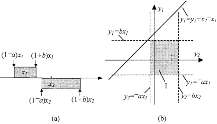
F!z-rxz-x1.

Fig.

i.a, 2.a

and 3.a illustrate the relation of predicted execution times of

Jt

and Jz,

while Fig.1.b,2.b

and 3.b show the corresponding value fields of the predictive error

of .rr and Jz

(yt

andy2) as

well

as the corresponding area in whichy7)42*xz-xt.

t\

rVt:VtrX>

Xt

I I

\*

I

!i:r:iil :::i:l:l

:l,:ill lri:t;l

--i\--

_{_}

t, \t:

axl

t\

i Vt:DX>

(I-a)x2

Q+b)x2

[image:7.595.111.468.349.553.2]

(a) (b)

Figure.l.

Case

study

1

(a) the predicted

execution

times of jobs

Jt

and,I:

do not

overlap; (b) the corresponding coordinate

area

which the predictive

errors

yl

andy2 can

be assigned values

from.

Fig.1.a illustrates the case when the ranges

of predicted

execution times of -L and

-/z do not overlap.

In

this

case a misperception

will

not occur

even

if

the predictions

are

not

accurate. Correspondingly,

Figl.b

shows the coordinate area

of

the predicted

errors of -L and J2 (arca

I), which

is the area surrounded by the

lines:yr:-ax1,))fbxr,

!z:-ox2

and

y2:bxz.

As

can be seen

from

the figure,

all of

area

I

is below the line

/F/z*xz-xl.

Hence,

P,(yP

y2+x2-xtl

x2-

xp})

inEq2

is

equal

to

zero.

This

case is

expressed more

formally

below.

P,(yp

y2+xz-xl xz-

x7>0):0

_{-ax2>-bx1*x2-x1,}

x2-xp0

(4)

(l-a)x

1

(l+b)xl

(I-a)x2

(l+b)x2

(a) (b)

Figure.2.

Case

study

2 (a)

the predicted

execution times of

jobs

Jt

^nd.:I2 overlap,

however the lower

limit

of the predicted

execution

time for

Jz does

not

cover x7i

(b)

the corresponding coordinate area of predicted

errors

of

.Il

and Jz

_Ot

and yz)

in

which

the misperception occurs (the area is a

triangle).

Fig.2.a illustrates the case when the predicted execution times of _{-rr and} J2 overlap

and the lower

limit

of

the predicted execution time of Ju is greater than

xr.

The

cone-sponding coordinate atea of y 1

^d

yt

is shown

in Fig.2.b

(area

I). In

area

I,

part of the

area

is

above the line

_lFlztxz-xr

(area

II),

which is itself

surrounded

by

the three

lines: y7:bx i,

_!2:-ffi2

and y

py2*xz-xl.

When

_!1

and

lz

are assigned values

from

area

lI,

y1 andy2 satisfu y12y2-rx2-x7, that

is,

a misperception

will

occur; a misperception

will

not occur

if

y7 and

lz

are assigned values

from any

other area

in

I,

although

pre-diction

errors

will

still

exist. The

probability in

Eq.2 equals the double integral of the

probability

density

functions

of

predicted errors (i.e.,

gtOt)

and g2Q2))

on

area

II,

which

is calculated

in 8q.5.

v

r:bx

t

P,0

_P

y 2+x 2-x tl x 2- x p0

_):

l::,,_,. _

r,l^

j

"-'"

g' ( y ₎ g z(y z) dy zdy t

- ax

r(x

_z-x 1)<- ax 2<b x

r(x

z-x r), x-.-x 7>0 r5)

(l-a)x

1 (1+b)xt

(l-a)x2

(l+DJX_r

_!Z:

ax:

II

Figure.3.

Case

study 3 (a) the predicted

execution times of jobs

Jr

and _"/2 overlap

and the lower

limit

of predicted

execution

time of

aI2 covers

xu; (b) the

corre-sponding coordinate area of predicted errors

of

_-/i

and Jz

_Ot

and

_/z)

in which

the

misperception

occurs (the area is a

trapezoid).

Fig.3.a illustrates

a

third

case when the predicted execution

times of

Jt

and Jz

overlap. The dilference

from

Fig.2.a is that the value

field

of

J:'s

predicted execution

time

covers

x7. The

corresponding coordinate area

in

which

_!1

and

y2

satisfy

yp42*xz-x7 is highlighted

as area

II

in

Fig.3.b. The area

is

a trapezoid rather than a

triangle

as

in

Fig.2.b. The formula

for

calculating the

probability in Eq.2 is

also

dif-ferent from Eq.5; this is shown in Eq.6.

P,$,, 12 y 2+x z-x tl x

z-rr

t0):

l*,

y

r-(x z- x r)

g

_{y)

g z(y z) dy z dy t

-ax z3-ax

r(x

z-x t),' xz-x

P0

(6)

Eq.4-6 account

for all

possible relations between the predicted execution times

of

Suppose that the

probability

density function

of

a

jobs'

actual execution

time m

a

job

_stream

_isfix)

_and

_thatthe

value

field

of the real

executiontimex

is

_[x/,

xu].The

degree of misperception of this

job

stream, denoted bV

MD,

is defined by the average

of

the degree

of

misperception

for

any two

jobs in

the

job

stream

.

MD

is computed

using Eq.7, where MD(x1,x2) is computed using Eq.4-6.

MD

= _f:,'

_f:

f

Qr)f

(xz)MD(xr,xz)dx:dxr

There are several independent parameters in Eq.7, as

well

as in Eq.4-6: a, b, xu,

xl,

f.r),

and

gi(xi).It

is

highly

beneficial

to

study

how

these parameters influence the

value

of

_Un;

this is the subject of the investigation in Section 3.

2.2 Resource allocation

In

dedicated environments, the execution time

of

one

unit

of

work

can be

repre-sented as a predicted

point

value

_[0,

11,I2].

However,

in

non-dedicated

environ-ments. the existence

of

background workloads on the resources causes a variation in

unit

execution times

_[3,

10, 11,12]. Hence

it

can be assumed that the actual execution

time

of

one

unit

of work

locates across a range around the predicted point value

fol-lowing

a

certainprobability

_[10, 12, 16].

Suppose there is a distributed system consisting

of

n heterogeneous computers c7,

c2,

..., c,.

Computer c;

is weighted

wi(l<i3n),

which

represents the time

it

takes to

perform

one

unit

of

computation.

Now

suppose

fbr

any i,

i

(l<i,i<n),

wi<wi

if i<i. A

job with

size s is therefore predicted to have the execution

time swi on

computer c;.

The predicted execution time of a

job

is denoted by

,,,,that

is,

(7)

However,

in

shared environments the actual execution

time

for

a

job with

size s

on computer c;

ma/

not be,sl.r/i, because of the existence of background workload. The

actual execution time of a

job

on c; is therefore denoted by *",.

For

a

job with

size s,

its predicted error on computer

c;, denoted by _"vci, iS

com-puted using Eq.9:

(e)

Suppose

y,; falls in

the range

_{l-sw1xa,.vlr,xb]}

following

the probability density

function

gri(!"i).

Hence, x"; locates in the range

_[sw;x(l-a),

s]r,x(1+b)].

For

two

computers

ci

and cy, suppose

thatwfw.,.

Then, the predicted execution

time

of

a

job with

size s on c; and c; satisfu sw1<s1v . However, the range

of

the

job's

actual execution time on computer c;

is

_[sw;x(l-a),

swix(1+b)] and may overlap with

that on computer cr,

which is [sw;x(1-a),

sw.,x(l+b)]. Consequently, the actual

execu-tion

time on computer

c;

ma)

be greater than that on

ci.In

this

case, the inaccurate

predictions cause a misperception in the order of the actual execution times on these

two

computers. Depending on the

individual

scheduling algorithm, this misperception

may lead to the wrong selection

of

a computer to which the

job

is sent.

Similarly,

the

degree of misperceptionfor a

job

with

size s on two computers ci and c7, denoted by

MDr(ci,

c;), is defined

by the probability

thatx,/s".1while

zcilZcr.

This probability

is

denoted

by P,(x,/s"ilz"i<z), which

can be further transformed

by Eq.t0 with

Eq.8

and 9.

P,(x"/s"ilz";<z"i):P,(zrr!ri)- zrr-yrilzrfzr):P,(Jrt2

yci+swt-sw1l

wt-

w/0)

(10)

That is,

MD,(ci,

cy) is computed using the

following

equation:

Applying

a

similar method to that

used

to

compute MD(x1, x2), the equation for

computing MD"(ci, c;) is expressed

formally

as foliows.

MD"(c,"r=

{

bswt 1 _-aswi

*

s(w1

_-wi)

pbvt-s(wi-wt) pbyt

|

|

B"(y",)gq(y4)dydy,,

J-aw' J ya+s\uJ-w ₎

-

asrri+ s(w7

-

wi) < bswt < bsw, + s(w1

_-

w,)

?DSWi tD9i

| |

g,,ly,,)g,1(y"1)dy,1dy", bswl 2 bswi +

s(wi-

w,) J-aswt Jyct+slwJ-wt)

1n-ln

MD.=

+t

_\,MD,7c,.c,1

f- z .? t_t v 2 t=l 1=11'1

(r2)

The degree of misperception

_for

a

job

with size s

for

n heterogeneous computers

ct,

c2,

...,

cn,denoted

by MD,,

is defined using the average of the degree of

misper-ception for the

job

on any two computers, which can be computed using Eq.13.

(13)

3.

An

Evaluation

of

the Degree

of

Misperception

In

the previous section the general formula

for

the degree

of

misperception

for

both

job

selection and resource allocation were presented.

In

this

section an

investi-gation is

conducted as

to how

the parameters

in

these formulae impact on the value

assigned to the degree of misperception.

3.1

Job Selection

The parameters

a

and b represent the range

of predicted

errors

in Eq.4-6.

Fig.4.a

and Fig.4.b show the impact of the parameters

a

andb on the value

_Un

.

tt

is difflrcult

to

evaluate the impact

of

these parameters

if

the probability density

function of

pre-dicted enors

takes a general

form.

Therefore in the

following

parameter evaluation,

the predicted error

for

the execution time of

x

is

assumed

to

follow

a

uniform

8,\!')

=

(b +

a)x

Three types of

job

stream are investigated. The actual execution times

in

these

job

streams

follow

a

uniform,

Bounded Pareto and Exponential distribution, respectively.

Theirprobability

density

functionsfx)

are shown

in

Table

1.In

the

job

stream

fol-lowing

the exponential

distribution,

the

job

execution time has no upper

limit.

Only

execution time values

in

_[10,

14.6] are considered, as 99o/o

of

the execution times

lo-cate

in this

range according

to its probability

density

function. This simplification

does not impact on the accuracy of the results.

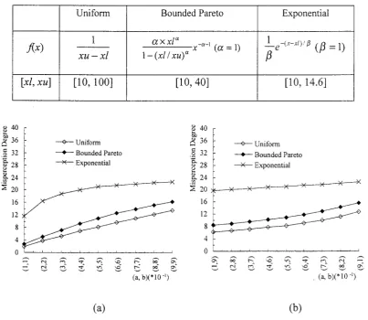
Table

1.

The range

of

job

execution times

in

the three

job

streams

40 36 28 1A 20 l6 t2 8 A 0

(a)

(b)

Figure.4.

Impact of

the parameters

s

and

b on

_l,tO

(a) the

impact of

the range

size of predicted

errors

(b) the impact

of the range location of predicted errors

u40 436 H o)z '5 Srn 9. rn

5zo

16 12 8 .l 0 o O o N6Sh€rqo N-Vn€r€o

/a h\/*lA'l\

Uniform Bounded Pareto Exponential

JU)

1

xu-

xl

e,x

xl"

_-n-t .

-x'

\u=t)

l-(xl

I xu)"

lxl,

xu] [10, 100]

[10,40]

[10, 14.6]

---+- Uniform

---i-

Bounded Pareto

--x-

Exponential

---9- Uniform

--f-

Bounded Pareto

[image:13.595.97.501.358.708.2]

In

Fig.4.a,

a

and

b

increase

from t0%

to

90o/o

with

increments

of

10%. This

means that the range

of

predicted

error

for

the actual execution time of

x

increases

from

_[-0.lx,0.lx]

to

_{[-0.9x,0.9x],}

while

the

average predicted

error remain

un-changed (at 0).

As can be observed

in Fig.4.a,

under all three

probability

distributions, the degree

of misperception increases as a and b increase. This is because as a and b increase the

predicted execution times of

jobs

have a higher probability of overlapping

with

each

other, which leads

to the overall

increase

in

UD.

This result suggests that when the

average predicted error is the same, the range size of predicted errors is

critical for

the

value

of

tvfD.

It

can also be observed that under the same

a

and b, the degree of misperception is

highest under the exponential

distribution,

second highest under the Bound Pareto

distribution

and the lowest under the

uniform distribution. This is

because the size

of

the range

of

actual execution times is smallest when the execution times

follow

an

ex-ponential distribution and the largest when

following

a

uniform

distribution. This

re-sult

suggests that the actual execution times

will

also influence the degree of

misper-ception. This is demonstrated in Fig.5.

In

Fig.4.b, the range size

of

the predicted error

for the

actual execution

time of x

remains unchanged (at

x), while

the location

of

the range shifts towards the

left from

[-0.lx,

0.9x]

_{to [-0.9x, 0.lx].}

The result of this is that the degree of misperception

in-creases as the range

location shifts leftwards

(see Fig.4.b). The reason

for

this is

as

follows.

Consider Fig.2.aand Fig.3.a. When (a, b) rs (0.1, 0.9), the range of predicted

errors for xr and x2 ait? _{[-0.1x7, 0.9x7] and [-0.1x2 ,0.9x2],} respectively. The size of the

range where the predicted execution times for xr and rc2 overlap is

When

(a,b)

is (0.9,0.1) however, the range of predicted errors are _{[-0.9x7,0.1x7]} and

f-0.9x2,0.Lx2f, respectively, and the size of the overlapping ranges is

0.9x2+0.lxrkz-xt)

Since x2 is greater than x7, hence,

0. 9xr+0. I x _{2-(x 2-x 1)<0. 9x2+0.} lx

_7(x

_2-x 1)

this means that in general the size

of

the overlapping ranges

is

greater when (a, b) ts

(0.9, 0.1) than when (a, b) is (0.1, 0.9). This therefore leads to the increased degree

of

misperception.

This result

suggests that compared

with

an overestimation

of

execu-tion time, the

same level

of

underestimation may result

in

a higher degree

of

misper-ception. o40 i^ oJo aJ' .E g26

R rr

5ro

lo t2 8 4 o40 O

Fo

-.

AJO H AJL '5 Szs Ltd Ezo i6 t2 8 4 0 O\€r\On$Oal No.f,n€r€o, \or€o10NO$ i:-{: Nca$ocooo h€r€c\ (a)

Figure.S.

The impact of actual

execution times on the degree of misperception (a)

the

impact

of the range size

of actual execution times

(b) the impact

of the range

location of actual

execution times

(b)

---l- a h:O Q

---_6- _' . h:n qv v.J<

---<!- r h:O I

---l- a h=0 Q

----6- q h=n s

Fig.5.a and Fig.5.b show

the impact

of

actual execution

times on the

degree

of

misperception. The results show the data

for

the actual execution times

following

a

uniform

distribution; the results

for

the Bounded Pareto distribution display a similar

pattern. This study does

not

consider the execution times

with

an exponential

distri-bution,

since

their range

size

(xu-xl)

is fixed

when 99o/o

of

the execution times are

considered.

Fig.5.a shows

the impact

of

the size

of

the range

of

actual execution times (i.e.,

xu-xl).In

this same figure, the average of the actual execution times remains the same

(at

100)

while

the range size

of

execution times decreases

from

180 to 20

with

decre-ments

of

20. This experiment is conducted

with

different values

of a

and b.

It

can be

observed

in

Fig.5.a that

for

the

same values

of

a and

b,the

degree

of

misperception

increases as the range size decreases. The reason

for

this is

as

follows:

as the range

size

of

the actual execution times decrease, the value

of

x2-x1(in

Fig.2.a

or

Fig.3.a)

decreases on average under the same

a

and b. As a result of this, the overlapping area

of

the two predicted execution times increases,

which frnally

leads

to

an increase

in

tttn

.

tt it

result

suggests

that when the

average execution

times are

the

same, a

greater variance

in

execution time is of benefrt, as this

will

reduce the degree of

mis-perception.

Fig.5.b

demonstrates the impact

of

the location

of

the range

of

actual execution

times. In Fig.5.b, the range size

of

execution times remains constant (at 50) while the

range shifts

from

_[10,

60]

to

_[90,

140].

As

can be seen

in Fig.5.b,

the degree

of

mis-perception increases

in all

cases as the range location shifts

from

_[10,60]

to

_[90, 140].

The reason

for this

is that

as the range

location shifts, the

mean execution time

in-creases. Under the same

a

and b, the larger the actual execution

time,

the greater the

have

higher probability

of

overlapping

with

each other, which then incurs a higher

degree

of

misperception.

This result

shows that when other parameters remain

con-stant, the

job

stream

with

the greater average execution time tends to cause the highest

degree of misperception.

3.2 Resource allocation

In

Eq.12 and 13, the parameters that influence

MD,

include

the error

range

pa-rameters

a

and b, the computer weight w

_i

and the

probability

density function of

pre-dicted errors

g"i(!ri).

in

the

following

experiments, the values

of

these parameters are

given in Table 2 unless otherwise stated.

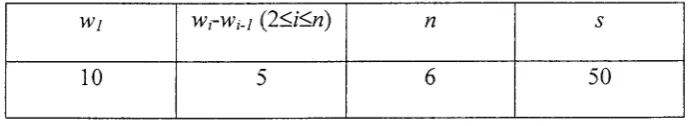
Table

2.

The default values of the parameters

for

the experimentation

W1 wi-wi-r

_Q<i<n)

n s

10 5 6 50

In

the

following

figures, the predicted error for the execution

time of

x

is also

as-sumed

to follow

a

uniform

distribution

in

_l-asw6

bsw;], whose

probability

density

function

g,i(!,i)

is expressed as follows:

g"i(y"i) =

_i"*,

The parameters

c

and b indicate the range of the predicted error. Fig.6.a shows the

impact

of

the range size

on WA

.

The result has a similar

pattern

to

that

seen in

Fig.4.a, which suggests that the range size

of predicted errors is also critical

for

the

value

of

MD.

Similarly

to

Fig.4.b, Fig.6.b demonstrates the impact

of

the range

lo-cation

on MD,. In

the study

of

resource

allocation,

_lsw{I-a),

sw;(l+b)]

represents

[image:17.595.125.470.374.437.2]

to (9,

1) means that the predicted execution time swi changes gradually

from

an

un-derestimate

to

an overestimate.

In Fig.6.b

it

can be seen

that

MD"d,ecreases as (a, b)

shifts

from

(1, 9) to

(9,

1). These results coincide

with

those seen

in

Fig.4.b, in

that

compared

with

an overestimate

of

execution time, the same level

of

underestimation

may incur a higher degree of misperception.

840

oo

o 'lA

o-"

'g a16

5zo

16 12 8 4 0

o An

oo

o iA 't *rl g >20 16 1) 8 4 0 -iat"o"qh"e"\-"c\ clo$r^€r€a

I^ hV+ln -l\

(a)

Figure.6.

Impact

of the parameters a and b

on MD,

(a) the impact of the range

size of

predicted

errors

(b) the impact of the range

location of

predicted errors

q6O o -"

Ssa

o-848 8+t E" :o

.2

E:o

24 18 t2 6 0

l0 15 20 25 30 35 40 45

50 lll

o6O o ""

S s'r

o-Eot

3+/

cJo .2 2:O 24 18 12 0

5 7.5

10 t2.5 15 17.5 20 tv

22.5 25

(b)

---.-

a,b=O.1

--€-

a,b=0.5

--l-

a,b-0.9

---+- a,b=O.1

--+-

a,b=0.5

--r-

a,b-0.9

Figure.7.

The impact

of

computer

weight

on

MD, (a) the impact of the

size

of

computer weights (b) the impact

of the

weight difference

between computers

Fig.7.a shows the impact

of

computer weight

on MD,. In

Fig.7.a, the difference

of

the weight between computer ciand c;-7

is fixed (at

5). As w7 increases (which

means that resource c1 becomes slower), the weights

of all

the remaining computers

increase accordingly.

As

can be observed

in

Fig.7.a,

MD,

increases as w7 increases

under

all

values

of a

and

b. This is

because as u/r increases, the range

of

the actual

execution time

([sw;(l-a),

sw1(7+b)]) also increases. This

in

turn

increases the

prob-ability

that the range

of

actual execution times on different computers overlap, which

finally

leads to an increase d,

-MD.

This result suggests that slower computers tend to

generate higher degrees of misperception than faster computers.

Fig.7.b

demonstrates

the

impact

of

weight

difference

between computers.

In

Fig.7.b, the difference between

wi

andwi-1

(2<i<n)

increases

while

the mean

of

these

computer weights remains constant (at 70).

It

can be observed

from this figure

that

MD,

decreases as rri-wi-t increases.

This is

because zs wi-w;-l increases, the

differ-ence between the predicted execution times on

two

computers

ci

and c., (r.e.,

sw;swi)

increases,

which

in

turn reduces the

probability that

the ranges

of their

actual

execu-tion times overlap. This result

suggests that resource pools with higher heterogeneity

will

achieve a lower degree of misperception.

4.

Conclusions

This

paper investigates the underlying impact

of

inaccurate prediction on

job

se-lection and resource allocation.

A

new performance metric, termed the degree of

been developed

in

order to calculate the degree

of misperception

for

a variety

ofjob

streams and

for distributed

resource pools of varying levels of heterogeneity. The

pa-rameters that influence the degree

of

misperception are also investigated.

This

study

will

benefit the design and evaluation of different scheduling mechanisms

for parallel

and

distributed

systems

that take prediction

into

account.

It

is likely

that different

scheduling policies

will

have

different

levels

of

sensitivity

to this

degree

of

misper-ception. Further work is planed to investigate how individual scheduling policies and

specific performance measures are affected by this new performance metric.

References

[1]

D.A

Bacigalupo, S.A Jawis,

L

He,

G.RNudd,

"An

Investigation into the

Applica-tion of

Different

Performance Prediction Techniques

to

e-Commerce

Applications,"

Submitted to the

International

Workshop on Performance

Modelling,

Evaluation and

Optimization of

Parallel

and Distributed Systems, 18th IEEE International Parallel

and Distributed Processing Symposium 2004 (IPDPS'04),

April

26-30, Sante Fe,

New

Mexico, USA.

[2]

J Cao,

D.P

Spooner, S.A Jarvis, S Saini, G.R Nudd. "Agent-based Grid Load

Bal-ancing using Performance-driven Task Scheduling," ITth IEEE International

Parallel

and Distributed Processing Symposium 2003 (IPDPS'03),

Apri|22-26,

Nice, France.

[3] Linguo

Gong,

Xian-He

Sun and Edward F. Watson, "Petformance

Modelling

and

Prediction of Nondedicated

Networking Computing," IEEE

Transactions on

Comput-ers 2002, pp. 1 04 1-1 055.

[4]

Ligang

He,

S.A Jarvis, G.R Nudd, "Dynamic

Scheduling

of

Parallel Real-time

Jobs

by

Modelling

Spare Capabilities

in

Heterogeneous Clusters," 2003 IEEE

15]

Ligang He, S.A

Jarvis,

D.P

Spooner, G.R

Nudd,

"Performance-based Dynamic

Scheduling

of Hybrid

Real-time

Applications on

a Cluster

of

Heterogeneous

Work-stations,"

International

Conference on

Porallel

and

Distribiled

Computing (Euro-Par

2003),26th -

29th August 2003, Klagenfurt, Austria.

[6]

S.

A

Jarvis,

D. P

Spooner, FfN

Lim

Choi Keung, J Cao, S Saini, GR Nudd.

"Per-formance Prediction and its use

in

Parallel and Distributed Computing Systems,"

In-ternationol

l|/orkshop

on Performance

Modelling, Evaluation and Optimization

of

Parallel

and

Distributed

Systems, 17th

IEEE International Parallel

and Distributed

Processing Symposium 2003 (IPDPS'03),

Apr||22-26,

Nice, France.

[7]

G.R. Nudd, D.J.Kerbyson et al, "PACE-a toolset for the performance prediction

of

parallel

and distributed systems," International Journal of

High

Performance

Com-puting Applications, Special Is sue s on P erformanc e

Modelling,

l4(3),

2000, 228-251.

[8]

E.

Papaefstathiou,

D.J.

Kerbyson, G.R. Nudd,

D.V. Wilcox,

J.S. Harper, S.C.

Perry,

"A

Common

Workload Interface for

the Performance Prediction

of High

Per-formance

Systems,"

IEEE International

Symposium

On

Computer Architecture,

Workshop on Performance Analysis in Design

(PAID'98),Barcelona,

1998.

[9]

X.

Qin

and

H.

Jiang,

"Dynamic, Reliability-driven

Scheduling

of

Parallel

Real-time

Jobs

in

Heterogeneous Systems," 30'h

International

Conference on

Parallel

Processing, Valencia, Spain, September 3-7,

200I.

[10] Jennifer

M.

Schopf and Francine Berman, "Performance Prediction in Production

Environments,"

I2th International

Parallel

Processing Symposittm

on

Parallel

and

Distributed Processing (IPPS/SPDP '98), Orlando, Florida, 1998.

[11]

Jennifer

M.

Schopf and Francine Berman,

"Using

Stochastic Information to

Foun-dations of Computer Science, Special Issue on

Parallel Distributed

Computing,I2(3),

200t,34t-364.

[12]

Jennifer

M.

Schopf and Francine Berman, "Stochastic Scheduling,"

SuperCom-puting

99, November 13-19, Portland Oregon, USA.

U3]

W.

Smith,

I.

Foster, and

V.

Taylor, "Predicting Application

Run Times Using

Historical Information,"

Proceedings of the

4th

Workshop on Job Scheduling

Strate-gies

_for

Parallel Processing,

1998.

U4]

D.P

Spooner,

S.A

Jarvis,

J

Cao,

S Saini, GR Nudd.

"Local Grid

Scheduling

Techniques using Performance Prediction," IEE Proc. Comp.

Digit.

Tech.,150(2):87-96,2003.

[15]

X.Y.

Tang, S.T. Chanson,

"Optimizing

static

job

scheduling

in

a network of

het-erogeneous computers,;> 29th

International

Conference on

Parallel

Processing (ICPP

2000), August

2l-24,

Toronto, Canada.

[16] Lingyun

Yang, Jennifer

M.

Schopf, and Ian Foster, "Conservative Scheduling:

Using

Predicted

Variance

to

Improve

Scheduling Decisions

in

Dynamic