University of Warwick institutional repository: http://go.warwick.ac.uk/wrap
A Thesis Submitted for the Degree of PhD at the University of Warwick
http://go.warwick.ac.uk/wrap/59406
This thesis is made available online and is protected by original copyright. Please scroll down to view the document itself.
Perfect Simulation of Conditional & Weighted
Models
by
Sandeep R. Shah
Thesis
Submitted to the University of Warwick for the degree of
Doctor of Philosophy
Statistics Department
Contents
Abstract xiii
Introduction xv
Chapter 1 Mathematical Foundations 1
1.1 Stochastic Geometry & Point Processes . . . 1
1.1.1 Point Processes & Exponential Spaces . . . 2
1.1.2 Point Processes & Random Measures . . . 3
1.1.3 Characteristics of Point Processes . . . 4
1.1.4 Construction of Point Processes . . . 5
1.1.5 The Poisson Process . . . 5
1.1.6 Finite Point Processes Specified by a Density . . . 7
1.1.7 Marked Point Processes . . . 8
1.1.8 Interior & Exterior Conditioning . . . 8
1.1.9 Operations on Point processes . . . 11
1.1.10 Gibbs Point Processes . . . 12
1.1.11 Ripley-Kelly Markov Point Processes . . . 14
1.2 Markov Processes . . . 16
1.2.1 The Coupling Method . . . 19
1.2.2 Monotone Transition Kernels & Coupling . . . 20
1.2.3 Simulation of Markov Processes . . . 21
1.3 Spatial Birth-Death Processes . . . 23
1.3.2 Simulation of Point Processes via Spatial Birth-Death Processes . . . 25
1.4 Markov Chain Monte Carlo (MCMC) . . . 26
1.4.1 Coupling From the Past (CFTP) . . . 29
1.4.2 Dominated Coupling From the Past (domCFTP) . . . 32
Chapter 2 Stochastic Domination & Point Processes 35 2.1 Introduction . . . 35
2.2 Stochastic Orders & Conditional Thinning . . . 36
2.2.1 Totally Ordered Spaces . . . 37
2.2.2 Partially Ordered Spaces . . . 41
2.2.3 Coupled Birth-Death Processes & Stochastic Domination . . . 43
2.3 Conditional Point Processes . . . 45
2.3.1 Sampling Algorithms for Conditional Poisson Processes . . . 45
2.3.2 Domination Results for the VLVZ Algorithm . . . 49
Chapter 3 Conditional Boolean Models 59 3.1 Introduction . . . 59
3.2 Notation . . . 62
3.3 Rejection Sampling . . . 62
3.3.1 2-Stage Rejection . . . 63
3.4 Simulation via Spatial Birth-Death Processes . . . 66
3.4.1 The Cai & Kendall Algorithm . . . 67
3.4.2 domCFTP: Conditional Boolean Model . . . 70
3.5 Gibbs Sampling . . . 73
3.5.1 Exact Gibbs: Conditional Boolean Model . . . 75
3.6 Implementational Issues . . . 78
3.7 Simulation Results . . . 79
3.7.1 Notation . . . 80
3.7.2 Simulation Experiments . . . 82
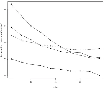
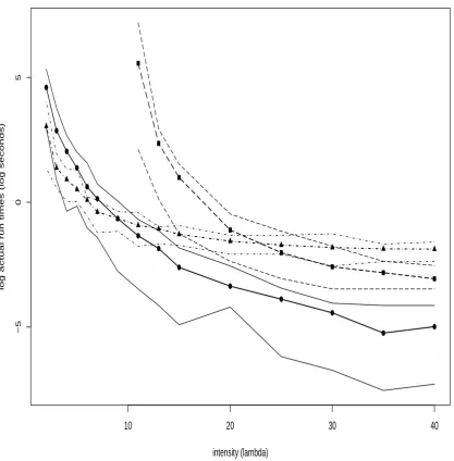
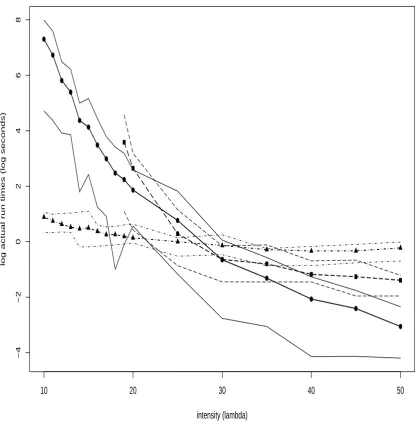
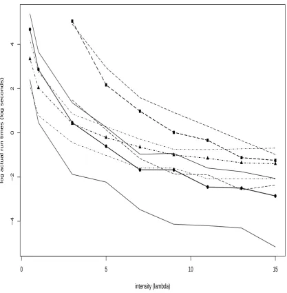
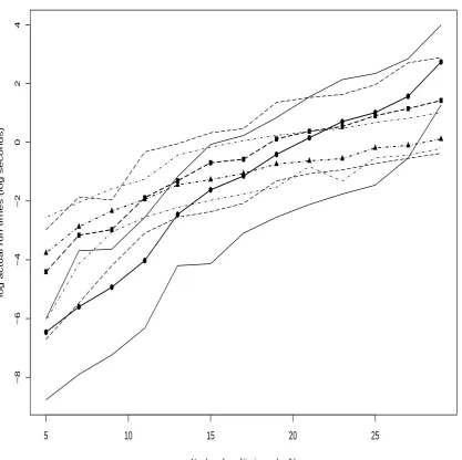
3.7.3 Experiment 1: Run Times Versus Intensityλ . . . 84
3.8 Conclusions & Further Work . . . 91
Chapter 4 Area-Interaction Point Process 93 4.1 Introduction . . . 93
4.2 Definition of the Area-Interaction Process . . . 95
4.2.1 Boundary Conditions . . . 96
4.3 Rejection Sampling . . . 96
4.4 Gibbs Sampling . . . 98
4.4.1 Attractive Case . . . 99
4.4.2 Repulsive Case . . . 99
4.4.3 Exact Gibbs: Attractive Case . . . 100
4.5 Simulation via Spatial Birth-Death Processes . . . 101
4.5.1 The Free Process . . . 103
4.5.2 The Interacting Process . . . 105
4.5.3 Simulation ofΨ: Time Stationary Construction . . . 107
4.5.4 domCFTP: Attractive Area-Interaction . . . 108
4.5.5 Clan Algorithm . . . 111
4.5.6 A Space-Time Percolation Problem . . . 114
4.6 Omnithermal Sampling . . . 115
4.6.1 Computing the Omnithermal Threshold . . . 118
4.6.2 The Omnithermal Process . . . 120
4.6.3 Finite Time Construction . . . 121
4.6.4 Time Stationary Construction . . . 123
4.7 Conclusions & Further Work . . . 124
4.7.1 Perfection in Space . . . 124
4.7.2 Omnithermal Sampling . . . 125
Chapter 5 Conditional Area-Interaction Point Process 127 5.1 Introduction . . . 127
5.2 Notation . . . 128
5.4 Simulation via Spatial Birth-Death Processes . . . 130
5.4.1 domCFTP: Conditional Area-Interaction . . . 131
5.5 Gibbs Sampling . . . 136
5.5.1 Exact Gibbs: Attractive Case . . . 139
5.5.2 Exact Gibbs: Repulsive Case . . . 144
5.6 Implementational Issues . . . 145
5.6.1 Large Sampling Window . . . 145
5.6.2 Implementation via 2-Stage Procedure . . . 146
5.7 Simulation Results . . . 146
5.7.1 Experiment 1: Run Times Versus Intensityλ . . . 147
5.7.2 Experiment 2: Run Times Versus Intensity Window Size . . . 148
5.7.3 Experiment 3: Run Times Versus Interaction Parameterβ . . . 152
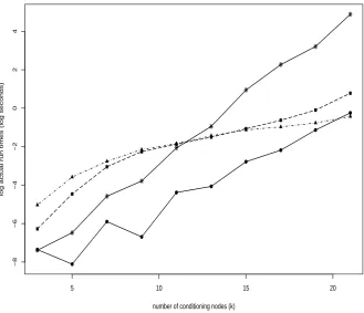
5.7.4 Experiment 4: Run Times Versusk . . . 152
5.8 Conclusions & Further Work . . . 156
5.8.1 Omnithermal Sampling . . . 156
5.8.2 Bayesian Cluster Modelling . . . 156
Chapter 6 Conclusions & Further Work 159 6.1 Further Work: Omnithermal Sampling . . . 160
Appendix A χ2 Tests: Conditional Boolean Model 163
Appendix B χ2 Tests: Conditional Area-Interaction 169
Bibliography 175
List of Figures
1 Redwood Seedlings . . . xvi
1.1 domCFTP . . . 33
3.1 Conditional Boolean Model . . . 63
3.2 Maximum Clique Size . . . 81
3.3 Run Times Versusλ . . . 82
3.4 Run Times Versusk . . . 83
3.5 Run Times Versusλ . . . 85
3.6 Run Times Versusλ . . . 86
3.7 Run Times Versusλ . . . 87
3.8 Run Times Versusk . . . 89
3.9 Run Times Versusk . . . 90
4.1 Area-Interaction Process . . . 97
4.2 The ‘Cluster’ Trick . . . 106
4.3 Clan Construction . . . 113
4.4 Computing the Omnithermal Threshold . . . 121
5.1 Conditional Area-Interaction Process . . . 129
5.2 Run Times Versusλ . . . 149
5.3 Run Times Versusλ . . . 150
5.4 Run Times Versus Window Size . . . 151
5.5 Run Times Versusβ . . . 153
5.7 Run Times Versusk . . . 155 5.8 Bayesian Cluster Modelling . . . 158
List of Tables
A.1 χ2 Tests: Conditional Boolean Model . . . . 165
A.2 χ2 Tests: Conditional Boolean Model . . . . 166
A.3 χ2 Tests: Conditional Boolean Model . . . 167
A.4 χ2 Tests: Conditional Boolean Model . . . . 168
B.1 χ2 Tests: Conditional Area-Interaction . . . . 170
B.2 χ2 Tests: Conditional Area-Interaction . . . 171
B.3 χ2 Tests: Conditional Area-Interaction . . . . 172
Acknowledgments
I would like to thank my supervisor Professor Wilfrid S. Kendall for his continued help and guidance throughout my Ph.D. This thesis was funded by an EPSRC studentship (No. 0080183X) and I gratefully acknowledge the financial support. Finally, to my parents and brother for their continued love and support.
Declarations
I declare that this thesis is based on my own research and in accordance with the regulations of the University of Warwick. The work is original except where indicated by specific references in the text. Chapter 2 is based on the following research report and subsequent publication:
Shah S.R. (2003). Stochastic domination and conditional thinning in spatial point processes. Technical Report 412, University of Warwick, UK.
Shah S.R. (2003). A note on stochastic domination and conditional thinning. Advances in Applied Probability (SGSA)5(4), 937–940.
Abstract
This thesis is about probabilistic simulation techniques. Specifically we consider theexactorperfect
sampling of spatial point process models via the dominated CFTP protocol. Fundamental among point process models is the Poisson process, which formalises the notion of complete spatial ran-domness; synonymous with the Poisson process is the Boolean model. The models treated here are the conditional Boolean model and the area-interaction process. The latter is obtained by weighting a Poisson process according to the area of its associated Boolean model.
A fundamental tool employed in the perfect simulation of point processes are spatial birth-death processes. Perfect sampling algorithms for the conditional Boolean and area-interaction models are described. Birth-death processes are also employed in order to develop an exactomnithermal algo-rithm for the area-interaction process. This enables the simultaneous sampling of the process for a whole range of parameter values using a single realization. A variant of Rejection sampling, namely 2-Stage Rejection, and exact Gibbs samplers for the conditional Boolean and area-interaction pro-cesses are also developed here.
Introduction
The huge increase in computing power over the last 25 years has had a profound effect on statistical methodology and applied probabilistic modelling. There have been numerous developments and application of simulation methods in various fields. Realistic models for real-world phenomenon usually involve a wide variety of complexity on high (or even infinite) dimensional state spaces. Mathematical analysis of such models is therefore difficult, if not impossible. However the onset of ever more powerful computers has made it possible to examine such models viastochastic simula-tion: (stochastic) realizations of the models can be obtained and statistical analysis carried out. This has spurred a whole new generation of stochastic simulation algorithms; one in particular, Markov Chain Monte Carlo (MCMC), is now widely used and recognized as a powerful tool in the statis-tics community. Its origins can be traced back to statistical physics (Metropolis et al. 1953), and concerns the simulation of models via Markov chains or processes.
The essence of MCMC involves the construction of a Markov chain whichconvergesto a stochas-tic realization of the model being studied. This class of algorithms has had numerous applications in statistical physics, image analysis, Bayesian statistics and, more recently, spatial modelling and stochastic geometry. However there is a basic set back with MCMC: in practice one has to settle for
approximatesamples, since a priori it is difficult in most cases to determine when the Markov chain will have converged. However it has been discovered that, for some chains, it is possible to modify the MCMC algorithm such that it automatically signals when convergence has been achieved.Such variants, which deliverexactsamples, have been coinedperfectorexact simulationalgorithms.
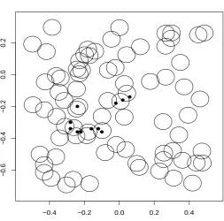
1995), concerns the modelling of phenomena that arise as complicated geometrical shapes or pat-terns. Furthermore, point processes provide plausible models for collections of individuals or events, such as plants, animals, stars, structure of biological cells and rock sections, disease outbreaks and earthquakes. For example Figure 1 below depicts the locations of the Redwood seedlings data which was originally studied by Strauss (1975), and later by Ripley (1977). It is clear from the figure that there is an underlying ‘clustering’ mechanism generating this data. Therefore a natural way to model these seedlings would be to assume that there is anunobserved ‘parent’ processwhich gives rise to theobserved ‘daughter’ process. The objective then would be to sample the parent process given
the observed daughter process.
0.0 0.2 0.4 0.6 0.8 1.0
0.0
0.2
0.4
0.6
0.8
1.0
[image:17.595.160.420.301.556.2]Redwood Seedlings
Figure 1:Positions of the Redwood seedlings; the data was obtained by kind permission from Peter Diggle’s web page
http://www.maths.lancs.ac.uk/˜diggle/.
Perfect simulation has developed rapidly since its inception. For example Coupling From The Past (CFTP)is probably the most popular and widely studied perfect simulation algorithm. It was introduced by Propp & Wilson (1996) for Markov chains on finite state spaces. Within the next few years it was generalized to continuous and even unbounded state spaces (Murdoch & Green 1998; Kendall 1998; Häggströmet al. 1999; Kendall & Thönnes 1999; Green & Murdoch 1999; Kendall & Møller 2000; Berthelsen & Møller 2002b). It has also been the focus of several doctoral
theses (Wilson 1996; Thönnes 1998; Dimakos 2000; Ambler 2002). While providing solutions to problems of convergence and approximates samples, it also poses more challenges to the researcher. This thesis is another addition to the simulation literature, aiming to introduce and develop more perfect simulation algorithms for point processes.
Overview of Thesis
This thesis comprises five main chapters, a concluding chapter and two appendices. We consider the perfect sampling of the conditional Boolean model, area-interaction and conditional area-interaction process. An investigation of the Van Lieshout & Van Zwet (2001) algorithm for conditional Boolean models, which concludes that their method is actually biased, is first presented. Following this three perfect sampling procedures for the conditional Boolean and conditional area-interaction models are described: a 2-Stage Rejection method, one employing spatial birth-death processes and an exact Gibbs sampler. For the area-interaction process, several existing algorithms are reviewed and the possibility ofomnithermalsampling for the process is also considered.
The basic theory and foundations for point processes and their simulation is introduced in Chap-ter 1. A natural way to sample point processes is via spatial birth-death processes, introduced by Preston (1977); indeed a number of CFTP-based perfect algorithms employ birth-death processes (Kendall 1998; Kendall & Thönnes 1999; Berthelsen & Møller 2002b; Fernándezet al. 2002). A description of how point processes can be simulated via spatial birth-death processes is given and il-lustrated by simple examples. Chapter 1 also introduces the ideas behind Markov Chain Monte Carlo (MCMC) and perfect simulation, including a description of the Coupling From The Past (CFTP) and Dominated CFTP (domCFTP) protocols.
to the case ofstrictstochastic dominance (Corollary 2.1). This allows the bias of the Van Lieshout & Van Zwet algorithm to be quantified in some cases.
Chapter 3 then considers various other perfect simulation algorithms for conditional point pro-cesses. A 2-Stage Rejection algorithm is developed and shown to be more efficient than ordinary Re-jection. The Cai & Kendall (2002) algorithm is described in Section 3.4.1. The original formulation employs immigration-death processes on the integers; the description here is phrased, equivalently, in terms of spatial birth-death processes. Gibbs sampling for conditional point processes has not been considered before in the literature; therefore Section 3.5 describes a CFTP-based Gibbs sam-pler. The coupling construction vaguely resembles that of Häggströmet al. (1999), as their notion ofquasi-minimalandquasi-maximalelements is employed in order to devise the required coupling of ‘bounding’ processes. Results of simulation experiments, aimed at comparing the performance of the 2-Stage Rejection, Cai & Kendall and exact Gibbs algorithms, are presented in Section 3.7. The basic conclusion is that 2-Stage Rejection is very competitive for moderate parameter values, whereas the Cai & Kendall algorithm performs well for extreme values. The exact Gibbs sampler, unfortunately, is always outperformed.
The area-interaction process of Baddeley & Van Lieshout (1995) is the focus of Chapter 4. Rejec-tion, Gibbs sampling and two methods (Kendall 1998; Fernándezet al. 2002), which use birth-death processes, are reviewed. Simulation via spatial birth-death processes involves computation of areas of irregular regions in order to determine appropriate acceptance probabilities. Here, we develop the ‘cluster’ trick of Kendall (1997a), yielding the first implementation of the Kendall (1998) algorithm which employs this trick. The algorithms considered so far sample the area-interaction process for
fixedmodel parameters. The emphasis in Section 4.6 is onomnithermal sampling, where the pro-cess is sampled for a whole rangeof parameter values simultaneously (cf. Propp & Wilson 1996 and the references therein, Wilson 1996, Dimakos 2000 and Grimmett 1995). The area-interaction process has not been the study of such a sampling procedure; the work here has yielded an exact omnithermal algorithm for this point process.
Chapter 5 combines the ideas of Chapters 3 & 4 and introduces the ‘conditional area-interaction process’. We incorporate the Cai & Kendall (2002) and Kendall (1998) algorithms in order to define a domCFTP construction. In addition a 2-Stage Rejection procedure and an exact Gibbs-within-Metropolis Hastings sampler are also developed. A quantitative evaluation of the actual run
times of these three procedures is carried out. The results indicate that the modified Cai & Kendall algorithm performs well for extreme model parameters, while the 2-Stage and Gibbs algorithms are competitive for moderate parameter values. It is not the case now that the Gibbs sampler is always outperformed by the other two; it is as efficient, if not more so, than the 2-Stage algorithm for all parameter values.
Chapter 1
Mathematical Foundations
1.1
Stochastic Geometry & Point Processes
Stochastic Geometry refers to that area of Mathematical research which provides suitable models and statistical methods for analyzing data representing complicated geometrical patterns. Examples of such patterns include the (spatial) distribution of stars and galaxies, locations of trees in a forest, features of biological tissues, rock sections studied in geology, oil reservoirs and ore deposits. The modern theory of Stochastic Geometry was initiated by D.G. Kendall, K. Krickeberg and R.E. Miles (see Stoyanet al.1995 for a variety of literature on the historical origins and recent advances; D.G. Kendall’s foreword provides an anecdotal glimpse into the origins of the subject).
The most basic geometrical objects are points, and collections of random point patterns or ‘point processes’ play a fundamental role in stochastic geometry. More complicated objects can be built from a collection of points, eg. the Boolean model (Definition 1.10 or 3.1); in addition the theory of line and surface processes generalizes the notion of point patterns to higher dimensions and is useful for modelling applications in geology, stereology and medicine (a rigorous treatment is given in Stoyanet al.1995). The main aim of this thesis is to present new and existing simulation algorithms for some point process models.
A spatial point pattern on some space X can be viewed as a finiteunordered set or ‘configura-tion’ of points x = {ξ1, . . . , ξn} for n ∈ N, ξi ∈ X. Point patterns modelling different physical
either ‘points’ or ‘individuals’. Point processes can also be viewed as random counting measures or random variables taking values in what is called anExponential Space(Carter & Prenter 1972). Rigorous theoretical treatments of point processes have predominantly been made in terms of the random measure viewpoint (see for example Daley & Vere-Jones 1988, 2003). On the other hand, it is much more convenient to adopt the random variable viewpoint when considering simulation algorithms for point processes (Stoyanet al. 1995; Van Lieshout 2000; Møller 1999; Geyer 1999; Ripley 1977). The treatment via random variables or unordered sequences/sets of points arises more naturally when modelling interactions between the individuals.
1.1.1
Point Processes & Exponential Spaces
Let X be a complete separable metric space (c.s.m.s.). As noted in the previous section a point processX onX can be thought of as a random set or unordered sequence of points or individuals
{ξn}, ie. X is a random variable taking values in the Exponential Space of X, denoted by Xe
(Carter & Prenter 1972). Informally speaking, Xe is the space of all finite (Definition 1.2) point
configurations onX. A formal interpretation and construction of Xe is given in Preston (1977): let
Xn denote the n-fold product ofX. Identify those points of Xn which can be obtained from each
other by permutation of the co-ordinates and denote the space obtained by this identification asSn.
SettingXe = UnSn (where the Sn are disjoint) gives us the Exponential Space ofX. LetB(X)
denote the Borelσ-algebra on X, B(Sn)the product σ-algebra generated by open sets ofSn and
B(Xe) theσ-algebra generated by theB(Sn). A point process X on some bounded W ⊆ X can
hence be defined as anWe-valued random variable:
Definition 1.1. Apoint processX on some boundedW ⊆ X is a measurable mapping of a proba-bility space(Ω,=,P)to(We,B(We)).
For a point processX andA∈ B(Xe)letX(A)be the number of points ofX inA. Implicit in the
above definition is thatX is finite or locally finite.
Definition 1.2. A point processX isfiniteifX(X)<∞.
Definition 1.3. X islocally finiteifX(A)<∞for all boundedA∈ B(X). Definition 1.4. X issimpleifX({ξ}) = 0or1for allξ ∈ X.
1.1.2
Point Processes & Random Measures
In this section we follow the treatment of point processes as random counting measures, as presented in Daley & Vere-Jones (1988, 2003) and Stoyanet al. (1995). For a point process X = {ξn}and
A∈ B(X)the mappingX(A) = #{n; ξn ∈A}counts the number of points ofXcontained inA.
IfA=S
nAn, with theAndisjoint, thenX(A) =
P
nX(An)is a countably additive, non-negative,
integer-valued function withX(A) < ∞for all boundedA. These are exactly the conditions that makeX(·)countingmeasure (ie. a non-negative integer-valued measure) on B(X). A measureµ
onX is boundedly finite ifµ(A) < ∞ for all bounded Borel setsA. Let MX be the space of all boundedly finite measures onX andB(MX)its corresponding Borelσ-algebra.
Definition 1.5. A random measure Y on X is a random element of (MX,B(MX)), ie. Y is a measurable mapping of a probability space(Ω,=,P)to(MX,B(MX)).
Acounting measureis a boundedly finite and integer-valued measure. Acompletely random mea-sure is a random measure Y such that, for every family of pairwise disjoint bounded Borel sets
A1, . . . , An, the random variablesY (A1), . . . , Y (An)are independent. Simple counting measures
are such thatY ({ξ}) = 0or1for allξ ∈ X. LetNX denote the space of counting measures onX,
B(NX)its correspondingσ-algebra andN∗X the space of simple counting measures onX, ie. N∗X constitutes those members ofNX which are simple.
Definition 1.6. Apoint processX onX is a measurable mapping of a probability space(Ω,=,P)
to(NX,B(NX)). Furthermore,X is simple ifP[X ∈N∗X] = 1.
“A measurable mapping X from a probability space into NX (or N∗X) is a point process if and only ifX(A) is a random variable for each Borel setA ⊆ X” (Daley & Vere-Jones 1988, Propo-sition 7.1.VIII). A point process X is a random choice of one of the elements of NX; so it gen-erates a measure P on (NX,B(NX)): the distribution of X, defined by P(B) = P[X ∈B] = P[{ω; X(ω)∈B}], for B ∈ B(NX). For x ∈ Xe, A ∈ B(X) let N(A, x) = x(A) =
P
Definition 1.7. Thefinite-dimensional (fidi) distributionsof a point processX are the joint distri-butions of the random variablesX(A1), . . . , X(Ak), for all finite collections of bounded Borel sets
A1, . . . , Ak, ie. the family of proper distribution functions
Pk(A1, . . . , Ak; n1, . . . , nk) =P[X(Ai) =ni, i= 1, . . . , k]. (1.1)
Definition 1.8. Thevoid probability(Stoyanet al. 1995) or theavoidance function(Daley & Vere-Jones 1988) of a point processX gives the probability that there are no points of the process in a given test setA: v0(A)≡P[X(A) = 0].
“The distribution of a point process is completely specified by the fidi distribution ofX(A)forAin a countable ring generating the Borel sets” (Daley & Vere-Jones 1988, circa Theorem 7.1.XI). More-over for simple point processes the distribution is determined by the void probabilities/avoidance functionv0 on compact sets (Stoyanet al.1995; Daley & Vere-Jones 1988, Theorem 7.3.II).
1.1.3
Characteristics of Point Processes
1. Stationarity & Isotropy: A point processX or its distributionPisstationaryif the processes
X = {ξn}andXξ = {ξn+ξ}have the same distributions for allξ ∈ X, ie. the distribution
is translation invariant: P(B) ≡ P[X ∈B] = P[Xξ ∈B] ≡ P(B−ξ)for all B ∈ B(NX), where Bξ = {Y ∈NX; Y−ξ ∈B}. The process isisotropicif it is rotation invariant: ifris
a rotation around the origin thenX andrX have the same distribution, ie. P(B) =P(rB)
for all B ∈ B(NX), where rB = {Y ∈NX; r−1Y ∈B}. Stationarity and isotropy imply motion invariance: the distribution ofXis the same asmX for all Euclidean motionsm.
2. Intensity Measure: The intensity measureΛofX is a characteristic analogous to the mean of a real-valued random variable. It is defined as the mean number of points inA∈ B(X):
Λ (A) =E[X(A)] =
Z
x(A)P(dx).
ForX =Rd, ifX is translation invariant thenΛ (A) =λ m
d[A]wheremddenotes Lebesgue
measure andλ >0is referred to as theintensityofX. ChoosingAto haved-volume1shows that λ may be interpreted as the mean number of points per unit d-volume. The Campbell
Theorem(Stoyanet al.1995) shows that for any non-negative measurable functionf:
E
" X
ξ∈X
f(ξ)
#
=
Z X
ξ∈x
f(ξ)P(dx) =
Z Z
f(ξ)x(dξ)P(dx) =
Z
f(ξ) Λ (dξ) ;
and for stationaryX : E
" X
ξ∈X
f(ξ)
#
=λ
Z
f(ξ)dξ.
1.1.4
Construction of Point Processes
A convenient and constructive way to model and simulate point processes on bounded regions is by means of a “discrete distribution for the number of points and a family of symmetric densities for the locations” (Van Lieshout 2000; Daley & Vere-Jones 1988, Condition 5.3.I):
• The points are located in a complete separable metric space (c.s.m.s.)X, such asRd.
• A distribution{pn}n≥0 is given for determining the total number of points in the population.
• For each integer n ≥ 1, a symmetric probability density fn(ξ1, . . . , ξn) is given that
deter-mines the joint distribution of the positions of thenpoints of the process.
This provides a natural recipe for simulating a point process: first simulate the number of points
N according to the distribution {pn}; given that N = n generate a random vector (ξ1, . . . , ξn)
according to the density fn(·, . . . ,·). As noted in Daley & Vere-Jones (1988), point processes are
unordered sets or sequences of points; therefore it is implicitly assumed that the individuals of the process are indistinguishable. So the joint densitiesfnshould be indifferent to the order in which the
points are listed, ie. they have to besymmetricso that equal weight is given to alln!permutations of the points(ξ1, . . . , ξn).
1.1.5
The Poisson Process
This is mathematically the most-tractable and perhaps the most studied point process (Matheron 1975; Diggle 1983; Ripley 1981; Ripley 1988; Daley & Vere-Jones 1988; Kingman 1993; Stoyan
Definition 1.9. LetX be a c.s.m.s. andΛa Borel measure such thatΛ (X)>0andΛ (A)<∞for all bounded BorelA;X is aPoisson processwith intensity measureΛif
P1 X(A)is a Poisson random variable with meanΛ (A)for every bounded Borel setA⊆ X;
P2 for all disjoint BorelA1, . . . , Ak, the random variablesX(A1), . . . , X(Ak)are independent.
IfΛis atom-less (ie. gives zero measure to singleton sets) then the Poisson process is simple (Def-inition 1.4). P2is often interpreted ascomplete spatial randomness: the process in disjoint regions behaves independently. IfX =RdandΛ (A) =λ m
d[A](cf. Section 1.1.3), formdLebesgue
mea-sure, thenXis referred to as ahomogeneous Poisson processwith intensityλ >0, and abbreviated asX ∼Poisson(λ). In order to simulate a Poisson(λ)process onW ⊂Rd: draw a Poisson random
variable N with mean λmd[W]. IfN = 0 setX = ∅; else for each n ∈ {1, . . . , N} drawξn ∼
Uniform(W)and setX ={ξ1, . . . , ξN}.
AninhomogeneousPoisson processX0 is one whose intensity measure is of the formΛ0(A) =
R
Aλ
0(x)dx. The function λ0(·) is referred to as the intensity function. The following rejection technique enables one to draw X0. Draw X ∼ Poisson(λ) such that λ0(·) ≤ λ; then X0 =
n
ξ∈X; λ0λ(ξ) ≤ Uniform(0,1)o, ie. each point of X is retained with probability λ0λ(·) to yield an inhomogeneous Poisson process with intensity functionλ0(·). One can also construct random geometrical shapes/patterns via Poisson processes by defining the Boolean model (Stoyan et al.
1995) of disks of fixed radiusr.
Definition 1.10. LetX = {ξn}be a Poisson(λ)process onRd andBr(ξ)ad-dimensional ball of
radiusrand centreξ. Then theBoolean modelof balls associated withXis constructed as
U(X) = [
n≥1
Br(ξn). (1.2)
The points ofX are called germs and the ballsBr(·)grains; thus the Boolean model can also be
viewed as agerm-grain random set model.
A more general definition of Boolean models is given in Chapter 3 (Definition 3.1). However the basic idea of such models is introduced here since Chapter 2 concerns the simulation of conditional Boolean models.
1.1.6
Finite Point Processes Specified by a Density
Poisson processes are a useful tool for building more complex point process models, eg. thePoisson cluster process, which is obtained by independently replacing each point of a Poisson process by a finite ‘daughter’ process. Special cases are theNeyman & Scott (1958) process, where the daugh-ters are independent and identically distributed, and theMatérn (1986) cluster process, where each parent gives rise to a Poisson number of daughters distributed in a ball of radiusraround the parent. Other useful point process models can be obtained by specifying a density with respect to a ‘reference’ Poisson process. Letπdenote the distribution of a Poisson process onX with intensity measureΛ, andf : Xe → [0,∞) be a non-negative measurable function on the exponential space
(space of locally finite point configurations) Xe. If
R
Xef(x)π(dx) = 1 then f is a density with respect to π and defines a point process Xf on X. Thus, given a reference process X (usually
Poisson(1)) with distributionπ, a new processXf ∼ πf can be defined on (Xe,B(Xe))by means
of a density f such that πf =
R
f(x)π(dx). Then f(x) is the likelihood that Xf takes on the
realizationx compared with X taking on the same realization. The distribution of the number of points in the new processXf specified by densityf is given by
pn =
e−Λ(X)
n!
Z
X
. . .
Z
X
f({ξ1, . . . , ξn}) Λ (dξ1). . .Λ (dξn)
(Van Lieshout 2000). Conditional on the event thatXf hasnpoints, the density (with respect to the
n-fold product measureΛn) of the locations of the points is given by
fn(ξ1, . . . , ξn) =
f({ξ1, . . . , ξn})
R
X. . .
R
X f({ξ1, . . . , ξn}) Λ (dξ1). . .Λ (dξn)
.
Example 1.1 (The density of a Poisson process). LetX be a Poisson process onRdwith intensity measureΛand distributionπ. Letfλ(x) = λn(x) e(1−λ), wheren(x)denotes the number of points
inx, andπλ(B) =
R
Bfλ(x)π(dx)forB ∈ B(Xe). Thenπλis the distribution of a Poisson process
with intensity measureλΛand densityfλ.
Definition 1.11. A point process with densityf islocally stableif there existsK >0such that
f(x∪ {ξ})≤Kf(x), for allx∈ Xeandξ /∈x. (1.3)
The density is said to beRuelle (1969) stableiff(x)≤ CKn(x)for some positive constantsC, K.
Definition 1.12. A density is hereditary if f(x) > 0 ⇒ f(y) > 0 for y ⊂ x; conversely f is
anti-hereditaryiff(y)>0⇒f(x)>0fory⊂x.
1.1.7
Marked Point Processes
Suppose that, given the locations of objects or individuals, one wishes to not only model the spa-tial distribution but also some characteristic of each individual, eg. the diameter or height of trees, shape, colour, weight of animals, etc. Such information can be modelled bymarked point processes: to each point or individual of the process a ‘mark’ is attached which represents the feature or char-acteristic. Thus a marked processX on some spaceX is a random unordered sequence of tuples
X = {(ξn, mn)} such that the {ξn} themselves form a point process on X and mn is the mark
attached to the individualξn. The structure of the marks may be complicated and it is assumed that
they belong to a given space of marks M. A marked point process X on X can be viewed as a point process on the product spaceX ×M; all the theory of point processes extends to marked point processes (see for example Daley & Vere-Jones 1988 or Stoyanet al.1995).
Definition 1.13. A marked point processX, with positions inX and marks inM, is a point process onX × M with the additional property that{X(A×M) ; A∈ B(X)}, the marginal process of locations, is itself a point process.
1.1.8
Interior & Exterior Conditioning
The conditional distribution of a point processX can be defined under two types of conditioning:
Exterior: This type of conditioning concerns the conditional distribution of the point process at someξ ∈ X given the configuration onX \ {ξ}, ie. the (conditional) probability that there is a point in an infinitesimally small regiondξaroundξ, given the configuration outsidedξ.
Interior: This concerns the conditional distribution of the process onX \ {ξ}, given a point atξ.
“The two concepts are dual; exterior conditioning is formalized by the Papangelou conditional intensity, interior conditioning by the Palm distribution” (Van Lieshout 2000). The Papangelou conditional intensity was introduced by Papangelou (1974) and Palm distributions by Palm (1943).
Palm Distributions
For a point processX with distributionPa heuristic interpretation of the Palm distribution, Pξ, is
the conditional distribution ofXgiven thatX({ξ})> 0, ie. palm probabilities are the conditional probabilities ofX given that there is a point at locationξ. For a more rigorous definition, one needs the concept ofCampbell measures(Stoyanet al.1995):
Definition 1.14. IfXis a simple locally finite point process on a c.s.m.s. X with distributionPthen itsCampbell measureis the measure on(X × Xe,B(X)× B(Xe))such that
Z X
ξ∈x
f(ξ, x)P(dx) =
Z
f(ξ, x)C(d(ξ, x)) (1.4)
wheref is any non-negative measurable function onX × Xe. Iff(ξ, x) = 1{ξ∈A} andA ∈ B(X) thenC(A×B) = EX(A)1{X∈B}
, forB ∈ B(Xe).
Definition 1.15. TheReduced CampbellmeasureC!is such that
Z X
ξ∈x
f(ξ, x\ {ξ})P(dx) =
Z
f(ξ, x\ {ξ})C!(d(ξ, x)) (1.5)
Moreover,C!(A×B) =
E
h P
ξ∈X∩A1{X\{ξ}∈B}
i .
If the intensity measure Λ ofX exists then C(· ×B) is absolutely continuous with respect to Λ, with Radon-Nikodym derivativeP·(B) :X →R, so that
C(A×B) =
Z
A
Pξ(B) Λ (dξ), for allA∈ B(X). (1.6)
For fixedξ,Pξ is a distribution function on(Xe,B(Xe))and is referred to as thePalm distribution
atξ. Similarly thereduced Palm distributionP!
ξis related toC!via
C!(A×B) =
Z
A
P!ξ(B) Λ (dξ) (1.7)
soP!
0(B) = P[X\ {0} ∈B |0]is the conditional distribution ofX\ {0}given thatX({0})>0.
Papangelou Conditional Intensities
Turning attention to the dual case of exterior conditioning the Papangelou conditional intensity `
associated with a simple point processXcan be interpreted as
the “infinitesimal probability that there is a point in a regiondξ aroundξ ∈ X given that the point processX agrees with the configuration xoutside dξ” (Van Lieshout 2000). A more formal def-inition requires the concept of the reduced Campbell measure C! (Definition 1.15). The reduced Palm distribution (Eq. 1.7) is the Radon-Nikodym derivative of C!(· ×B) with respect to the
in-tensity measureΛof the point processX. IfC!(A× ·)is absolutely continuous with respect to the
distributionPofX then
C!(A×B) =
Z
B
L(A;x)P(dx), A∈ B(X) (1.8)
for some measurable function L(·;x), which is referred to as the first order Papangelou kernel. Furthermore ifL(·;x)admits a density`(·;x)with respect to the intensity measure Λ ofX, then
`(·;·)is called the (first order) Papangelou conditional intensity. When X admits a density with respect to a Poisson process the Papangelou conditional intensity takes a simple form, and provides a useful way to simulate such processesX(cf. Section 1.3.2).
Theorem 1.1 (Van Lieshout 2000, Theorem 1.6). For X a finite process specified by density f
with respect to a Poisson process the Papangelou conditional intensity is given as
`(ξ;x) = f(x∪ {ξ})
f(x) , forξ /∈x∈ Xe (1.9)
with convention that`(ξ;x) = 0iff(x) = 0.
Suppose that a point processX has density f with respect to a Poisson(λ) process, and recall the notions of local stability and hereditary density (Definitions 1.11 & 1.12). The densityf is locally stable if there exists a constantK >0such thatf(x∪ {ξ})≤ Kf(x)for allxand allξ /∈ x; it is hereditary iff(x)>0 ⇒f(y)>0fory ⊂x. It is clear that a locally stable density is hereditary. Furthermore if the Papangelou conditional intensity of f, defined as in Eq. (1.9), is uniformly bounded then local stability and the hereditary condition are equivalent (Kendall & Møller 2000). The densityf may also beattractiveorrepulsive:
attractive: `(ξ;x)≥`(ξ;y), wheneverξ /∈y⊆x; (1.10)
repulsive: `(ξ;x)≤`(ξ;y), wheneverξ /∈y⊆x. (1.11)
1.1.9
Operations on Point processes
In this section three fundamental operations on point processes are presented which produce new processes from old ones. Denote by X0 the basic or reference process to which the operation is
carried out on andX the new process so obtained.
Thinning: Such a operation uses some criterion to delete points of the basic processX0 and yield
a thinned process X. The simplest thinning operation is an independent p-thinning, where each ξ ∈ X0 is deleted with probability 1 − p, for some p ∈ [0,1]. Deletion of a point
is independent of its location and of other points in X0. An extension of this is to allow
the retention probability p to depend on the location of the point; thus ξ ∈ X0 is deleted
with probabilityp(ξ), for some deterministic (or even random) function p(·)defined on X, and taking values in [0,1]. One could also define dependent thinnings where the retention probability depends on the locations of other points as well.
In the case of independent thinning, if the characteristics of the basic processX0 are known
then it is straightforward to calculate the corresponding characteristics of the thinned process
X. IfX0is a Poisson process with intensity measureΛ0 then an independentp(·)-thinning of
X0 is also a Poisson process, with intensity measureΛ (A) =
R
Ap(ξ) Λ0(dξ).
Clustering: In this case every pointξof the basic processX0 is replaced by a clusterYξ of points.
X0 is referred to as the parentprocess and Yξ the daughterprocess. The unionSξYξ is the
clusterprocess, with the daughtersYξthemselves being finite point processes.
Such processes have been used to model many natural phenomenon, eg. locations of galax-ies in space, distribution of larvae in fields, the geometry of bombing (cf. Figure 1). If the daughters Yξ are independent identically distributed finite point sets then this is called
ho-mogeneous independent clustering; moreover if the parent process X0 is Poisson then the
resulting daughter process is aPoisson cluster process. Important cases are the Neyman & Scott (1958) model, where daughters are independent and identically distributed; and Matérn (1986) cluster process, where daughters are distributed in a ball of radiusraround the parent. Superposition: Here a collection of basic processes{Xi
0}
k
i=1are combined to form a single process
X =Sk
i=1X
i
super-imposed processXis just the sum of the intensity measures of the basic processes. If{X0i}ki=1
are independent Poisson processes (not necessarily with the same intensity measures) thenX
is also a Poisson process.
1.1.10
Gibbs Point Processes
There are many different classes or models of point processes that have arisen in the literature over the years and this section considers the class referred to as Gibbs point processes. They are a development of the idea in Section 1.1.6: that new point processes can be obtained from old ones by transforming their distributions via a probability density. Following Daley & Vere-Jones (1988) and Stoyanet al.(1995) the construction of Gibbs processes is described below. The origins of such processes stem from statistical physics, being related to the so-calledGibbs distributions
which describe the equilibrium states of subsystems of very large closed physical systems. Such processes are described by means of forces acting on and between the particles. The total potential energy of a given configuration of particles or individuals is assumed to be decomposable into terms representing the interactions between the particles taken in pairs, triples, and so on. First-order terms representing the presence of an external force can also be included. Thus Gibbs processes can be thought of as processes generated byinteraction potentials.
The fundamental ingredient in specifying a Gibbs process X is an underlying basic or weight
processX0 with distributionQ(this is usually taken to be a Poisson process). The distributionPof
a Gibbs process can then be defined by means of a densityf:
P(B) =
Z
B
f(x)Q(dx), B ∈ B(Xe). (1.12)
Rather than specifying a distributionPfor the Gibbs process and then checking absolute continuity PQ, the usual trick is to do the reverse. An integrable functionf (with respect toQ) is specified and the distribution P is then defined via Eq. (1.12). The form of f is often determined by the field of application: it can be chosen conveniently to model interactions between individuals of the process. This approach is straightforward if the process contains only finitely many points confined to a bounded regionW. More generally, for point processes in all ofX, the density idea must be applied to conditional distributions confined to bounded regions.
Gibbs Processes in Bounded Regions
In this section we consider how to define Gibbs point processes in a bounded regionW ⊂ X. In order to do so there are two different cases to consider:
Canonical Ensemble: Here the process contains a fixed number n of particles, all contained in
W. This is of great practical importance since one often conditions on the number of points observed in someW. The form off is usuallyf(x) =f(ξ1, . . . , ξn) = e
−U(x)
Z , whereZ is a
normalizing constant called theconfigurational partition function, andU : Xe → R∪ {∞}
is the energy function. Frequently U is chosen to have a specialized form: an interaction potentialU(x) = P
y⊂xV (y); or a sum ofpair potentialsU(x) =
P P
1≤i,j≤nθ(kξi−ξjk).
The functionθ is referred to as the pair potential, in homage to the origins of the subject in Physics, andk · kis a norm onX.
Grand Canonical Ensemble: Here the total number of pointsN is random but all assumed to be within W. One approach is to define a sequence of “conditional densities” fn. The Gibbs
process is then obtained by first arrangingN to have some distribution and then (conditional on the value ofN) using the Canonical Ensemble construction. That is givenN = n then
points are distributed inW using the joint densityfn. Another approach is to define a density
directly onB(We), whereWeis the exponential space (Section 1.1.1) ofW.
Stationary Gibbs Processes
When considering Gibbs processes on unbounded spacesX, a more sophisticated method than just specifying the density on boundedW ⊂ X is required. Additionally, the distribution of the process restricted to the observation windowW must beconditionedon the process outsideW.
Formally one considers the family oflocal specificationsπW (· | ·)for bounded BorelW. These
represent the probability that the Gibbs processXonW belongs to the setB ∈ B(Xe), given that the
process takes on some configurationxoutsideW, ie.πW(B |x) = P[X∩W ∈B |X∩Wc=x],
wherex∈ {y∈ Xe; y(B) = 0}. Then a point processX with distributionPis said to be aGibbs
after Dobrushin, Lanford & Ruelle (Stoyanet al.1995), holds: DLR-Equation: P(B) =
Z
πW(B |x∩Wc)P(dx). (1.13)
Examples of Gibbs Point Processes
Any process with density of the form given in Canonical Ensemble is a Gibbs process; some exam-ples are given below and several more in Section 1.1.11, as examexam-ples of Markov point processes.
1. Hard Core Process: This is a process where no two points are allowed to be within distance
R > 0of each other, so that the density is given byf(x)∝λn(x)Q
{ξ,η:ξ6=η}1{kξ−ηk>2R}. 2. Strauss Process: This model has density with respect to a Poisson(1) given by f(x) ∝
λn(x)eβ sR(x). The parameter λ > 0 represents the underlying Poisson intensity and s
R(x)
denotes the number of pairs ξ, η ∈ xwhich are closer than distance R >0. This is an exam-ple of apair-wiseinteraction Gibbs process, since the density depends only on the number of
R-close pairs. The case when β = 0corresponds to a Poisson(λ)process; whenβ → −∞
the Strauss process converges to the hard core model since eβ sR(x) will be non-zero only if
sR(x) = 0. The Strauss process can be considered as asoft coreprocess since the density is
weighted by the number ofR-close pairs; the case when the weight is non-zero only for zero
R-close pairs corresponds to a hard core process.
3. Geyer (1999) remarks that in practical applications, “it is likely that no process model in the existing literature would be of scientific interest and a model specific to the application would be invented”. Furthermore, he illustrates the ease with which one can ‘invent’ new point processes and do statistical inference; the triplets andsaturation processes are described as examples of two new point processes.
1.1.11
Ripley-Kelly Markov Point Processes
These are another class of point processes, introduced by Ripley & Kelly (1977), and especially designed to model inter-point interactions. Let ∼ be a symmetric, reflexive relation on X, eg. if
X = Rd, thenξ ∼ η ⇔ kξ−ηk ≤ r for some fixedr. Two pointsξ, η are said to be neighbours
with respect to∼ifξ∼η.
Definition 1.16. Theneighbourhood∂W ofW ⊆ X with respect to the relation ‘∼’ is defined as
∂W ={ξ∈ X; ξ ∼ηfor someη∈W}.
Definition 1.17. LetX be a c.s.m.s.,Λa finite non-atomic Borel measure andπΛthe distribution of
a Poisson process onX with intensity measureΛ. LetXbe a point process onX specified by means of a densityf with respect toπΛ. ThenX is a(Ripley-Kelly) Markov point processwith respect to
the symmetric, reflexive relation∼onX if forx∈ B(Xe)such thatf(x)>0
1. f(y)>0for ally⊆x;
2. for allξ∈ X, f(xf∪{(x)ξ}) depends only onξand∂ξ∩x={η∈x; ξ∼η}.
Condition 2 above is alocal Markov property since it concerns the behaviour of at a single point; the followingspatial Markov propertyalso holds.
Theorem 1.2 (Ripley & Kelly 1977). LetX be a Markov point process with densityfon a c.s.m.s.
X and consider a Borel setW ⊆ X. Then the conditional distribution ofX∩W, givenX∩Wc,
de-pends only onXrestricted to the neighbourhood∂W∩Wc={ξ ∈ X \W; ξ∼ηfor someη∈W}.
Ripley & Kelly (1977) show that the density of a Markov point process is of the form
f(x) = 1
Z exp −
X
y⊂x
V (y)
!
, forx∈ Xe. (1.14)
HereV is aninteraction potential (cf. Section 1.1.10), so that V (x) 6= 0implies that y ∼ y0 for all y, y0 ⊂ x, for some relation ‘∼’. In graph-theoretic language V is non-zero for all cliques of
x. Further specializations of Markov point processes are Markov marked point processes, nearest-neighbour and connected-component Markov point processes (Van Lieshout 2000, Chapter 2).
Examples of Markov Point Processes
Such processes have been intensively studied as models for pair-wise (and possibly higher order) interactions (Van Lieshout 2000; Baddeley & Møller 1989; Ripley & Kelly 1977).
1. Hard/soft core processes.
3. Area/Perimeter/Quermass Interaction processes: The area-interaction process is a weighted Poisson process where the weight factor is a function of the area covered by the Boolean model (cf. Definition 1.10) associated with the process. The area-interaction process is stud-ied in Chapter 4. The perimeter-interaction process is a weighted Poisson process but with the weight depending on the perimeter of Boolean model. The quermass-interaction process (Kendallet al.1999) is such that the weight is determined by the area, perimeter and the Euler characteristic (cf. Stoyanet al.1995) of the Boolean model. The respective densities are:
area-interaction: f(x)∝λn(x)e−β1 m2[U(x)].
perimeter-interaction: f(x)∝λn(x)e−β2 p[U(x)].
quermass-interaction: f(x)∝λn(x)exp (β1m2[U(x)] +β2p[U(x)] +β3 χ[U(x)]).
Here m2, p, χ denote Lebesgue measure, perimeter length and Euler characteristic
respec-tively, andU(x)is the Boolean model associated withx. Notice that ifβ2 =β3 = 0then the
quermass-interaction process is just an area-interaction process.
4. Continuum Random Cluster model: Suppose ∼ denotes a relation where ξ ∼ η if U(ξ)∩ U(η) 6= ∅. Furthermore ξ and ξ0 are connected in x if there exist ξ0, . . . , ξn in x such that
ξ = ξ0 ∼ . . . ∼ ξn = ξ0. Such a connected component {ξ0, . . . , ξn} is called a cluster; let
the number of clusters in a point configuration xbeC(x). Settingf(x)∝λn(x)e−β C(x), for
λ >0, defines the continuum random cluster model (Møller 1999) with densityf.
5. Penetrable Spheres Model: This is a bivariate process obtained by conditioning two Poisson processes X1, X2 on the event that no point of one process is closer than a distance R > 0
to a point of the other. The process Y = (X1, X2)is called the Widom & Rowlinson (1970)
penetrable spheres model, with densityf(y) ∝ λn(x1)
1 λ
n(x2)
2 1{d(x1,x2)>R}, whered(x1, x2)is
the smallest distance between a point ofx1and a point ofx2.
1.2
Markov Processes
Consider a measurable space(X,B(X)), whereB(X)is the Borelσ-algebra onX. The aim of this thesis is to devise sampling schemes for point process models by simulating Markov processes on the
Exponential spaceXe. In Section 1.4 a description of how to construct such Markov processes whose
equilibriumdistributions are exactly those one wishes to sample from is given. In this section some basic definitions and results for Markov processes on a general state space X are presented. The treatment here is made via discrete-time processes; however most of the definitions and results apply to the continuous case as well. Where a distinction is made between the discrete and continuous cases the process will be indexed byn ∈Nandt∈Rrespectively. For a rigorous study of Markov processes see, for example, Meyn & Tweedie (1993), Nummelin (1984) or Norris (1997).
Definition 1.18. AMarkov or transition kernelis a mappingP:X × B(X)→[0,1]such that: (i) P(ξ,·)is a probability measure on(X,B(X))for eachξ; (ii)P(·, A)is a non-negative measurable mapping fromX to[0,1]for allA; and (iii)Pn+m =Pn·Pmfor alln, m∈
N.
Definition 1.19. Let Φ = {Φ (n)}be a sequence of X-valued random variables defined on some probability space(Ω,=,P)and{Pµ}a family of probability measures, forµa probability
distribu-tion onB(X). The sequenceΦ is aMarkov processif there exists a Markov kernelPs.t.
Pµ[Φ (n)∈ ·] =µPn=
Z
µ(dξ)Pn(ξ,·) ;
Markov Property: Pµ[Φ (n+m)∈ · | Fn] =Pm(Φ (n),·), for alln, m∈N. (1.15)
Pµis the underlying measure forΦwith initial distributionµandFn =σ(Φ (i) ; 0≤i≤n)
ThusPn(ξ, A) =
P[Φ (n)∈A|Φ (0) =ξ]is the probability that the process is inAat timengiven
that it was in stateξat time0. The Markov property in Eq. (1.15)means that the process is memory-less: the next transition depends only on the current state and not on the past history, ie. given the ‘present’ the ‘future’ is (conditionally) independent of the ‘past’. IfP[Φ (n)∈ · |Φ (n−1)] ≡ P[Φ (1)∈ · |Φ (0)] is independent of the value of n then the Markov process is said to be
time-stationaryortime-homogeneous.
Definition 1.20. A Markov processΦisirreducibleif there exists a measureϕonB(X)such that, wheneverϕ(A)>0,P[Φever visitsA]>0(ie. Pn(ξ, A)>0for somen >0) for allξ ∈ X. Definition 1.21. A Markov process isrecurrentif there exists a measureϕonB(X)such that, for all
A ∈ B(X)withϕ(A) >0,P[Φ (n)∈Ainfinitely often] = 1. This is equivalent toP[τA<∞] =
the occupation time forAandU(ξ, A) = P
nP
n(ξ, A) =
Eξ[ηA]the mean occupation time, then
Φis recurrent ifU(ξ, A)≡ ∞for allξ, A.
Definition 1.22. Aσ-finite measureπonB(X)with
π(A) =
Z
X
P(ξ, A)π(dξ), for allA∈ B(X) (1.16)
is called aninvariant measure. Ifπis totally finite then it may be normalized to astationary proba-bility measure, in which case it is referred to as theequilibrium distributionofP.
An irreducible Markov process which admits an equilibrium distribution is recurrent and vice versa (Meyn & Tweedie 1993). Equilibrium distributions are important because they not only define the stationary Markov processΦbut also define its long run orergodicbehaviour.
Definition 1.23. A Markov processΦwith equilibrium distributionπisergodicif
lim
n→∞kP
n(ξ,·)−π(·)k= 0 (1.17)
wherek·kis the total variation norm (see Eq. 1.22 below). FurthermoreΦisgeometricallyergodic if there exists a non-negative functionM such thatEπ[M(Φ)]<∞and a positive constant0≤ρ <1
such thatkPn(ξ,·)−πk ≤ M(ξ)ρnfor allξ ∈ X. The chain isuniformly ergodicif there exists a finitem≥M(ξ)for allξ∈ X.
Definition 1.24. SupposeΦ = {Φ (n)}is a Markov process with kernelP. For arbitrary but fixed
N >0define thetime-reversedprocessnΦ (˜ n) ; 0≤n ≤NobyΦ (˜ n) = Φ (N −n). Furthermore ifπis a stationary distribution forΦ, thenΦis said to betime-reversible(with respect toπ) if
Z
B
P(ξ, A)π(dξ) =
Z
A
P(ξ, B)π(dξ), for allA, B ∈ B(X). (1.18)
This means that the probability of the process being inAat time nand in B at time mis equal to the probability of being inB at timenand inAat timem, ie. ΦandΦ˜ ‘look statistically the same’. Definition 1.25. A Markov processΦsatisfies the equations of detailed balancewith respect to a probability distributionπonX if
π(dξ)P(ξ, dη) =π(dη)P(η, dξ). (1.19)
If detailed balance equations are satisfied for some π then it is theuniqueequilibrium distribution for the process. Moreover ifΦsatisfies detailed balance then it is time-reversible; henceΦis ergodic if and only if it satisfies the detailed balance equations and is irreducible. So in order to ensure that a given Markov process has a unique equilibrium distribution it suffices to check detailed balance equations; if, additionally, it is also irreducible then this guarantees that the process converges to its equilibrium distribution. This is the essence MCMC (cf. Section 1.4): an ergodic Markov process is constructed such that its equilibrium distribution is exactly that which one wishes to sample. Simulating the process long enough will ensure that its distribution converges to the required one.
1.2.1
The Coupling Method
The coupling technique is originally due to Doeblin (1938), and has a wide range of applications such as estimation of total variation distances, establishing inequalities, study of Markov and renewal process asymptotics, Poisson approximations, as well a tool forperfect simulation(see Section 1.4.1 on Coupling From The Past). Furthermore if some sort of “comparison between probability mea-sures is required then it is often rewarding to construct random variables on a common probability space, with these measures as distributions, so that the comparison may be carried out in terms of the random variables” (Lindvall 1992). Loosely speaking, such a construction is referred to as a
coupling; a formal definition is given below. Lindvall presents important results for a wide range of discrete- and continuous-time processes such as Markov, renewal, birth-death, Poisson and diffu-sions; inequalities, domination and monotonicity ideas are also dealt with.
Definition 1.26 (Lindvall 1992). A coupling of probability measuresP,P0 on some measurable space(X,B(X))is a probability measurePb on(X × X,B(X)× B(X))such that
P=Pbπ
−1
and P0 =Pbπ
0−1
(1.20) whereπ(ξ, η) = ξ, π0(ξ, η) =ηfor(ξ, η)∈ X × X.
Definition 1.27. A couplingof random variables X, X0, defined on underlying probability spaces
(Ω,=,P)and (Ω0,=0,P0) respectively, is a random variable
b
X,Xb0
on a third probability space
b
Ω,=b,Pb
, such that the laws
L(X) =LXb
and L(X0) =LXb0
HencePb
b
X,Xb0 −1
is a coupling ofPX−1andP0X0−1 in the sense of Definition 1.26.
The couplings considered here will be of a more restrictive nature: two stochastic processes are coupled if their paths coincide (or coalesce) after a random time T, which is referred to as the
coupling time. If
b
Φ,Φb0
is a coupling of two processes Φ = {Φ (t)},Φ0 = {Φ0(t)} and T = inft≥0{Φ (t) = Φ0(t)}is almost surely finite then the coupling is calledsuccessful. If both processes
have the same equilibrium distributionπand, furthermore ifΦ0 is started in equilibrium, then we get the following coupling inequality:
kPt(ξ,·)−πk= 2 sup A∈B(X)
|P[Φ (t)∈A]−P[Φ0(t)∈A]|
= 2 sup
A∈B(X)
|P[Φ (t)∈A,Φ (t)6= Φ0(t)]−P[Φ0(t)∈A,Φ (t)6= Φ0(t)]|
coupling inequality: ≤2P[Φ (t)6= Φ0(t)] = 2P[T > t]. (1.22) If a coupling of Φand Φ0 is successful then P[T > t] → 0 as t → ∞; therefore the distribution
of Φ (t) converges to its equilibrium π. The above inequality is useful in showing convergence, ergodicity of Markov processes and computing convergence rates (cf. Lindvall 1992).
1.2.2
Monotone Transition Kernels & Coupling
Definition 1.28. A Markov/transition kernelPonX, endowed with a partial order4, ismonotoneif, for allξ1 4ξ2,P(ξ1, U(ξ1))≤ P(ξ2, U(ξ2))whereU(ξ) ={η: ξ4η}is called an ‘increasing’
set. ConverselyPisanti-monotoneifP(ξ1, U(ξ1))≥P(ξ2, U(ξ2)).
In terms of stochastic domination (Kamae et al. 1977), P monotone means that the probability measuresPi = P(ξi,·) are such thatP2 stochastically dominates P1 (cf. Remark 1.2 and Section
2.2.2). The result below connects the ideas of monotonicity (or stochastic domination) and coupling. It uses the notion of anupward kernel: a kernelK is upward ifK(ξ, U(ξ)) = 1for allξ.
Theorem 1.3 (Kamaeet al. 1977, Theorem 1). For Markov processesΦ,Φ0 with the same transi-tion kernelP, ‘4’ a closed partial order andΦ (0) =x4x0 = Φ0(0)the following are equivalent.
(i)Pis monotone;
(ii) the probability measureP(x,·)is stochastically smaller thanP(x0,·);
(iii) there exists a coupling
b
Φ,Φb0
such thatΦ (b t)4Φb0(t)for allt;
(iv) there exists an upward kernelK such thatP(x0, A) =R
K(y, A)P(x, dy).
Statement (iii) means that one can simultaneously produce sample paths ofΦ,Φ0 such that the path ofΦis always below (with respect to4) that ofΦ0. Statement (iv) means that given a sample path ofΦone can construct a sample path ofΦ0such that it is always above that ofΦ.
1.2.3
Simulation of Markov Processes
The main task in this thesis is to devise simulation algorithms for point process models via the construction of Markov processes whose equilibrium distribution is exactly that of the point process of interest. A natural state space for such processes will be the exponential spaceXe, for individuals
lying in some spaceX. The type of Markov processes dealt with here will either be discrete-time ‘component’ processes or spatial birth-death processes (Preston 1977). A component process with
d-componentsΦ = (Φ1, . . . ,Φd)is just ad-dimensional process. A spatial birth-death process is a
special kind of continuous-time Markovjumpprocess.
Definition 1.29. A stochastic process on(X,B(X))is called a jumpprocess withintensityα and transition kernelK if, given that the process is currently in stateξ∈ X, then the waiting time till the next jump has an exponential distribution with rateα(ξ), independent of the past, and the probability that the jump leads to a state inA∈ B(X)isK(ξ, A).
The intensity and transition kernel of the birth-death process will be defined viabirthanddeathrates. Furthermore if the birth and death rates of the spatial birth-death process satisfy detailed balance for some integrable function f (with respect to a measureµon (Xe,B(Xe))) then the equilibrium
distribution of the process is given byπ =R f dµ(see Section 1.3.2 for details). This means that if the distribution of a point process admits a density then it is possible to define birth and death rates such that detailed balance is always satisfied; see Example 1.3.
according to the (equilibrium) conditional distribution of that component given the other compo-nents. This is the idea embodyingGibbs sampling described in Section 1.4. For discrete-time or continuous-time jump processes one can define the notion of atransition function, which essentially determines the next state of the process.
Definition 1.30. Atransition functionfor a Markov kernelPis a measurable functionf :X × · → X, where·is the state space of some (auxiliary) random variableU, such that the lawL(f(ξ, U)) =
P(ξ,·)for allξ∈ X. IfX admits a partial order4then the transition functionf is
monotone: if f(η, U)4f(ξ, U), wheneverη4ξ; (1.23)
anti-monotone: if f(η, U)<f(ξ, U), wheneverη4ξ. (1.24)
Remark 1.1. If P has a monotone transition function then P is monotone; this is referred to as
realizablemonotonicity by Fill & Machida (2001), who also show that the converse is not true. Thus if P has equilibrium distribution π then a transition rule is simply a measurable mapping which preserves the distribution, ie. ifξ ∼ π thenf(ξ,·) ∼ π. So any mapping which preserves the equilibrium distribution is a transition function. Therefore simulation of a discrete-time Markov process Φreduces to sampling its transition function: initialize Φ (0) at some arbitrary state; for
n ≥ 1set Φ (n) = f(Φ (n−1),·). A similar set up works for jump processes, but with updates occurring at ‘jump’ times.
SupposeΨis thetargetprocess of interest which we wish to sample, but for which direct sam-pling is generally difficult. Suppose also that its transition functionf0 can be obtained as an adapted functional off, the transition function of some easy-to-simulate processΦ. In this caseΨcan be simulated bycoupling its evolutionto that ofΦ, ie. one can produce a couplingΦb,Ψb
. The transi-tion functransi-tionf is used to updateΦb and, conditional on such an update, theΨb component is updated according tof0. The processΦbis usually referred to as thedominatingorbasicorfreeprocess since it is the underlying process upon which the transitions ofΨb depend.
Example 1.2. A simple example of such a coupling is whenΨis a jump process on someW ⊆ X
with intensityα0(x) =R b0(ξ, x)µ(dξ)+D(x), whereµis some measure onX. IfR b0(ξ, x)µ(dξ)
is difficult to compute butb0(ξ, x)≤b, for some constantb, thenα(x) = bµ(W) +D(x)≥α0(x). Defining Φ as a jump process with intensity α(·) then enables one to simulate Ψ by devising a
couplingΦb,Ψb
as follows. The processes are initialized at the same state; suppose that the current state ofΦbisx. The next jump time ofΦbis simulated as an exponentially distributed random variable of rateα(x) where bµ(W), respectively D(x), represent the total birth, respectively death, rates. With probability bµα((Wx)) a birthξis proposed, drawn uniformly onW since the birth rate is constant; else a deathη∈xis proposed. HenceΦbhas transition function
f(x, U) =
x∪ {ξ} ξ∈W, ξ /∈x, ifU ≤ bµα((Wx));
x\ {η} η∈x, else.
So, conditional on a transition inΦb, the same transition is considered as aproposedtransition inΨb. Death transitions are always accepted inΨ, whereas births are accepted with probability b0(ξ,xb ). The transition function f0 ofΨb then looks like f above but with bµ(X) replaced by
R
b0(ξ, x)µ(dξ); henceΨb has the same transition rates asΨ, as required.
1.3
Spatial Birth-Death Processes
The usual birth-death process is a continuous-time Markov jump process on the non-negative inte-gers. If the current state isnthen the next transitions can only be made to staten+ 1(abirth) or state
n−1(adeath); furthermore the transition rates depend only on the number of individuals alive. For many models it is reasonable to expect that the transition rates depend on the number of individuals
as well astheir locations. Preston (1977) describes a process which takes into account thepositions
of the individuals; hence the name ‘spatial birth-death process’. The relevance of these processes lies in the close relationship to Gibbs processes and especially in the way they provide a means to simulate such processes, as suggested by Ripley (1977). When the process is time-reversible
(Definition 1.24) then one can findequilibrium distributions(Definition 1.22) for the process; these actually turn out to be various kinds of Gibbs states or distributions (Preston 1977).
Suppose the individuals {ξ} live in some space X and recall that Xe denotes the Exponential
space (cf. Section 1.1.1) ofX. A spatial birth-death processΦis a continuous-time Markov jump (cf. Definition 1.29) process taking values inXe. The process has a Markov property: the probability
1. At any timetthere are only a finite number of individuals alive.
2. If at timetthe configuration of alive individuals isx ={ξ1, . . . , ξn}then there exists a finite
measureB(x,·)on(X,B(X))such that the probability of an individual being born in some
W ∈ B(X)in the interval[t, t+δ]isB(x, W)δ+o(δ).
3. If at time t the configuration of alive individuals is x = {ξ1, . . . , ξn, ξ} then there exists a
B(X) measurable function d(x,·) : X → R+ such that the probability of the individual
ξ dying in the interval[t, t+δ]isd(x\ {ξ}, ξ)δ+o(δ).
4. The probability that there is more than one transition in[t, t+δ]iso(δ).
IfB(x;·) is absolutely continuous with respect to some measure µ on (X,B(X))then there ex-ists a positive measurable functionb : Xe × X → R+ such that B(x, W) =
R
W b(x, ξ)µ(dξ),
W ∈ B(X). Refer tob as the birth rate and d the (per capita) death rate; then B(x,·) denotes the total birth rate and D(x) = P
ξ∈xd(x\ {ξ}, ξ) the total death rate. In the terminology of
Fernándezet al.(2002) a spatial birth-death process whose birth and death rates,b(x,·)andd(x,·)
respectively, do not depend on the current configurationxis called afree processsince then there is no interactions between the individuals. Conversely if the birth/death rates do depend on the current configuration, then such a process is referred to as an interacting spatial birth-death process since there is some kind of interaction.
1.3.1
Simulation of Spatial Birth-Death Processes
SupposeΦis a spatial birth-death process on some bounded W ∈ B(X)with birth rate b(·) and death rated(·), which may depend on the current state of the process. Therefore in order to simulate
Φ the state of the birth death process outside W must be fixed, and a realization of Φ simulated
conditionalon this fixed state outside W (cf. Section 1.1.10). IfΦ (t) = xthen the time till the next ‘jump’ or transition is exponentially distributed with rateα(x) = B(x, W) +D(x), where
B(x, W) = RW b(x, ξ)µ(dξ)andD(x) = P
ξ∈xd(x\ {ξ}, ξ). With probability
B(x,W)
α(x) the next
transition is a birth, else it is a death. Births are drawn from density Bb((x,Wx,·)); deaths are drawn from density dD(x(\·x,)·). The following describes how to obtain a sample path ofΦon[0, T].