University of Warwick institutional repository: http://go.warwick.ac.uk/wrap
This paper is made available online in accordance with
publisher policies. Please scroll down to view the document
itself. Please refer to the repository record for this item and our
policy information available from the repository home page for
further information.
To see the final version of this paper please visit the publisher’s website.
Access to the published version may require a subscription.
Author(s): Adam M. Johansen, Sumeetpal S. Singh, Arnaud Doucet
and Ba-Ngu Vo
Article Title: Convergence of the SMC Implementation of the PHD Filte
Year of publication: 2006
Link to published article:
http://dx.doi.org/10.1007/s11009-006-8552-y
(will be inserted by the editor)
Convergence of the SMC Implementation of the PHD
Filter
Adam M. Johansen1, Sumeetpal S. Singh1, Arnaud Doucet2and Ba-Ngu Vo3 1 Department of Engineering, Trumpington Street, Cambridge, CB2 1PZ, UK
e-mail:[email protected] e-mail:[email protected]
2 Department of Computer Science, 201-2366 Main Mall and Department of Statistics,
333-6356 Agricultural Road, University of British Columbia, Vancouver, BC, V6T 1Z2, Canada e-mail:[email protected]
3 Department of Electrical and Electronic Engineering, University of Melbourne, VIC
3010, Australia e-mail:[email protected]
The date of receipt and acceptance will be inserted by the editor
Abstract The probability hypothesis density (PHD) filter is a first moment proximation to the evolution of a dynamic point process which can be used to ap-proximate the optimal filtering equations of the multiple-object tracking problem. We show that, under reasonable assumptions, a sequential Monte Carlo (SMC) ap-proximation of the PHD filter converges in mean of orderp≥1, and hence almost surely, to the true PHD filter. We also present a central limit theorem for the SMC approximation, show that the variance is finite under similar assumptions and es-tablish a recursion for the asymptotic variance. This provides a theoretical justifi-cation for this implementation of a tractable multiple-object filtering methodology and generalises some results from sequential Monte Carlo theory.
AMS 2000 Subject Classification Numbers Primary: 60F05 Secondary: 60F25; 62P30; 93E11
Key words central limit theorem–filtering–sequential Monte Carlo–finite ran-dom sets
1 Introduction
is to perform filtering when the state and observation variables are the finite subsets ofE andF. Conceptually, this problem can be thought of as that of performing filtering when the state and observation spaces are the disjoint unions,]∞
i=0Eiand ]∞
i=0Fi, respectively. We remark that developing efficient computational tools to propagate the posterior density is extremely difficult in this setting [8].
An alternative which is easier to approximate computationally, the Probability Hypothesis Density (PHD) filter, has recently been proposed [11]. The PHD fil-ter is a recursive algorithm that propagates the first moment, also referred to as the
intensity[4], of the multi-object posterior. The first moment is an appropriately de-fined measure onE(although we also use the term to refer to the Radon-Nikod´ym derivative of this measure with respect to some appropriately defined dominating measure on the same space). While the first moment is now a function onE, i.e. the dimension of the “state space” is now fixed, the PHD filter recursion still in-volves multiple integrals that have no closed form expressions in general. An SMC implementation of the PHD filter was proposed in [14].
The aim of this paper is to analyse the convergence of the sequential Monte Carlo (SMC) implementation of the PHD filter proposed in [14]. SMC is a class of computational methods for the sequential approximation of integrals via a se-quential importance sampling and resampling strategy [5,7,12]. Although numer-ous convergence results and central limit theorems have been obtained for par-ticle systems which approximate Feynman-Kac flows [5] (including the optimal filtering equations), the PHD filter, being a first moment of the multi-object poste-rior, is an unnormalised density that does not obey the standard Bayes recursion. Thus, convergence results and central limit theorems which have been derived for Feynman-Kac flows do not apply to the SMC approximation of the PHD filter. Our contribution is to extend existing results to this system which has a number of added difficulties, particularly that the total mass of the filter is a time-varying quantity and the recursions are non-standard.
2 Background and Problem Formulation
2.1 Notation and Conventions
It is convenient, at this stage, to summarise the notation used throughout the re-mainder of this report, and the conventions which have been adopted. It is assumed throughout that the particle system first introduced in section 2.3.1 is defined on a probability space(Ω,F,P). All expectations and probabilities which are not explicitly associated with some other measure are taken with respect toP.
For some measurable space (E,E), let the set of measurable functions onE be denoted byB(E), the space of bounded measurable functions (endowed with the supremum norm,||ξ||∞= supu∈E|ξ(u)|for anyξ:E→R) byBb(E), and the set of finite measures byM(E). The symbol1is used to denote the unit
func-tion on any space. We have assumed throughout that all measures admit a density with respect to some dominating measure,λ(dx), and used the same symbol to represent a density and its associated measure, i.e. for some measureµ∈ M(E),
Given a measureµthe integral of a function,f, with respect toµis denotedµ(f). A Markov KernelKfromEtoEinduces two operators. One acts upon func-tions inBb(E)and takes values inBb(E)and may be defined as:
∀u∈E ∀f ∈ Bb(E) K(f)(u) =
Z
E
K(u, dv)f(v)
and the other acts upon finite measures onE and takes values inM(E)and is defined by
∀µ∈ M(E) µK(·) =
Z
E
µ(du)K(u,·)
Given two transition kernelsKandLwhich admit a density with respect to a suitable dominating measure, whereLis absolutely continuous with respect toK, K >> L, we define KL(u, v) = dK(u,dL(u,··))(v)(i.e. the Radon-Nikod´ym derivative). Given a transition kernelKand a non-negative functiong : E×E → R+ we define the new kernelK×gbyK×g(u, dv) =K(u, dv)g(u, v). Similarly, for two measuresµandν onE, we define µν(u)to be dµdν(u). Ifµandνboth admit densities with respect to the same dominating measureλthen dµ
dν(u)is simply the ratio of those densities evaluated at the pointu. For any two functionsf, g:E→
Rwe writef gfor the standard multiplication of these functions.
Where it is necessary to describe matrices in terms of their components, we writeA= [aij]whereaijis the expression for componenti, jof matrixA.
When dealing with random finite sets, the convention in the literature is to use capital Greek letters to refer to a random set, a capital Roman letter to refer to a realisation of such a set and a lower case Roman letter to refer to an element of a realisation. We have followed this convention wherever possible.
Finally, we have considered the evolution of the PHD as an unnormalised den-sity on a general spaceE. It is usual, but not entirely necessary, to assume that E = Rdand that the dominating measure λ(dx)is Lebesgue measure. For the target tracking application described in section 2.4, this is, indeed, the case.
2.2 Multiple Object Filtering
We remark that although the description below is removed from any particular ap-plication, the model is popular with the data fusion and target tracking community [9,11,8]. Our intention in giving this abstract presentation is to emphasise the gen-erality of the model with the intention of arousing the interest of other scientific communities.
The multi-object state evolves over time in a Markovian fashion and at each timek, a multi-object measurement is generated based upon the state at timek only. The multi-object state and multi-object measurement at timekare naturally represented as finite subsetsXk ⊂EandZk ⊂F respectively. For example, at timek, letXkhaveM(k)elements, i.e.,
whereT(E)denotes the collection of all finite subsets of the spaceE. Similarly, ifN(k)observationszk,1, . . . , zk,N(k)fromFare received at timek, then
Zk={zk,1, . . . , zk,N(k)} ∈ T(F)
is the multi-object measurement. Analogous to the standard HMM case, in which uncertainty is characterised by modelling the states and measurements by random vectors, uncertainty in a object system is characterised by modelling multi-object states and multi-multi-object measurements as random finite sets (RFS)Ξk and Σk inE andF respectively. We denote particular realisations ofΞk andΣk by Xk andZkrespectively. Conditioned upon a realisationXk−1of the state at time k−1,Ξk−1the state evolution satisfies
Ξk=ΞkS(Xk−1)∪ΞkB(Xk−1)∪Γ, (1) whereΞS
k(Xk−1)denotes the RFS of elements that have ‘survived’ to timekand the other terms are RFSs of new elements, which are decomposed asΞB
k(Xk−1) of elements spawned (spawning is a term used in the tracking literature for the pro-cess by which a large target, such as an aircraft carrier, emits a number of smaller targets, such as aircraft) fromXk−1and the RFSΓkof elements that appear spon-taneously at timek. Note that the state evolution model incorporates individual el-ement motion, elel-ement birth, death and spawning, as well as interactions between the elements. Similarly, given a realisationXkofΞkat timek, the observationΣk is modelled by
Σk =Θk(Xk)∪Λk, (2) whereΘk(Xk)denotes the RFS of measurements generated byXk, andΛk de-notes the RFS of measurements that do not originate from any element inXk, such as false measurements due to sensor noise or objects other than the class of objects of interest. The observation process so defined can capture element measurement noise, element-dependent probability of occlusions and false measurements.
The multi-object filtering problem concerns the estimation of the multi-object stateXkat time stepkgiven the collectionZ1:k≡(Z1, ..., Zk)of all observations up to timek. The object of interest is the posterior probability density ofΞk.
The above description of the dynamics of{Ξk}and{Σk}was a constructive one, while in filtering one needs to specify the state transition and observation density, that is, the densities of the following measures,
P(Ξk ∈A|Ξk−1=Xk−1), P(Σk ∈B|Ξk =Xk),
whereA ⊂ T(E)andB ⊂ T(F)are the measurable sets of their respective spaces. As this paper is concerned with the propagation of the first moment of the filtering density, we refer the reader to [14,11] for details on the state transi-tion and observatransi-tion densities. We have also omitted details on how the RFSs of survived elementsΞS
numerical example provided in Section 2.4 below aims to clarify the ideas. We refer the reader to [9,11] for the constructions for applications in target tracking.
As was observed previously, it is extremely difficult to perform the computa-tions involved in the filtering problem for this type of model. SMC methods cannot operate efficiently when direct importance sampling on a very high dimensional space is involved. Thus it is important to consider computationally tractable prin-cipled approximations. This leads us to the PHD filter, one such approximation which has become popular among the tracking community [11,14].
2.3 The PHD Filter
The PHD filter is a method of updating a measure,αk˜ −1 given a random set of observations,Zk, which can be interpreted as a first moment approximation of the usual Bayesian filtering equation. Within this framework, the quantity of interest is the intensity measure of a point process. Whilst it can be described by a measure, it is not in general a probability measure and it is necessary to maintain an estimate of both the total mass and the distribution of that mass. Details now follow.
Before summarising the mathematical formulation of the PHD filtering recur-sion, we briefly explain what is meant by thefirst momentof a random finite set. A finite subset X ∈ T(E)can also be equivalently represented by the count-ing measureNX (on the measurable subsets ofE) defined, for all measurable sets,A, by NX(A) = Px∈X1A(x) = |A∩X|. Consequently, the random fi-nite setΞ can also be represented by a random counting measureNΞ defined by NΞ(A) = |Ξ ∩A|. This representation is commonly used in the point process literature [4].
The first moment of a random vector is simply the expectation of that random vector under a suitable probability measure. As there is no concept of set addition, an exact analogue of this form of moment is not possible in the RFS case. However, using the random counting measure representation, the 1st moment orintensity measureof a RFSΞis the first moment of its associated counting measure, i.e.,
˜
α(A) =E[NΞ(A)].
The intensity measure of a setAgives the expected number of elements ofΞthat are inA. Although the intensity measureα˜is an integral of the counting measures, it is not itself a counting measure and hence does not necessarily have a finite set representation.
The density of the intensity measure with respect to a suitable dominating mea-sureλ, when it exists, is also denotedα˜and is termed theintensity function1. In the tracking literature,α˜is also known as the Probability Hypothesis Density (PHD).
The PHD is the first moment of a RFS and hence tells us, for any region, the expected number of elements within that region. In the context of multi-object filtering, the PHD recursion described below propagates the density of the intensity measureαk˜ (A) := E[NΞk(A)|Z1, . . . , Zk]fork ≥ 0. This is clearly a useful
representation for multi-object filtering and other applications, as it provides a simultaneous description of the number of elements ofΞk within the space, and their locations.
The PHD recursion can be described in terms ofpredictionandupdatesteps, just as the optimal filtering recursion can. The derivation of the update step can-not be reproduced here due to space constraints, but the most elegant approach involves considering the evolution of the probability generating functional asso-ciated with a Poisson process under the action of the update step. All of this is presented in detail by [11]:
αk(dx) = (Φkαk˜ −1)(dx) = (˜αk−1φk)(dx) +γk(dx) (3)
˜
αk(dx) = (Ψkαk)(dx) = νk(x) + X z∈Zk
ψk,z(x) κk(z) +αk(ψk,z)
!
αk(dx) (4)
The prediction operatorΦk is described in terms of a kernel,φk, which does not in general integrate to 1, and an additive measure,γx. The prediction ker-nel,φk describes the dynamics of existing elements and can be decomposed as: φk(x, dy) =ek(x)fk(x, dy) +bk(x, dy)whereek(x)is the probability of an el-ement atxat timek−1surviving to timek,fk(x, dy)is a Markov kernel which describes the dynamics of the surviving elements andbk(x, dy)is a “spawning” kernel which describes the probability of an element atxat timek−1giving rise to a new element in a neighbourhooddyat timek.
The update operatorΨkis a nonlinear operator which resembles a linear combi-nation of Boltzmann-Gibbs operators (one of which describes the update equation of Bayesian filtering) with different associated potentials. However, there are some subtle differences which prove to be significant. The termZkdenotes the random set of observations at timekandψk,zis the “likelihood” function associated with an observation atzat timek.κk(z)is the intensity of the false measurement pro-cess atz. Finally,νk(x)is the probability of failing to observe an element atxat timek.
Note the correspondence between the terms in the PHD recursion and the sets in the constructive description of the multi-object filtering problem in section 2.2. The pairing of the terms are as follows:(ΞB
k , bk) describe object birth includ-ing spawninclud-ing,(Γk, γk)describe spontaneous births, and(ΞS
k, ekfk)describe the dynamics of surviving objects. The measurement model has a more subtle rela-tionship,Θkincorporates all of the information ofψk,zandνkwhile the effect of Λkon the first moment is described byκk.
next observation set, just as in the standard filtering case. It is understood that the importance densities used may be conditioned upon the current observation set in addition to the previous particle position. We omit the dependency on the observa-tion set in our notaobserva-tion.
Assume that a particle approximation consisting ofLk−1weighted particles is available at timek−1, with associated empirical measureα˜Lk−1
k−1 . 1. Prediction:
– Propagate forward the particles which survived the previous iteration to account for the dynamics of existing objects. Fori = 1, . . . , Lk−1, sam-pleYk(i)from some importance distributionqk(X
(i)
k−1,·)and calculate the importance weights
˜ w(i)k =
φkXk(i)−1, Yk(i) qkXk(i)−1, Yk(i)w
(i)
k−1 (5) – Generate some new particles to account for spontaneous births. Fori = Lk−1+ 1, . . . , Lk−1+Jk, sampleYk(i)from some importance distribution pk(·)and calculate the importance weights
˜ w(i)k = 1
Jk
γk(Yk(i))
pk(Yk(i)) (6) – LetMk=Jk+Lk−1and letαMkkdenote the particle approximation to the predicted PHD filter at timekcomprising these two weighted particle sets 2. Update:
– Compute the empirical estimate of the normalising constant associated with each observation,
Ck(z) =κk(z) +
Lk−1+Jk
X
i=1 ˜
w(i)k ψk,z(Yk(i))
– Adjust the particle weights to reflect the most recent observations. Update all the particle weights with:
ˆ w(i)k =
νYk(i)+ X z∈Zk
ψk,zYk(i) Ck(z)
w˜k(i)
3. Resampling:
– Estimate the total mass:Nkˆ =PLk−1+Jk
j=1 wˆ (j) k
– Resample to reduce sample impoverishment (that is, the presence of a large (and increasing in time) number of particles with very small weights) and to prevent exponential growth of the size of the particle ensemble. Starting
from the particle/weight pairs
ˆ w(ki)
ˆ Nk, Y
(i) k
Lk−1+Jk
i=1
−60 −40 −20 0 20 40 60 −60
−40 −20 0 20 40 60
X
Y
track 1 track 2 track 3 track 4
(a) Ground truth
−60 −40 −20 0 20 40 60 −60
−40 −20 0 20 40 60
X
Y
(b) PHD filter output estimates (⊕)
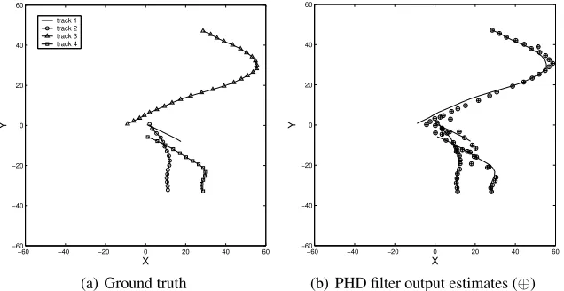
Fig. 1 Plots of 4 superimposed tracks over 40 time steps.
from the empirical probability distribution obtained by suitably normalis-ing it, to obtain a set ofLkparticles of equal weightnw(i)k /Nk, Xˆ k(i)oLk
i=1 – Rescale the weights to reflect the total mass of the system (i.e. multiply
the particle weights by a factor ofNkˆ ) giving the particle/weight ensemble
n
wk(i), Xk(i)oLk
i=1which definesα˜ Lk
k .
2.4 A Motivating Example
We present a brief example (which is taken from [14]) to illustrate the utility of the multi-object filtering framework and the SMC implementation of the PHD filter. Consider the problem of tracking an unknown number of targets that evolve in R4. For instance, in a two dimensional tracking example, each target could be described by itsxandycoordinates as well as its velocity in these directions. Existing targets can leave the surveillance area and new targets can enter the scene. At timek, a realisation of the state isXk = {xk,1, . . . , xk,M(k)} ⊂ R4. As for the observations, each target generates one observation with a certain probability (i.e. each target generates at most one observation) and, the sensors can measure false observations that are not associated with any target, i.e., clutter. Assume that sensors measure a noisy value of thexandycoordinate of a target. A realisation of the observation would beZk={zk,1, . . . , zk,N(k)} ⊂R2where measurement zk,icould either correspond to an element inXkor be a false measurement. Note that the number of observations need not coincide with the number of targets.
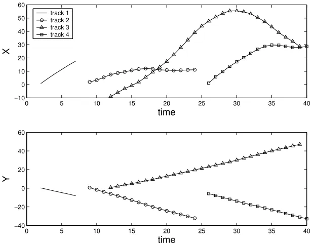
[image:9.612.77.395.43.207.2]timek, new targets can appear spontaneously according to a Poisson point process with an intensity functionγkset to0.2N(·; ¯x, Q), whereN(·; ¯x, Q)denotes a nor-mal density with meanx¯and uncertainty corresponding to the covariance,Q. This corresponds to one new target being created every five time steps around a location ¯
xwith covarianceQ. As for the observations, each target generates a noisy obser-vation of its position with certain probability. Additionally, false measurements are generated according to a Poisson point process with a uniform intensity function.
0 5 10 15 20 25 30 35 40 −10
0 10 20 30 40 50 60
X
time
0 5 10 15 20 25 30 35 40
−40 −20 0 20 40 60
Y
time
track 1 track 2 track 3 track 4
(a) Ground truth: plots ofxandycomponents of the 4 true tracks against time, showing
the different start and finish times of the tracks.
0 5 10 15 20 25 30 35 40
−100 −50 0 50 100
X
time
0 5 10 15 20 25 30 35 40
−100 −50 0 50 100
Y
time
(b)xandycomponents of position observations immersed in clutter of rater= 10.
[image:11.612.81.389.43.283.2]3 Convergence Study
It is shown that the integral of any bounded test function under the SMC approx-imation of the PHD filter converges to the integral of that function under the true PHD filter in mean of orderp(for all integerp) and hence almost surely. As ob-served by one referee, the restriction that test functions must be bounded seems more reasonable in the context of the PHD filter than the standard optimal filter as one is typically interested in the integrals of indicator functions. The result is shown to hold recursively by decomposing the evolution of the filter into a number of steps at each time. A number of additional points need to be considered in the present case. We assume throughout that the observation record{Zk}k≥0is fixed and generates the PHD recursion.
Remark 1As a preliminary, we need to show that both the true and approximate filters have finite mass at all times. In the case of the true filter this follows by as-suming that the mass is bounded at time zero and that||φk||∞is finite. Proceeding by induction we have:
˜
αk(1) =ΨkΦkαk˜ −1(1)
Φkαk˜ −1(1)≤γk(1) +||φk||∞αk˜ −1(1) ˜
αk(1)≤ |Zk|+γk(1) +||φk||∞αk˜ −1(1) (7) whilst, in the case of the particle approximation, it can always be shown to hold from the convergence towards the true filter at the previous time. Note that, when-ever we have a result of the form (10) or (11) together with (7) the total mass of the approximate filter must be finite with probability one and a finite upper bound upon the mass can be obtained immediately (consider theL1convergence result obtained by settingp= 1in (10) or (11)).
We make extensive use of [5, Lemma 7.3.3], the relevant portion of which is reproduced here.
Lemma 1 (Del Moral, 2004)Given a sequence of probability measures(µi)i≥1
on a given measurable space (E,E) and a collection of independent random variables, one distributed according to each of those measures,(Xi)i≥1, where ∀i, Xi ∼ µi, together with any sequence of measurable functions(hi)i≥1 such
thatµi(hi) = 0for alli≥1, we define for anyN ∈N,
mN(X)(h) = 1 N
N
X
i=1
hi(Xi) and σ2N(h) = 1 N
N
X
i=1
(sup(hi)−inf(hi))2
If thehi have finite oscillations (i.e.,sup(hi)−inf(hi) < ∞ ∀i ≥ 1) then we
have: √
NE[|mN(X)(h)|p]1/p≤d(p)1/pσN(h)
with, for any pair of integersn, psuch thatn≥p≥1, denoting(n)p=n!/(n− p)!:
d(2n) = (2n)n2−n and d(2n−1) =
(2n−1)n
q
n−1 2
We begin by showing that as the number of particles used to approximate the PHD filter tends towards infinity, the estimate of the integral of any bounded mea-surable function under the empirical measure associated with the particle approx-imation converges towards the integral under the true PHD filter in terms ofLp norm and that the two integrals areP−a.s. equal in the limit of infinitely many particles. The principal result of this section is theorem 1 which establishes the first result and leads directly to the second.
Throughout this section we assume that a particle approximation consisting of Lk−1weighted particles is available at timek−1, with associated empirical mea-sureα˜Lk−1
k−1 . These particles are propagated forwards according to the algorithm de-scribed previously, and an additionalJkparticles are introduced to account for the possibility of new objects appearing at timek. This gives us anMk=Jk+Lk−1 particle approximation, denotedαMk
k to the PHD filter at timek, which is subse-quently re-weighted (corresponding to the update step of the exact algorithm) and resampled to provide a sample ofLk particles at this time,α˜Lk
k . This leads to a recursive algorithm and provides a convenient decomposition of the error intro-duced at each time-step into quantities which can be straightforwardly bounded. We assume thatJk andMkare chosen in a manner independent of the evolution of the particle system, but which may be influenced by such factors as the number of observations.
3.1 Conditions
As a final precursor to the convergence study, we present a number of weak condi-tions which are sufficient for the convergence results below to hold. The following conditions are assumed to hold throughout:
– The particle filter is initialised with some finite mass byiidsampling from a tractable distributionα0˜ .
– The observation set is finite,|Zk|<∞∀k. – All of the importance ratios are bounded above:
sup (x,y)∈E×E
φkqk((x, yx, y))
< R1<∞ xsup∈E γkpk((xx))
< R2<∞ (8)
and that at least one of these ratios is also strictly positive.
– The individual object likelihood function is bounded above and strictly posi-tive:
– Resampling is done according to a multinomial scheme, that is the number of representatives of each particle which survives is sampled from a multinomial distribution with parameters proportional to the particle weights.
The first of these conditions simply constrain the initialisation of the parti-cle approximation, the next is a weak finiteness requirement placed upon the true system, the next two are implementation issues and are required to ensure that the importance weights and that the filter density remains finite. The penultimate condition prevents unstable interactions between the filter mass and the particle approximation.
3.2LpConvergence and Almost Sure Convergence
The following theorem is the main result of this section and is proved by induction. It is shown that each step of the algorithm introduces an error (in theLp sense) whose upper bound converges to zero as the number of particles tends to infinity and that the errors accumulated by the evolution of the algorithm have the same property.
Theorem 1 (LpConvergence)
Under the conditions specified in section 3.1, there exist finite constants such that for anyξ ∈ Bb(E),ξ:E→Rthe following holds for all timesk:
EhαMk
k (ξ)−αk(ξ)
pi
1/p
≤¯ck,p||√ξ||∞
Mk (10)
Ehα˜Lk
k (ξ)−αk˜ (ξ)
pi
1/p
≤ck,p||√ξ||∞
Lk (11)
Convergence in anLpsense directly implies convergence in probability, so we also
have:
αMk
k (ξ) p →αk(ξ) ˜
αLk
k (ξ) p →αk˜ (ξ)
Furthermore, by a Borel-Cantelli argument, the particle approximation of the in-tegral of any function with finite fourth moment converges almost surely to the integral under the true PHD filter as the number of particles tends towards infin-ity.
Proof.
Equation (11) holds at time 0 by lemma 2.
Now, if equation (11) holds at timek−1then, by lemmas 3 and 4, equation
(10) holds at timek.
Similarly, if equation (10) holds at timekthen by lemmas 5 and 6, equation
(11) also holds at timek.
Lemma 2 (Initialisation)If, at time zero, the particle approximation,α˜L00 , is ob-tained by takingL0iidsamples fromα0/˜ α0˜ (1)and weighting each byα0˜ (1)/L0, then there exists a finite constantc0,p such that, for allp ≥ 1and for all test functionsξinBb(E):
Ehα˜L00 (ξ)−α0˜ (ξ)
pi
1/p
≤c0,p||√ξ||∞ L0
Proof. This can be seen to be true directly by applying lemma 1. ut
Lemma 3 (Prediction)If, for some finite constantck−1,p, and all test functionsξ
inBb(E):
Ehα˜Lk−1
k−1 (ξ)−αk˜ −1(ξ)
pi1/p
≤ck−1,p || ξ||∞
p
Lk−1
Then there exists some finite constant ˆck,p such that, for all test functions ξ in Lp(E):
EhΦkα˜Lk−1
k−1 (ξ)−Φkαk˜ −1(ξ)
pi1/p
≤ck,pˆ p||ξ||∞
Lk−1
Proof. From the definition of the prediction operator:
EhΦkα˜Lk−1
k−1 (ξ)−Φkαk˜ −1(ξ)
pi
1/p
=Ehα˜Lk−1
k−1 φk(ξ)−αk˜ −1φk(ξ)
pi
1/p
=Ehα˜Lk−1
k−1 −αk˜ −1
φk(ξ)pi 1/p
Hence, by the assumption of the lemma:
EhΦkα˜Lk−1
k−1 (ξ)−Φkαk˜ −1(ξ)
pi1/p
≤ck−1,p
supζ|φk(ζ, ξ)|
p
Lk−1
≤ck−1,p
supζ,xφk(ζ, x)||ξ||∞
p
Lk−1
Which gives us the claim of the lemma with:ck,pˆ =ck−1,psupζ,xφk(x, ζ) ut Lemma 4 (Sampling)If, for some finite constant,ck,pˆ :
EhΦkα˜Lk−1
k−1 (ξ)−Φkαk˜ −1(ξ)
pi
1/p
≤ˆck,pp||ξ||∞
Lk−1
Then, there exists a finite constant˜ck,psuch that:
EhαMk
k (ξ)−αk(ξ)
pi
1/p
Proof. LetGk−1 be theσ−field generated by the set of all particles until time k−1. By a conditioning argument onGk−1, we may view
Yk(i)
i≥1as
indepen-dent samples with respective distributions qkYk(i),·
i≥1. Let α¨ Lk−1 k be the
empirical measure associated with the particlesYk(i)
i≥1after the re-weighting
step in equation (5), i.e.,
¨ αLk−1
k = LXk−1
i=1 ˜ w(i)k δY(i)
k
and define the sequence of functionshi(·) = φk(X (i)
k−1,·)ξ(·) qk(Xk(i−)1,·) −
φk(ξ)Xk(i)−1
and
associated measuresµi(·) =qk(Xk(i),·)such thatµi(hi) = 0. It is clear that:
¨ αLk−1
k (ξ)−α˜ Lk−1 k φk(ξ) ˜
αLk−1 k−1 (1)
= Lk−1
X
i=1
w(i)k−1hi(Y (i) k ) ˜
αLk−1 k−1 (1)
Which allows us to write:
Ehα¨Lk−1 k (ξ)−α˜
Lk−1 k φk(ξ)
pi =E α˜Lk−1
k−1 (1)
p E
Lk−1
X
i=1
w(i)k−1hi(Y (i) k ) ˜
αLk−1 k−1 (1)
p Gk−1
≤Ehα˜Lk−1 k−1 (1)
pi
2pd(p)
φk
qk
∞||ξ||∞ p
p
Lk−1 p
where the final inequality follows from an application of lemma 1. This gives us the bound:
Ehα¨Lk−1 k (ξ)−α˜
Lk−1 k φk(ξ)
pi1/p
≤ 2d(p) 1/pCα˜
k,pR1||ξ||∞ p
Lk−1
WhereCα
k,p is the finite constant which boundsEhα˜ Lk−1 k−1 (1)
pi 1/p (see remark 1).
If we allow˚αJk
k be the particle approximation toγk obtained by importance
sampling frompkthen it is straightforward to verify that, for some finite constant ˆ
Bkpobtained by using lemma 1 once again:
Eh˚αJk
k (ξ)−γk(ξ)
pi1/p
≤2d(p)1/p
γkpk ∞
||ξ||∞ √
And noting thatαMk
k = ˚α Jk
k + ¨α Lk−1
k we can apply Minkowski’s inequality to
obtain:
EhαMk
k (ξ)−Φkα˜ Lk
k−1
pi
1/p
≤2Ck,Pα d(p)1/p
φk qk
∞||ξ||∞ p
Lk−1
+2d(p)1/p
γkpk ∞
||ξ||∞ √
Jk
Defininglk−1 = Lk−1/Mk andjk = Jk/Mk for convenience, we arrive at
the result of the lemma with (making use of (8)):
˜
ck,p= 2d(p)1/pCk,pα R1
p
lk−1
+ 2d(p)1/p√R2jk
u t
Lemma 5 (Update)If for some finite constant˜ck,p:
EhαMk
k (ξ)−αk(ξ)
pi1/p
≤ck,p˜ ||√ξ||∞ Mk
Then there exists a finite constantck,p¯ such that:
EhΨkαMk
k (ξ)−αk˜ (ξ)
pi1/p
≤ck,p¯ ||√ξ||∞
Mk
Proof. The proof follows by expanding the norm and using Minkowski’s inequality to bound the overall norm. The individual constituents are bounded by the assump-tion of the lemma.
EhΨkαMk
k (ξ)−αk˜ (ξ)
pi
1/p
=E"
α
Mk
k νkξ+
X
z∈Zk
ψk,zξ κk(z) +αMk
k (ψk,z)
!
−αk νkξ+ X z∈Zk
ψk,zξ κk(z) +αk(ψk,z)
!
p#1/p
≤EhαMk
k (νkξ)−αk(νkξ)
pi 1/p + X
z∈Zk
E"αMk
k
ψk,zξ κk(z) +αMk
k (ψk,z)
!
−αk
ψk,zξ κk(z) +αk(ψk,z)
p#1/p
Noting thatνk is a probability, the first term is trivially bounded by the
as-sumption of the lemma:
EhαMk
k (νkξ)−αk(νkξ)
pi
1/p
≤˜ck,p||νk||√∞||ξ||∞ Mk ≤˜ck,p
||ξ||∞ √
In order to bound the second term a little more effort is required, consider a single element of the summation:
E"αMk
k
ψk,zξ κk(z) +αMk
k (ψk,z)
!
−αk
ψk,zξ κk(z) +αk(ψk,z)
p#1/p
≤E"αMk
k
ψk,zξ κk(z) +αMk
k (ψk,z)
!
−αMk
k
ψk,zξ κk(z) +αk(ψk,z)
p#1/p +
EαMk
k
ψk,zξ
κk(z) +αk(ψk,z)
−αk
ψk,zξ
κk(z) +αk(ψk,z)
p1/p
≤E
αMk
k (ψk,zξ)
h
κk(z) +αMk
k (ψk,z)
−(κk(z) +αk(ψk,z))i
κk(z) +αMk
k (ψk,z)
((κk(z) +αk(ψk,z)))
p 1/p +
EαMk
k
ψk,zξ κk(z) +αk(ψk,z)
−αk
ψk,zξ κk(z) +αk(ψk,z)
p1/p
≤2E
hαMk
k (ψk,z)−αk(ψk,z)
pi1/p ||ξ||∞ κk(z) +αk(ψk,z)
Where the final line follows from the positivity assumptions placed upon one of the weight ratios and the likelihood function. This allows us to assert that:
X
z∈Zk
E"αMk
k
ψk,zξ κk(z) +αMk
k (ψk,z)
!
−αk
ψk,zξ
κk(z) +αk(ψk,z)
p#1/p
≤2Zk||ξ||∞sup
z
EhαMk
k (ψk,z)−αk(ψk,z)
pi1/p κk(z) +αk(ψk,z)
≤ 2Zk˜ck,p√ ||ξ||∞
Mk supz
||ψk,z||∞ κk(z) +αk(ψk,z)
Combining this with the previous result and assumption (9) gives the result of the lemma with:
¯
ck,p= 1 + 2Zk˜ck,psup z
R3 κk(z) +αk(ψk,z) u
t
Lemma 6 (Resampling)If, for some finite constant,ck,p¯ :
EhΨkαMk
k (ξ)−αk˜ (ξ)
pi
1/p
≤ck,p¯ ||√ξ||∞ Mk
and the resampling scheme is multinomial, then there exists a finite constantck,p
such that:
Ehα˜Lk
k (ξ)−αk˜ (ξ)
pi
1/p
Proof.
By Minkowski’s inequality,
Ehα˜Lk
k (ξ)−αk˜ (ξ)
pi1/p
≤Ehα˜Lk
k (ξ)−Ψkα˜ Mk
k (ξ)
pi1/p
+EhΨkα˜Mk
k (ξ)−αk˜ (ξ)
pi1/p
By the assumption of the lemma:
EhΨkα˜Mk
k (ξ)−αk˜ (ξ)
pi1/p
≤¯ck,p||√ξ||∞ Mk
We can bound the remaining term by taking the expectation conditioned upon the sigma algebra generated by the particle ensemble prior to resampling, noting that the resampled particle set is iidaccording to the empirical distribution before resampling:
Ehα˜Lk
k (ξ)−Ψkα˜ Mk
k (ξ)
pi
1/p
≤Ck,pD Ck,pR || ξ||∞
√ Lk
whereCD
k,pis the upper bound onEhα˜ Mk
k
pi
1/p
approximation at the resampling stage (again, this must exist by remark 1) andCR
k,p is a constant given by Del
Moral’sLp-bound lemma, lemma 1.
Thus we have the result of the lemma with:
ck,p=Ck,pD Ck,pR + ¯ck,p
r
Mk Lk u
t
It would be convenient to establish time-uniform convergence results and the stability of the filter with respect to its initial conditions. However, the tools pio-neered by [5] and subsequently [10,3] are not appropriate in the present case: the PHD filter is not a Feynman-Kac flow and decoupling the “prediction” and “up-date” steps of the filter is not straightforward due to the inherent nonlinearity and the absence of a linear unnormalised flow. It is not obvious how to obtain such results under realistic assumptions.
4 Central Limit Theorem
4.1 Formulation
It is convenient to write the PHD slightly differently to equations (3) and (4) for the purposes of considering the central limit theorem. It is useful to describe the evolution of the PHD filter in terms of selection and mutation operations to allow the errors introduced at each time to be divided into the error propagated forward from earlier times and that introduced by sampling at the present time-step. The formulation used is similar to that employed in the analysis of Feynman-Kac flows [5] under an interacting-process interpretation.
We introduce a potential function, Gk,αk : E → R and its associated
se-lection operatorSk,αk : E ×E → Rand as the selection operator which we
employ updates the measure based upon the full distribution at the previous time, we may define the measureSk,αˆ
k(x) =αk(Sk,αk(·, x))αk(Gk,αk)/αk(1)which
is obtained by applying the selection operator to the measure and renormalising to correctly reflect the evolution of the mass of the filter:
Gk,αk(·) =νk(·) +
X
z∈Zk
ψk,z(·) κk(z) +αk(ψk,z)
Sk,αk(x, y) =
αk(y)Gk,αk(y)
αk(Gk,αk)
ˆ
Sk,αk(·) =αk(·)Gk,αk(·)
For clarity of exposition, we have assumed in this section thatN particles are propagated forward from each time step to the next and thatηkN particles are introduced to account for spontaneous births at timek(i.e., in the notation of the previous section,Lk =N andJk=ηkN). The notationNk= (1 +ηk)N is also used for notational convenience.
The interpretation of this formulation is slightly different and perhaps more intuitive. Update and resampling occur simultaneously and comprise the selection step, while prediction follows a mutation operation. Here we useαk to refer to the predicted filter as in (3), and it is not necessary to make any reference to the updated filter. We separate the spontaneous birth component of the measure from that which depends upon the past and write the PHD recursion as:
αk(ξ) = ˆαk(ξ) + ˚αk(ξ) ˆ
αk(ξ) = ˆSk−1,αk−1φk(ξ) ˚
αk(ξ) =γk(ξ)
4.1.1 The Particle Approximation Within this section, the particle approxima-tion described previously can be restated as the following iterative procedure. This provides an alternative view of the algorithm given in section 2.3.1, with the addi-tional assumption that the number of particles propagated forward at each time step is constant, and no explicit reference toαk˜Lk. As we are concerned with
1. Let the particle approximation prior to resampling at timek−1be of the form
αNk−1 k−1 =
1 N
Nk−1
X
i=1 ˜
wk(i)−1δX(i)
k−1
2. SampleNparticles to propagate forward via the selection operator:
Yk(i)←Sk
−1,αNk−1
k−1 (·)
N
i=1 3. Mutate theseNparticles.
n
Xk(i)←qk(Yk(i),·)oN i=1
4. IntroduceηkN particles to account for the possibility of births.
n
Xk(i)←pk(·)oNk i=N+1 5. Define the particle approximation at timekasαNk
k = ˆαNk + ˚α ηkN
k where: ˆ
αNk = 1 N
N
X
i=1 ˜ wk(i)δX(i)
k and˚α
ηkN
k = 1 N
Nk
X
i=N+1 ˜ w(i)k δX(i)
k
and the weights are given by:
˜ wk(i)=
αNk−1 k−1
G
k−1,αNk−1
k−1
φk(Yk(i),X
(i)
k )
qk(Yk(i),X
(i)
k )
i∈ {1, . . . , N}
1 ηk
γk(Xk(i))
pk(Xk(i))
i∈ {N+ 1, . . . , Nk}
4.2 Variance Recursion
Theorem 2 (Central Limit Theorem) The particle approximation to the PHD filter follows a central limit theorem with some finite variance for all continuous bounded test functionsξ:E→Rd, at all timesk≥0:
lim N→∞
√ NhαNk
k (ξ)−αk(ξ)
i d
→ N 0, σk2(ξ)
provided that the result holds at time0, which it does, for example, if the filter
is initialised by obtaining samples from a normalised version of the true filter by importance sampling and weighting them correctly.
Proof. By assumption, the result of the theorem holds at time0. Using induction the result can be shown to hold for all times by the sequence of lemmas, lemma 7-10, that follow.
The core of the proof is the following decomposition:
αNk
k (ξ)−αk(ξ) = ˆαNk (ξ)−Sˆk−1,αNk−1
k−1
qk×φkqk
(ξ) +
ˆ S
k−1,αNk−1
k−1
qk×φk qk
(ξ)−αkˆ (ξ) +
˚α(ηkN)
k (ξ)−˚αk(ξ)
Consistent with the notation defined in section 2.1,Sˆ
k−1,αNkk−−11
qk×φk
qk
(ξ)is to
be understood as Z
ˆ Sk
−1,αNk−1
k−1 (du)
Z
qk(u, dv)φk(u, v) qk(u, v)ξ(v)
i.e.,qk×φk
qk defines a new transition kernel fromEtoE.
The first term in this decomposition accounts for errors introduced at timek
by using a particle approximation of the prediction step and this is shown to con-verge to a centred normal distribution of varianceVkˆ (ξ)in lemma 7. The second
term describes the errors propagated forward from previous times, and is shown to follow a central limit theorem with varianceVk¨ (ξ)in lemma 8. The final term
corresponds to sampling errors in the spontaneous birth components of the filter and this is shown to follow a central limit theorem with variance˚Vk(ξ)in lemma
9.
Lemma 10 shows that the result of combining the three terms of the decom-position is a random variable which itself follows a central limit theorem with variance:
σ2
k(ξ) = ˆVk(ξ) + ¨Vk(ξ) + ˚Vk(ξ)
which is precisely the result of the theorem for scalar test functions.
In the case of vector test functions, the result follows by the Cramer-Wold de-vice, applied to any linear combination of their components, and the covariance matrix is denotedΣk(ξ) = [Σk(ξi, ξj)]. ut
Lemma 7 (Selection-prediction Sampling Errors)The selection-prediction sam-pling error (due to steps 2 and 3) at timekconverges to a normally distributed ran-dom variable of finite variance as the size of the particle ensemble tends towards infinity:
lim N→∞
√ N
ˆ
αNk(ξ)−Sˆk−1,αNk−1
k−1
qk×φk qk
(ξ)
d
Proof. Consider the term under consideration:
ˆ αN
k(ξ)−Sˆk−1,αNk−1
k−1
qk×φk qk
(ξ)
= 1 N N X i=1 ˜
wk(i)ξ(Xk(i))−Sˆ
k−1,αNkk−−11
qk×φk qk
(ξ)
= √1 N N X i=1 UN k,i x where
Uk,iN = ˜
wk(i)ξ(Xk(i))−Sˆ
k−1,αNkk−−11
qk×φk
qk
(ξ) √
N
LetHN k =σ
n
Xn(i),w˜n(i)
oNn
i=1:n= 0, . . . , k
be the sigma algebra generated by the particle ensembles occurring at or before timek and further letHN
k,j = σ
HN k−1,
n
Xk(i),w˜(i)k oj i=1
.
It is evident that conditioned upon HN k−1,
n
Yk(i), X (i) k
oN
i=1 are iidsamples
from the product distributionSk
−1,αNk−1
k−1
(y)qk(y, x)and, therefore:
EUk,iN
HN
k,i−1
=EUk,iN
HN
k−1
= 0
Furthermore, conditionally,UN
k,ihas finite variance, which follows from
assump-tion (8) and the assumpassump-tion that the observaassump-tion set and the initial mass of the filter are finite:
Eh UN k,i
2i
=EhEh UN k,i
2
HN k,i−1
ii
= 1
NE
"
˜
w(i)k ξ(Xk(i))2−
ˆ S
k−1,αNk−1
k−1
qk×φk qk
(ξ)
2#
<
2EαNk−1
k−1 (1) +|Zk−1|
2 R21||ξ||
2
∞
N <∞
Noting that, by the Lp convergence result of theorem 1 the expectation may be
bounded above uniformly in N. We have that∀t∈[0,1], >0:
lim N→∞
bXN tc
i=1
Eh Uk,iN
2
I|UN k,i|>
HN
k,i−1
i p
→0 (12)
converges to the product of their respective limits and that for nonzero random variables the same is true of the quotient of those sequences)
αNk−1 k−1
G k,αNk−1
k−1
αNk−1 k−1
G k,αNk−1
k−1
φk×φk qk
(ξ)
−αNk−1 k−1
G k,αNk−1
k−1 φk(ξ)
2
(13)
p
→αk−1 Gk,αk−1
αk−1
Gk,αk−1
φk×φkqk
(ξ)
−αk−1 Gk,αk−1φk(ξ)
2
(14)
it is apparent (as (13) is equal to N
bN tc times (15) and (14) to
1
t times (16)) that
bXN tc
k=1
Eh Uk,iN
2
HN k,i−1
i
=bN tc N α
Nk−1 k−1
Gk
−1,αNk−1
k−1
2 ×
Sk
−1,αNk−1
k−1
φk×φkqk
(ξ2)−Sk
−1,αNk−1
k−1
(φk(ξ))2
(15) p
→tαk−1 Gk−1,αk−1
2 ×
Sk−1,αk−1
φk×φk qk
(ξ2)−Sk−1,αk−1(φk(ξ)) 2
(16)
From this, it can be seen that for eachN, the sequence
Uk,iN,HNk,i
, 1≤i≤N
is a square-integrable martingale difference which satisfies the Lindeberg condi-tion (12) and hence a martingale central limit theorem may be invoked (see, for example, [13, page 543])) to show that:
lim N→∞ √ N ˆ
αNk (ξ)−Sˆk−1,αNk−1
k−1
qk×φkqk
(ξ)
d
→ N0,Vkˆ (ξ)
where,
ˆ
Vk(ξ) =αk−1 Gk−1,αk−1
2
Sk−1,αk−1
φk×φk qk
(ξ2)−Sk−1,αk−1(φk(ξ)) 2
=αk−1(Gk−1,αk−1) ˆSk−1,αk−1
φk×φkqk
(ξ2)−Skˆ−1,αk−1(φk(ξ)) 2
u t
Lemma 8 (Propagated Errors)The error resulting from propagating the particle approximation forward rather than the true filter has an asymptotically normal distribution with finite variance.
ˆ S
k−1,αNkk−−11
qk×φk qk
Proof. Direct expansion of the potential allows us to express this difference as:
ˆ Sk
−1,αNk−1
k−1
qk×φkqk
(ξ)−αkˆ (ξ)
= ˆS
k−1,αNkk−−11φk(ξ)−Skˆ−1,αk−1φk(ξ) =αNk−1
k−1
φk(ξ)G
k−1,αNkk−−11
−αk−1 φk(ξ)Gk−1,αk−1
=αNk−1
k−1 (φk(ξ)νk−1)−αk−1(φk(ξ)νk−1) +
X
z∈Zk−1 αNk−1
k−1 (∆k−1,z)−αk−1(∆k−1,z) κk−1(z) +α
Nk−1
k−1 (ψk−1,z)
where∆k−1,z =ψk−1,zφk(ξ)−κkα−k1(z)+α−1(ψk−k1−,z1(ψφkk(ξ))−1,z)ψk−1,zand the final equal-ity can be shown to hold by considering a single term in the summation thus:
αNk
k−1(ψk−1,zφk(ξ)) κk−1(z) +αNk−k1−1(ψk−1,z)
−κkαk−1(ψk−1,zφk(ξ))
−1(z) +αk−1(ψk−1,z)
= 1
κk−1(z) +αNk−k1−1(ψk−1,z)
h
αNk−1
k−1 (ψk−1,zφk(ξ))−αk−1(ψk−1,zφk(ξ))
+αk−1(ψk−1,zφk(ξ))−
κk−1(z) +αkN−k−11(ψk−1,z) κk−1(z) +αk−1(ψk−1,z)
αk−1(ψk−1,zφk(ξ))
#
= 1
κk−1(z) +αNk−k1−1(ψk−1,z)
h
αNk−1
k−1 (ψk−1,zφk(ξ))−αk−1(ψk−1,zφk(ξ))
+αk−1(ψk−1,z)−α Nk−1
k−1 (ψk−1,z) κk−1(z) +αk−1(ψk−1,z)
αk−1(ψk−1,zφk(ξ))
#
= α Nk−1 k−1
ψk−1,zφk(ξ)−κk−1(z)+ααk−1(ψk−k−1(ψ1,zkφ−k1(ξ))ψ,zφk(ξ))ψk−1,zk−1,z
κk−1(z) +αkN−k−11(ψk−1,z)
−αk−1
ψk−1,zφk(ξ)−κk αk−1(ψk−1,zφk(ξ))ψk−1,z
−1(z)+αk−1(ψk−1,zφk(ξ))ψk−1,z
κk−1(z) +αkN−k−11(ψk−1,z)
If we set
∆k−1=
h
νkφk(ξ), ∆k−1,Zk−1,1, . . . , ∆k−1,Zk−1,|Zk−1|
i
whereZi
k−1denotes theithelement of the setZk−1, and, ρNk−1
k−1 =
"
1, 1
κk−1(Zk−1,1) +α Nk−1
k−1 (ψk−1,Zk−1,1) , . . . ,
1 κk−1(Zk−1,|Zk−1|) +α
Nk−1
k−1 (ψk−1,Zk−1,|Zk−1|)
Then the quantity of interest may be written as an inner product: D
ρNk−1 k−1 , α
Nk−1
k−1 (∆k−1)−αk−1(∆k−1)
E
We know from theorem 1 thatρNk−1 k−1
p
→ρk−1, where
ρk−1=
1, 1
κk−1(Zk−1,1) +αk−1(ψk−1,Zk−1,1) , . . . ,
1
κk−1(Zk−1,|Zk−1|) +αk−1(ψk−1,Zk−1,|Zk−1|)
#T
And furthermore, we know by the induction assumption that eachαNk−1
k−1 (∆k−1)− αk−1(∆k−1)is asymptotically normal with zero mean and some known variance, Σk−1(∆k−1). By Slutzky’s theorem, therefore, the quantity of interest converges to
a normal distribution of mean zero and varianceVk¨(ξ) =ρT
k−1Σk−1(∆k−1)ρk−1. u
t
Lemma 9 (Spontaneous Births)The error in the particle approximation to the spontaneous birth element of the PHD converges to a normal distribution with finite variance:
lim N→∞
√
Nh˚αηkN
k (ξ)−˚αk(ξ)
i d
→ N0,Vk˚(ξ)
Proof.
˚αηkN
k (ξ)−˚αk(ξ) = γk(1)
ηkN Nk
X
j=N+1
γk(Xk(j)) γk(1)pk(Xk(j))ξ(X
(j) k )−
γk(ξ) γk(1)
!
Of course, the particles appearing within this sum areiidaccording topkand this corresponds toγk(1)multiplied by the importance sampling estimate giving us the standard result:
p
ηkN
"
˚ αηkN
k (ξ)−˚αk(ξ) γk(1)
#
d → N
0,Varpk
γk γk(1)pkξ
which is precisely the result of the lemma with:
˚
Vk(ξ) = 1 ηk
γk
γk
pkξ 2
−γk(ξ)2
u t
Lemma 10 (Combining Terms)Using the results of lemmas 7–9 it follows that
αNk
k (ξ)−αk(ξ)satisfies the central limit theorem: lim
N→∞
√ NαNk
k (ξ)−αk(ξ)
d
→ N(0, σk(ξ))
Proof. The proof follows the method of [10]. The characteristic function of the random variable of interest is
Υk(t) =Ehexpit√NαNk
k (ξ)−αk(ξ)
i
As the particles associated with the spontaneous birth term of the PHD are inde-pendent of those propagated forward from the previous time we can write:
Υk(t) =Ehexpit√N˚αηkN
k (ξ)−˚αk(ξ)
i
×Ehexpit√N αˆNk (ξ)−αkˆ (ξ)
i
The first term of this expansion is the characteristic function of a normal random variable, so all that remains is to show that the same is true of the second term. Using the same decomposition as above, we may write:
Ehexpit√N αˆkN(ξ)−αkˆ (ξ)
i =E A
z }| {
E
exp
it√N
ˆ
αNk(ξ)−Sˆk−1,αNk−1
k−1
qk×φkqk
(ξ)HN k−1
×exp
it√N
ˆ S
k−1,αNkk−−11
qk×φk qk
(ξ)−αkˆ (ξ)
| {z }
B =E "
A−exp −t 2Vkˆ (ξ)
2
!! B
#
+ exp −t 2Vkˆ (ξ)
2
! E[B]
All that remains is to show that the first term in this expansion vanishes and we will have shown that the characteristic function of interestΥk(t)corresponds to
a Gaussian distribution as it can be expressed as the product of three Gaussian characteristic functions. Furthermore, it must have variance equal to the sum of the variances of the three constituent Gaussians which is exactly the result which we wish to prove.
By the conditionallyiidnature of the particles, we can write:
A=E
exp it N X j=1 Uk,jN
H N k−1
=Eexp itUk,1NHNk−1
N Hence:
A−exp −
t2Vkˆ (ξ) 2 ! = E
exp itUN
k,1HkN−1
N
−exp −t
Using the same result as [10] (i.e. that|uN −vN
| ≤N|u−v|∀|u| ≤1,|v| ≤1) we obtain:
A−exp −
t2Vkˆ (ξ) 2 ! ≤N E
exp itUk,1NHNk−1
−exp −t
2Vkˆ(ξ)/N 2
!
The following decomposition can be used to show that this difference converges to zero asN→ ∞:
E "
exp itUN k,1
−exp −t
2Vkˆ (ξ)/N 2
!
H
N k−1
#
=Eexp itUk,1NHkN−1
− 1−t 2(UN
k,1)2 2
!
+ (17)
1−t 2(UN
k,1)2 2 ! −exp −t 2 2E h
Uk,1N
2
HkN−1
i + (18) exp −t 2 2E h
Uk,1N
2
HNk−1
i
−exp −t
2Vkˆ(ξ)/N 2
!
(19)
We now show that the product ofN and the expectation of each of these terms converges to zero. First, consider (17). We can representeiy as1 +iy
− y22 +
|y|3
3! θ(y)for some suitable functionθ(y),|θ| < 1. Thus, as U N
k,1 is a martingale
increment: E "
exp itUk,1N
− 1−t 2(UN
k,1)2 2
!
H
N k−1
# ≤ t 3 6E h Uk,1N
3HN
k−1
i
≤ t
3 6N3/22
3
||ξ||3∞αNk−1
k−1 (1)R1+|Zn−1|R1
3
AndNtimes the expectation of this quantity converges to zero asN → ∞. To deal with (18) note that1−u≤exp(−u)≤1−u+u2 ∀u≥0. Setting
u=t 2 2E
h
Uk,1N
2
HNk−1
i
one obtains:
E" 1−t 2(UN
k,1)2 2 ! −exp −t 2 2E h
Uk,1N
2
HN k−1
i H N k−1
#
≤ t 4 4E
h
Uk,1N
2
HN k−1
i2
≤ t 4 4
1 N24||ξ||
4
∞
αNk−1
k−1 (1)R1+|Zk−1|R1
and once again, the expectation ofN times the quantity of interest converges to zero.
Finally, (19) can be shown to vanish by considering the following exponential bound. Forv≥u≥0, we can write|e−u
−e−v
| ≤ |1−eu−v
| ≤ |u−v|where the final inequality corresponds to [1, 4.2.32] and this gives us:
exp
−t 2 2E
h
Uk,1N
2
HN k−1
i
−exp −t
2Vkˆ (ξ)/N 2
!
≤ t 2 2N
NE
h
Uk,1N
2
HN k−1
i2
−Vkˆ(ξ)
which can be exploited by noting that:
NEh Uk,iN
2
HN k,i−1
i
=
αNk−1
k−1 (Gk−1,αNk−1
k−1 ) ˆSk
−1,αNk−1
k−1
φk×φkqk
(ξ2)
−Sˆk
−1,αNk−1
k−1
(φk(ξ))2
(20)
ˆ Vk(ξ) =
αk−1(Gk−1,αk−1) ˆSk−1,αk−1
φk×φk qk
(ξ2)
−Skˆ−1,αk−1(φk(ξ))
2i (21)
As (20) converges to (21) in probability (cf lemma 8) and (20) is bounded above, (20) converges to (21) inL1and the result we seek follows. Consequently,
(19) vanishes and we have the result of the lemma. ut
References
1. M. Abramowitz and I. A. Stegun, editors. Handbook of Mathematical Functions. Dover, ninth printing edition, 1970.
2. P. Billingsley.Probability and Measure. Wiley Series in Probability and Mathematical Statistics. John Wiley and Sons, second edition, 1986.
3. N. Chopin. Central limit theorem for sequential Monte Carlo methods and its applica-tions to Bayesian inference.Annals of Statistics, 32(6):2385–2411, December 2004. 4. D. J. Daley and D. Vere-Jones.An Introduction to the Theory of Point Processes,
vol-ume I: Elementary Theory and Methods ofProbability and Its Applications. Springer, New York, second edition, 2003.
5. P. Del Moral. Feynman-Kac formulae: genealogical and interacting particle systems with applications. Probability and Its Applications. Springer Verlag, New York, 2004. 6. P. Del Moral and A. Guionnet. Central limit theorem for non linear filtering and
inter-acting particle systems.Annals of Applied Probability, 9(2):275–297, 1999.
7. A. Doucet, N. de Freitas, and N. Gordon, editors. Sequential Monte Carlo Methods in Practice. Statistics for Engineering and Information Science. Springer Verlag, New York, 2001.
9. I. R. Goodman, R. P. S. Mahler, and H. T. Nguyen. Mathematics of Data Fusion. Kluwer Academic Publishers, 1997.
10. H. R. K¨unsch. Recursive Monte Carlo filters: Algorithms and theoretical analysis. Re-search Report 112, ETH: Seminar F¨ur Statistik, 2003. To appear inAnnals of Statistics. 11. R. P. S. Mahler. Multitarget Bayes filtering via first-order multitarget moments.IEEE
Transactions on Aerospace and Electronic Systems, 39(4):1152, October 2003. 12. C. P. Robert and G. Casella. Monte Carlo Statistical Methods. Springer Verlag, New
York, second edition, 2004.
13. A. N. Shiryaev. Probability. Number 95 in Graduate Texts in Mathematics. Springer Verlag, New York, second edition, 1995.