University of Warwick institutional repository: http://go.warwick.ac.uk/wrap
This paper is made available online in accordance with
publisher policies. Please scroll down to view the document
itself. Please refer to the repository record for this item and our
policy information available from the repository home page for
further information.
To see the final version of this paper please visit the publisher’s website
.
Access to the published version may require a subscription.
Author(s): B Cassella and GO Roberts
Article Title: Exact Monte Carlo Simulation of Killed Diffusions
Year of publication: 2007
Link to published article:
http://www2.warwick.ac.uk/fac/sci/statistics/crism/research/2007/paper
07-26
Exact Monte Carlo Simulation of Killed
Diffusions
Bruno Casella; Gareth O. Roberts
November 15, 2007
Abstract
We describe and implement a novel methodology for Monte Carlo sim-ulation of one-dimensional killed diffusions. The proposed estimators represent an unbiased and efficient alternative to current Monte Carlo estimators based on discretization methods for the cases when the finite-dimensional distributions of the process are unknown. For barrier option pricing in finance, we design a suitable Monte Carlo algorithm both for the single barrier case and the double barrier case. Results from numerical investigations are in excellent agreement with the theoretical predictions.
1
Introduction
Many important problems can be reduced to the computation of the expected value, sayν, of a functional of a diffusion processX. In this paper, we will derive and implement efficient and unbiased methods for Monte Carlo evaluation ofν when analytical expressions for the finite -dimensional distributions of X are not available and the value of the functional depends on barriers (either a single barrier or double barriers).
We consider a one-dimensional diffusion processX:
dXt=μ(Xt)dt+σ(Xt)dWt; X0=x0, (1) 0≤t≤T
where{Wt: 0≤t≤T}is a standard Brownian Motion and the driftμand the diffusion coefficientσare presumed to satisfy the usual conditions that guarantee the existence of a weakly unique global solution of (1) (see e.g. Chapter 5 of Oksendal, 1998).
Let H := (a, b) be an open interval of R such that X0 = x0 ∈ H. We are interested in the computation of:
where T >0 is a fixed time, τ is the first exit time of X from the set H and h(·) is a measurable function.
In mathematical finance, the problem of the computation of (2) arises in many contexts, e.g. in barrier options pricing (e.g. Merton, 1973; Reiner and Ru-binstein, 1991) or in structural credit risk modeling (e.g. Black and Cox, 1976; Longstaff and Schwarz, 1995). Analytic computation of (2) is only possible for a limited collection of simple models. For example, in the Black-Scholes case, Reiner and Rubinstein (1991) derived an explicit formula for the price of sin-gle barrier options of European style. Recently Davydov and Linetsky (2001) extended these results to asset processes driven by CEV diffusions. However in general we have to approximate (2) by Monte Carlo methods.
1.1
Background
In principle, when using Monte Carlo simulation, many trajectories ofX are generated and the value of the functional is evaluated at each sample path. Av-eraging over all paths provides then an unbiased estimator ofν which converges to the true value as the number of iterations increases. When the transition den-sities ofX are not known, common practice introduces some kind of discrete approximation ˜X of the processX. From the discrete approximation, suitable estimates for expected functions can be derived. The simplest and most popular of these methods is the Euler discretization which approximates (1) by means of:
˜
XiΔ= ˜X(i−1)Δ+μ( ˜X(i−1)Δ)Δ +σ( ˜X(i−1)Δ)
√
Δi; X˜0=x0, (3) (i= 1,2, . . . , n)
˜
Xt= ˜X(i−1)Δ+μ( ˜X(i−1)Δ)(t−(i−1)Δ) +σ( ˜X(i−1)Δ)(Wt−W(i−1)Δ) (4)
The idea here is to produce a realisation of the process (3) generating ˜
XΔ,X˜2Δ, . . . ,X˜nΔ. Then for any two points ˜X(i−1)Δ and ˜XiΔ, we sample a [0,1]-uniformly distributed random variable and compare it with the crossing probability of the corresponding Brownian bridge. Schemes based on Brownian bridge interpolation of the Euler trajectories can be succesfully applied to many simulation probelms. Asmussen and Glynn (2007) apply analogous ideas to the exact simulation of reflected Brownian motion with drift and to the approxi-mation of reflected diffusions. These methods improve the rate of convergence of the discrete Euler scheme; in particular Gobet shows that the weak error is now of order n−1. However, when n is large, the use of (4) for Monte Carlo simulation ofν can be computationally expensive involving the simulation of a very large number of uniform random variables at each iteration of the Monte Carlo algorithm.
1.2
A new approach
We will describe and implement a new method for Monte Carlo estimation ofν. Our method is designed to deal with those cases when the family of transition densities of the processX is not available. In fact it improves the performances of Monte Carlo algorithms based on discretization methods in two directions.
• The Monte Carlo estimator is simulated exactly, so no bias is introduced in the simulation. Because of this, we call our method theExact Monte
Carlo method.
• There is no trade-off between accuracy of the estimation and computa-tional effort. The higher the level of approximation required, the larger the computational efficiency advantage gained by use of the exact algo-rithm.
We shall see that the exact algorithm approach is actually highly computation-ally efficient, often requiring less computing effort than rather crude discretiza-tion methods.
of interest. In Section 2, after some preliminaries, we state the mathematical results that justify the Monte Carlo procedure. In Section 3 we describe in details the Exact Monte Carlo algorithm. In Section 4 we introduce some further probabilistic constructions supporting more general versions of our algorithm. In Section 5 we report the results of a numerical study comparing the performance of our Monte Carlo estimator with the Monte Carlo estimators generated by (3) and (4). We end in Section 6 with some comments and concluding remarks.
2
Theoretical framework
2.1
The model
In this subsection, we describe the classDof one-dimensional diffusion processes (1) for which the Exact Monte Carlo method can be applied. We introduce the transformed processY :={Yt; 0≤t≤T}defined by
Yt=η(Xt) =
Xt
z 1
σ(u)du (5)
wherezcan be any element of the state space ofX. Assuming thatσis nowhere 0 and continuously differentiable, by Ito’s formula, the processY satisfies the SDE:
dYt=α(Yt)dt+dWt; Y0=η(x0) =y0 (6)
whereα(u) = μ(η −1(u))
σ(η−1(u))−12σ
η−1(u)andη−1denotes the inverse transforma-tion. LetC=C([0, T],R) be the set of the continuous functions from [0, T] to R,C theσ−algebra generated by the cylinder subsets ofC and{Ct:t∈[0, T]} the corresponding filtration. We denote by ω = {ωs: 0≤s≤T} the generic element ofC. LetQdenote the probability measure induced by the processY in (6) on (C,C) and W the corresponding measure induced by the Brownian motion with starting pointy0. We introduce the following conditions onY:
B0 Q<<Wand Girsanov representation holds:
dQ
dW(ω) = exp
T
0 α(ωt)dωt− 1 2
T
0 α 2(ω
t)dt
(7)
B1 The drift functionαisC1 (differentiable with continuity)
B2 The function (α2+α)/2 is bounded
ConditionsB0−B2 define the classDof diffusions (1) of interest:
2.2
Preliminaries
Roughly speaking, the Exact Algorithm 1 (EA1) (Beskos et al., 2006a) exploits a transformation of the likelihood ratio (7) to allow a rejection sampling on the path spaceCin order to simulate from the (unknown) diffusion measureQ. B1 andB2 permit the Girsanov ratio to be bounded by an explicit and everywhere finite function ofωT, which in turn permits an appropriate rejection sampling algorithm to be constructed. This construction is described in details Beskos and Roberts (2005), Beskos et al. (2006a) and Beskos et al. (2006b). Explicit links betweenB1 andB2 and the Conditions 1-3 in Beskos and Roberts (2005) (pp. 2425-2426) are provided in Appendix 2. EA1 returns as output a partial exact representation of the diffusion path, i.e. a collection of points of the trajectory ofY, including the (given) starting point at time 0 and the ending point at timeT. We call itSkeleton of the process and we represent it as:
S1:={(t0, y0),(t1, y1), . . . ,(tm, ym)} (8)
where 0 =t0 < t1 <· · ·< tm=T. Before stating the relevant results on EA1 we fix some preliminary notation. LetW(s,x;t,y) be the probability measure of a Brownian bridge starting at time s at locationx and finishing at time t at locationy. We also introduce the following representation of the exit times: for any measurable setB ⊂R
τB:= inf{t∈[0, T] :ωt∈/B}
under the convention inf{∅}= +∞. We will denote byqW(s, x;t, y;l1, l2) the exit probability of the (s, x)→(t, y) Brownian bridge from a given set (l1, l2) under the conditionx, y ∈(l1, l2):
qW(s, x;t, y;l1, l2) :=W(s,x;t,y)τ(l1,l2)≤T|x, y∈(l1, l2)
(9)
2.3
EA1 results
The following theorem brings together the relevant results from Beskos et al. (2006a). It states the conditions on (6) that allow the application of EA1 and it characterises the conditional law of the processY given the Skeleton.
Theorem 1
Under conditionsB0−B2 we can apply EA1 to simulate a Skeleton (8) of the processY. For any eventB∈ C:
Q(B) =ES1
WS1(B) (10)
whereWS1 := m
Therefore the conditional law of the processY given the Skeleton is the product law of Brownian bridges connecting the points of the Skeleton. This implies that, by conditioning onS1, we reduce the problem of the simulation from an unknown probability measureQto the problem of the simulation from Brownian bridge measures. The following result provides a simple application of this construction.
Corollary 1
LetS1 be the Skeleton ofY generated by EA1. Then, for anyl1< y0< l2:
Qτ(l1,l2)> T
=ES1
m
i=1
1−qW(ti−1, yi−1;ti, yi;l1, l2)
I{yi∈(l1,l2)}
(11)
Proof:
For anyi= 1,2, . . . , m, letCibe the set of continuous functions on [ti−1, ti] and
Ci the correspondingσ−algebra. We define the following events:
Bi:={ωt∈(l1, l2); ti−1≤t≤ti} ∈ Ci
Thenτ(l1,l2)> T
=B1×B2× · · · ×Bm so that from (10) and the definition ofWS1:
Qτ(l1,l2)> T
= ES1
m
i=1
W(ti−1,yi−1;ti,yi)(B
i)
= ES1
m
i=1
1−qW(ti−1, yi−1;ti, yi;l1, l2)
I{yi∈(l1,l2)}
2.4
Crossing probability of the Brownian bridge
2.4.1 One-sided crossing probability
We recall the problem of the evaluation of the crossing probability (9) for Brow-nian motion. Let us assumel1=−∞. It turns out that for anyl2∈R:
qW(s, x;t, y;−∞, l2) = exp
−2(l2−y)(l2−x) t−s
(12)
2.4.2 Two-sided crossing probability
The problem of determining the two-sided crossing probability of the Brownian bridge is more challenging than the one-sided problem. Although it has been ex-tensively studied in literature (see e.g. Bertoin and Pitman, 1994), a closed form expression is not available. In fact available representations are given in terms of an infinite sum. Nevertheless here we state a convergence result (Proposition 1) which will allow us to construct a suitable Monte Carlo algorithm for the double barrier case. Our approach relies on classical results of Doob (1949) and Anderson (1960). For a recent reference, see also P¨otzelberger and Wang (2001). In the Appendix, while proving Proposition 1, we will give a brief account of these constructions. Before stating the proposition we need some additional notation. For anyj∈Nwe introduce the two functions:
Pj(s, x;t, y;l1, l2) :=pj(s, x;t, y;l2−l1, l1) +pj(s, x;t, y;l2−l1, l2) Qj(s, x;t, y;l1, l2) :=qj(s, x;t, y;l2−l1, l1) +qj(s, x;t, y;l2−l1, l2)
where
pj(s, x;t, y;δ, l) = e−
2
t−s[jδ+(l−x1)][jδ+(l−y)]
qj(s, x;t, y;δ, l) = e−
2j
t−s[jδ2−δ(l−x)]
Furthermore we need the two sequences of real numbers:
nk(s, x;t, y;l1, l2) = k
j=1
[Pj(s, x;t, y;l1, l2)−Qj(s, x;t, y;l1, l2)] (13)
nk(s, x;t, y;l1, l2) = nk−1(s, x;t, y;l1, l2) +Pk(s, x;t, y;l1, l2) (14)
Proposition 1
For any−∞< l1< l2<+∞, ask→ ∞
nk(s, x;t, y;l1, l2) ↑ qW(s, x;t, y;l1, l2) (15) nk(s, x;t, y;l1, l2) ↓ qW(s, x;t, y;l1, l2) (16)
Proof:
In the Appendix.
3
The Exact Monte Carlo algorithm
3.1
General setting
After setting up the theoretical framework, we turn to the description of the Monte Carlo algorithm. In the first place we notice that since the functionη (5) is monotone increasing we can express expectation (2) under the measureQ of the transformed processY as
ν=EQh(ωT)I{τH>T} (17)
with h(·) = hη−1(·), H := (a, b), a = η(a) and b = η(b). Assuming X ∈ D, Theorem 1 ensures that we can apply EA1 to simulate a SkeletonS1 (8) ofY. Our simulation strategy will then consist of three main steps:
Step 1: we simulate a SkeletonS1 ofY (EA1)
Step 2: givenS1, we simulate an unbiased estimator ofν in (2)
Step 3: we simulate the Monte Carlo estimator by repeating and averaging.
Under the measureQ, we can define the two unbiased estimators ofν,
Plain vanilla: φ:=φ(ω) =h(ωT)I{τH>T} (18)
Rao-Blackwellised: ψ:=ψ(S1) =EQ[φ| S1] (19)
generating the Monte Carlo estimators:
˜ ν =
N j=1φ(j)
N ; νˆ=
N j=1ψ(j)
N
whereφ(j)j=1,2,...,N and ψ(j)j=1,2,...,N are sequences of i.i.d copies of (18) and (19). We will focus on the problem of the simulation of ˜ν and ˆν (step 2) given the Skeleton. Instead for the simulation of the Skeleton and the issues related to the implementation of EA1 (step 2) we refer to Beskos et al. (2006a).
3.2
Plain vanilla Monte Carlo estimator
QI{τH>T}= 1| S1
= Q(τH > T | S1) (20)
= m
i=1
1−qW(ti−1, yi−1;ti, yi;a, b)
I{yi∈H}
where the second equality follows from Corollary 1. Simulation from (20) in-volves the generation of independent events, say {Ei}i=1,2,...,m, of probabili-tiesqW(ti−1, yi−1;ti, yi;a, b)
i=1,2,...,m. These events are in fact the crossing events of the Brownian bridges selected byS1. If any Ei occurs we setφ≡0, otherwiseφ≡h(ym). The basic structure of the algorithm is outlined in Algo-rithm 1.
Algorithm 1Plain vanilla Monte Carlo algorithm
1. Call EA1 and simulate the SkeletonS1={(t0, y0),(t1, y1), . . . ,(tm, ym)}.
2. EvaluateI(S1) =1mI{yi∈H}.
IfI(S1) = 0 go to 5.
Otherwise go to 3.
3.1. Seti= 1.
3.2. Simulate the eventEi w.p. qW(ti−1, yi−1;ti, yi;a, b).
IfI{Ei}= 1 goto5.
Else ifi=m goto4. 3.3. Seti=i+ 1 and goto3.2.
4. Outputφ=h(ym).
5. Outputφ= 0.
6. Repeat 1-5 a sufficiently large number N of times and output
ˆ
ν = (1/N)Nj=1φ(j).
ni,k := nk(ti−1, yi−1;ti, yi;a, b)
ni,k := nk(ti−1, yi−1;ti, yi;a, b) (i= 1,2, . . . , m; k∈N)
Algorithm 2Subroutine to simulate the indicator variableI{Ei} (2 barriers)
3.2.1. SampleU ∼Unif[0,1]. Setk= 1.
3.2.2. Evaluateni,k andni,k.
IfU > ni,k go to3.2.3.
IfU < ni,k go to3.2.4.
Else setk=k+ 1repeat3.2.2.
3.2.3. Setk=Ni andoutputI{Ei}= 0.
3.2.4. Setk=Ni andoutputI{Ei}= 1.
Clearly, for any i = 1,2, . . . , m, the efficiency of the sampling scheme in Al-gorithm 2 is strictly connected to the behaviour of the random variable Ni representing the number of times we need to repeat the control until a decision is taken. The following proposition guarantees that, for anyi= 1,2, . . . , m,Ni has finite moments of every order.
Proposition 2
Let Mi(α) be the moment generating function of Ni. Then, for any i = 1,2, . . . , m, there existsi∈Rsuch that for any α∈(−i,+i):
Mi(α)<∞
Proof:
We prove the proposition for an arbitraryi∈ {1,2, . . . , m}. For the construction of the algorithm, for anyk= 1,2, . . .:
P r(Ni > k) =P r(U ∈(ni,k,min{1, ni,k})≤ni,k−ni,k
Mi(α) = E(eαNi) =
∞
k=0
e(k+1)α(P r(Ni> k)−P r(Ni> k+ 1))
≤ ∞
k=0
e(k+1)αP r(Ni> k) =eα
∞
k=0
ekαP r(Ni> k)
= eα+eα
∞
k=1
ekαP r(Ni > k)≤eα+eα
∞
k=1
ekα(ni,k−ni,k)
Mi(α) is finite for those values ofαfor which it converges the infinite series:
∞
k=1
ekα(ni,k−ni,k) =
∞
k=1
e−Δ2ki[kδi2+δi(b−x2)−δi(b−x1)−Δ2iα]
+
∞
k=1
e−Δ2ki[kδ 2
i−δi(a−Si)+δ(a−Si−1)−Δ2iα]
where Δi =ti−ti−1. It is now clear that it exists a neighborhood (−i,+i) of 0 such that, ifα∈(−i,+i) the two series on the right hand side converge; that isMi(α) is finite in (−i,+i).
It is worth remarking that in practice the algorithm performs surprisingly well. In fact, for anyi= 1,2, . . . , m,Niis typically very small since the two sequences
{nk}k=1,2,... and{nk}k=1,2,... converge to qW faster than exponentially. In the numerical example we will present in Section 5 we have verified that in the most of cases the algorithm comes to a decision after one or two iterations.
3.3
Rao-Blackwellised Monte Carlo estimator
Expanding the conditional expectation in (19) we obtain:
ψ=h(ym) m
i=1
1−qW(ti−1, yi−1;ti, yi;a, b)
I{yi∈H} (21)
Expression (21) shows that the simulation ofψrequires the analytical evaluation of the crossing probabilities of Brownian bridges. As we are aware, this is possible only in the single barrier case. So, assuming for example an upper barrier (a=−∞), from (12), we obtain:
ψ=ψ(S1) =h(ym)
m
i=1
1−exp
−2(b
−y
i)(b−yi−1) ti−ti−1
I{yi∈(−∞,b)}
In this context the simulation ofψ requires only the simulation ofS1 and the evaluation of expression (22). Repeating the procedure and averaging give an estimate of ˆν. The final Algorithm 3 turns out to be very simple. Unfortunately, in the double barrier case, Rao-Blackwellisation is not feasible since we are not able to evaluate analytically crossing probabilities in (21).
Algorithm 3Rao-Blackwellised Monte Carlo Algorithm (upper barrier)
1. Call EA1 and simulate the SkeletonS1.
2. Evaluateψ=ψ(S1)according to (22).
3. Repeat 1-2 a sufficiently large number N of times and output
ˆ
ν= (1/N)Nj=1ψ(j)
We point out that, if available, the Rao-Blackwellised estimator is preferable to the plain vanilla. In fact, by Jensen inequality:
Var (ψ)≤Var (φ) (23)
which implies that under a quadratic loss function, for fixed N, ˆν is more ef-ficient than ˜ν. Furthermore, the simulation of ˆν is computationally less de-manding than the simulation of ˜ν. In fact at each iteration of the Monte Carlo algorithm the simulation ofψinvolves only the simulation of the Skeleton, while the simulation ofφinvolves the simulation of the Skeleton and the simulation ofφfromQ|S1.
4
More general constructions
4.1
Exact Monte Carlo via a truncation of the drift
We consider now the problem of the Monte Carlo estimation ofν (17) given a family of diffusion processes (6) satisfyingB0 and the following two conditions:
B1∗ The drift functionαis differentiable on the closure H ofH
B2∗ The function (α2+α)/2 is bounded onH
Under the conditions above, by truncating the drift functionαat the barriers a andb and using smoothing techniques, it is possible to define a process ˜Y:
that satisfies the desirable conditionsC0−C2 (Section 2.1) and such that, for anyu∈H, ˜α(u)≡α(u). We denote by ˜Qthe measure induced by the process
˜
Y on the measurable space (C,C).
Theorem 2
Let us consider the two processesY andY˜ with SDEs (6) and (24). Ifα≡α˜for eachu∈H and the functionφ:C→Ris measurable with respect to CT∧τH
then:
EQ[φ(ω)] =EQ˜[φ(ω)]
Proof:
By Girsanov Theorem, the Radon-Nikodym derivative ofQwith respect to ˜Q is given by
MT(ω) = d
Q
dQ˜(ω) =
eR0Tα(ωs)dωs−12
RT
0 α2(ωs)ds
eR0Tα(ω˜ s)dωs−12
RT
0 α˜2(ωs)ds
By the measurability assumption onφand the martingale property of{Mt,Ct}0≤t≤T we have:
EQ[φ(ω)] = EQ˜[φ(ω)MT(ω)] =EQ˜
EQ˜φ(ω)MT(ω)| CT∧τH
= EQ˜
φ(ω)EQ˜MT(ω)| CT∧τH
=EQ˜φ(ω)MT∧τH
Since on the interval [0, T ∧τH) the two drift functions α and ˜α coincide, it turns out thatMT∧τH = 1, ˜Q-almost surely . The conclusion then follows.
In our framework, since φ(ω) =h(ωT)I{τH>T} is clearly CT∧τH-measurable,
Theorem 2 implies that
ν=EQh(ωT)I{τH>T}
=EQ˜h(ωT)I{τH>T}
(25)
4.2
Exact Monte Carlo via the Exact Algorithm 2
We replace conditionB2 with the following less restrictive condition:
B2∗∗ For all u ∈ R, (α2+α)/2 is bounded below and it is bounded above
either on (−∞, u)or on (u,+∞)
We assume without loss of generality that the function (α2+α)/2 is bounded on the intervals{(u,+∞)}u∈R. EA2 was introduced by Beskos et al. (2006a). A crucial difference between it and EA1 lies in the fact that it outputs a richer structure thanS1 (8). In fact in addition to the starting point (0, y0) and the ending point (T, yT) of the diffusion path, it includes also its minimum and the time at which this minimum is achieved, say (t∗, y∗). It is convenient to choose a representation ofS2 which takes into account this underlying structure:
S2:={(t0, y0),(t1, y1), . . . ,(tm1, ym1), . . . ,(tm2, ym2)} (26)
where 0 =t0< t1<· · ·< tm1 =t∗<· · ·< tm2 =T so that the minimum can
be easily identified as (tm1, ym1)≡(t∗, y∗). We denote byQ−y∗the probability
measure induced by the processY −y∗:={Yt−y∗: 0≤t≤T}on (C,C) and
W(s,x;t,y)+ the probability measure of a 3-dimensional Bessel bridge from (s, x) to (t, y). Furthermore we will denote crossing probabilities as follows:
qW+(s, x;t, y;l
1, l2) :=W(s,x;t,y)+
τ(l1,l2)≤T |x, y∈(l1, l2)
The following result is the analogous of Theorem 1 and it can be derived from the construction presented in Beskos et al. (2006a)
Theorem 3
Under conditionsC0, C1 and B2∗∗ we can apply EA2 to simulate a Skeleton
S2(26) of the processY. For any eventA∈ C:
Q−y∗(A) =ES2
WS2
+(A)
whereWS2+ = m2
i=1W(ti−1,yi−1−y ∗;t
i,yi−y∗)
+ .
Theorem 3 justifies the following suitable representation of the crossing proba-bility of the processY.
Corollary 2
LetS2 be the Skeleton ofY generated by EA2. Then, for anyl1< y0< l2:
Qτ(l1,l2)> T
=ES2
I{y∗>l1} m2
i=1
1−qW+t
i−1, yi∗−1;ti, yi∗;−∞, l∗2
I{Ci}
(27)
Proof:
From Theorem 3 we derive the following representation:
Qτ(l1,l2)> T
=Q−y∗τ(l∗
1,l∗2)> T
=ES2
WS2+ τ(l∗
1,l∗2)> T
where we have setl1∗ =l1−y∗. Proceeding as in the proof of Corollary 1, for anyi= 1,2, . . . , m2, we define the events:
Bi∗={ωt∈(l1−y∗, l2−y∗) ;ti−1≤t≤ti}
so thatτ(l1−y∗,l2−y∗)> T
=B1∗× · · · ×Bm∗2. Therefore by definition ofWS2+
we have
WS2
+
τ(l1−y∗,l2−y∗)> T
= m2
i=1
W(ti−1,y∗i−1;ti,y∗i)
+ (Bi∗) (28)
= m2
i=1
1−qW+t
i−1, y∗i−1;ti, y∗i;l1∗, l2∗
I{yi∈(l1,l2)}
Now, if{y∗≤l1} ≡ {ym1 ≤l1}, (28) is clearly null in agreement with (27); if on
the contrary{y∗> l1}, (27) follows from (28) using the positivity of the Bessel process.
Now, substituting appropriately in (27), we obtain the following probability:
Q(τH > T | S2) =I{y∗>a} m2
i=1
1−qW+t
i−1, yi∗−1;ti, yi∗;−∞, b∗
I{yi<b}
(29)
where we have setb∗=b−y∗. Analytical evaluation of (29) is not feasible, since a closed-form formula for the crossing probabilityqW+ of the Bessel bridge is
not available. Consequently we are not able to simulate the Rao-Blackwellised estimatorψ(19) and the corresponding Monte Carlo estimator ˆν. However in the lower barrier case (b∗= +∞):
Q(τH > T | S2) =I{y∗>a}
qW+t
i−1, yi∗−1;ti, y∗i;−∞, b∗
i=1,2,...,m2. To this end we have defined an
ap-propriate algorithm, similar in the spirit to Algorithm 2. The algorithm is based on the following result. For anyk∈N, let
n∗k(s, x;t, y;l) =
1−nk(s, x;t, y; 0, l)
1−exp
−2txy−s
(30)
n∗k(s, x;t, y;l) =
1−nk(s, x;t, y; 0, l)
1−exp
−2txy−s
(31)
where{nk}and{nk}are defined by (13) and (14).
Proposition 3
For anyb∗>0,i∈ {1,2, . . . , m2}, ask→+∞:
n∗k
ti−1, yi∗−1;ti, yi∗;b∗
↑ 1−qW+(t
i−1, y∗i−1;ti, yi∗;−∞, b∗)
n∗k
ti−1, yi∗−1;ti, yi∗;b∗
↓ 1−qW+(t
i−1, y∗i−1;ti, yi∗;−∞, b∗)
Proof:
For anyl∗>0,i∈ {1,2, . . . , m2}, using the representation of a Bessel bridge as a Brownian bridge conditioned to be positive:
1−qW+(t
i−1, y∗i−1;ti, y∗i;−∞, l∗) =
1−qWti−1, yi∗−1;ti, yi∗; 0, l∗
1−qWti−1, yi∗−1;ti, y∗i; 0,∞
whereas, by Bachelier-Levy formula
1−qWti−1, yi∗−1;ti, yi∗; 0,∞
= 1−exp
−2 y
∗
i−1y∗i ti−ti−1
(32)
Furthermore as a consequence of (15) and (16), ask→+∞:
1−nk
ti−1, y∗i−1;ti, yi∗; 0, l∗
↓ 1−qW(ti−1, yi∗−1;ti, yi∗; 0, l∗) 1−nk
ti−1, y∗i−1;ti, yi∗; 0, l∗
↑ 1−qWti−1, yi∗−1;ti, yi∗; 0, l∗
(33)
so that combining (32) and (33), the conclusion follows.
The simulation from probabilitiesqW+ in (29) is analogous to the simulation
5
Numerical example
To test our algorithm we consider the following model:
dYt= sin (Yt)dt+dWt Y0=y0, 0≤t≤T
It is easy to verify that Y satisfies conditions B0−B2 for the Exact Monte Carlo algorithm. Let us suppose that we want to evaluate
ν=EYTI{τ >T}|Y0=y0
(34)
where, as usual,τ = inf{t≥0 :Yt∈/ H}withH = (a, b)⊂Rsuch thaty0∈H. Since we don’t know the law at timeT of the killed diffusion it is clear that the explicit computation ofν is not possible and we resort to Monte Carlo methods to estimateν. In this simulation study, we investigate the performance of the estimator ofν produced by the Exact Monte Carlo method (hereafterE1).
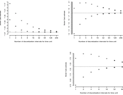
The plots in Figure 1 propose a comparison between E1 and the estimators based on the continuous Euler scheme (E2) and on the discrete Euler scheme (E3). In particular, given a Monte Carlo sample sufficiently large (106), for dif-ferent choices of the starting pointy0and the barriers’ values aandb, we have computed the estimates ofE1 (dotted line) and the estimates produced by E2 andE3 for different discretization intervals. Then we have plotted the values
ofE2 (cross) andE3 (circle) versus the number of discretization intervals.
As we expected, the values of E2 and E3 converge to E1 as the number of discretization interval increases. Indeed it was shown by Gobet (2000) that, for killed diffusions, the weak approximation error of Euler schemes decreases to 0 as the number of discretization intervals increases. When the Monte Carlo sam-ple size is large enough, Monte Carlo error is negligible and the estimated values are affected mainly by the discretization error. In this context the distance be-tween the values of E2 and E3 and the dotted line is a good representation of the (weak) discretization error affecting the Euler schemes and their conver-gence to the dotted line reflects the theoretical converconver-gence of the corresponding expected values. Furthermore, according to the conclusions of Gobet, we notice that the estimates based on the continuous Euler scheme show better conver-gence than the estimates based on the discrete Euler scheme.
both an empirical and a theoretical point of view.
In practical applications, there is an interest in the comparison between the computational times of the Exact Monte Carlo method and the Euler-based methods. However such comparison is not straightforward since Euler schemes are subjected to a trade-off between computational time and discretization error: i.e, as the estimates ofE2 andE3 converge to the dotted line, the time needed to produce them increases. In each plot of Figure 1, we have marked with solid line those values ofE2 andE3 whose computational time was greater than the computational time needed for the estimate ofE1. In these cases our algorithm is both more accurate and more efficient.
6
Conclusions
In this paper we have developed and implemented a novel Monte Carlo method for the estimation of the expected value of a class of functionals of diffusion processes. In particular we considered functionals involving barriers. In these cases the estimation of the expected value is typically challenging. In fact, it is common practice to discretize the underlying diffusion and run Monte Carlo simulation on the discretized process. This clearly introduces a bias in Monte Carlo simulation. Such bias can be reduced only at the cost of a larger computa-tional effort. In comparison, our method turns out to be unbiased and efficient as our simulation study for the sine model demonstrated.
The application of the Exact Algorithm to the multidimensional case is limited to unit diffusion coefficient SDEs whose drift can be expressed as the gradient of a potential (Langevin-type diffusions) (Beskos et al., 2007). In this context the Exact Algorithm returns a Skeleton that gives rise to a factorization of the conditional process in term of the product of multidimensional independent Brownian bridges. For rectangular “killing” regions, a straightforward Multi-variate Exact Monte Carlo algorithm for the barrier problem can be constructed by simulating the crossing events for each of the components of the Brownian bridges. For more general killing regions, the simulation of crossing events of the Brownian bridges is a challenging and open problem. Interesting proposals in this direction can be found in L´epingle (1995), Gobet (2001) and Bossy et al. (2004) for the related problem of the approximation of a reflected multidimen-sional diffusion.
The methodology presented in this paper suggests several further developments and ideas for future research.
We have concentrated here on the (Monte Carlo) barrier problem. This is es-pecially relevant in option pricing for the evaluation of barrier and lookback options and in credit risk modeling for the evaluation of defaultable derivatives. However we believe that there is a wide range of other relevant Monte Carlo problems arising in finance to which the Exact Monte Carlo framework can be successfully applied. For instance current work involves Monte Carlo estimation of the Greeks.
Appendix 1
Brownian bridge two-sided crossing probability (proof of Proposition 1):
LetW be the standard Brownian motion and W(s,x;t,y) be the (s, x)→ (t, y) Brownian bridge. It is well known that, for anyδ > 0:
Wu(0,x;δ,y) d =x+u
δ(y−x) + δ√−u
δ Wδ−uu; 0≤u≤δ
from which we can derive:
pW(s, x;t, y;l1, l2) =P r[l1(u)< Wu< l2(u), u≥0]
where we have set
l1(u) := √l1−y t−su+
l1−x
√ t−s
l2(u) := √l2−y t−su+
l2−x √
t−s
Now, under the usual convention that inf{∅} = ∞, we define the following stopping times:
τ∗= inf{u≥0 :Wu≤l1(u) orWu≥l2(u)}
and
τj,1 = inf{u≥τj−1,2:Wu≤l1(u)}
τj,2 = inf{u≥τj−1,1:Wu≥l2(u)} (j= 1,2, . . .)
under the conventionτ0,1=τ0,2= 0. Let us define the following related events:
A := {τ∗ <∞}
A1 := {τ1,1< τ1,2}; A2:={τ1,2< τ1,1} Aj,n := {τj,n<∞} (j= 1,2, . . .;n= 1,2)
Anderson, 1960, Theorem 4.1) that for anyj∈N:
P r(A2j−1,2) = pj(s, x;t, y;δ, l2); P r(A2j−1,1) =pj(s, x;t, y;δ, l1) P r(A2j,2) = qj(s, x;t, y;δ, l2); P r(A2j,1) =qj(s, x;t, y;δ, l1)
withδ=l2−l1. Straightforward probabilistic arguments lead to the following results:
(i) {Aj,1} ↓ ∅; {Aj,2} ↓ ∅
(ii) A=A2A1=A1,2∪A1,1
(iii) A2=+j=1∞(A2j−1,2−A2j,2) ;A1=+j=1∞(A2j−1,1−A2j,1)
(iv) for anyj= 1,2, . . . : Aj,2∩Aj,1=Aj+1,2∪Aj+1,1
where with the symbolwe denote the disjoint union. Finally we can write:
qW(s, x1;t, x2;l1, l2) = P r(A) =P r(A2) +P r(A1)
= +∞
j=1
[(P r(A2j−1,2)−P r(A2j,2)) + (P r(A2j−1,1)−P r(A2j,1))]
= +∞
j=1
[Pj(s, x;t, y;l1, l2)−Qj(s, x;t, y;l1, l2)]
= lim
k→∞nk(s, x;t, y;l1, l2)
where we have used (ii) and (iii). From (i), for anyj= 1,2, . . .
P r(A2j−1,2)−P r(A2j,2) +P r(A2j−1,1)−P r(A2j,1)≥0
so that{nk}k=1,2,...is increasing, proving (15). On the other side, from (ii) and (iv), the sequence{nk}k=1,2,... (14) can be written in the following way:
n1(s, x;t, y;l1, l2) = P r(A1,2∪A1,1) +P r(A1,2∩A1,1) = P r(A) +c1=q∗(s, x;t, y;l1, l2) +c1 nk(s, x;t, y;l1, l2) = nk−1(s, x;t, y;l1, l2) + (ck−ck−1)
= P r(A) +ck=qW(s, x;t, y;l1, l2) +ck
where{ck =P r(A2k−1,2∩A2k−1,1)}k=1,2,...is decreasing such that limk→∞ck= 0. Therefor for anyk= 1,2, . . .
and
lim
k→+∞nk(s, x;t, y;l1, l2) =P r(A) + limk→∞ck=P r(A) =q
W(s, x;t, y;l
1, l2)
so that (16) follows.
Appendix 2
Let us recall from Beskos and Roberts (2005) conditions 1-3 (C1-C3) for the construction of the Exact Algorithm 1:
C1 The drift functionαis everywhere differentiable
C2 RexpA(u)−u2/2TduwithA(u) =0uα(z)dzis bounded by a constant
C3 The function (α2+α)/2 is bounded
ConditionsB1-B2 in Section 2 trivially impliesC1-C3 if the following Lemma holds.
Lemma 1
Suppose thatαis aC1function onR. Ifα+α2is bounded, then so isα Proof:
Suppose to the contrary, then either:
(i) lim supx→+∞α(x) = +∞
(ii) lim infx→+∞α(x) =−∞
or, alternatively, (i) or (ii) hold withx→ −∞. Firstly, suppose that (i) holds. Then there exists a sequence {xi} → +∞ with {α(xi)} → +∞. Under the hypothesis of the Lemma, for all large enough indecesi, we have:
1. xi >0
2. α(xi)<0
3. α(xi)> α(0)
Since the derivative function α is continuous, by the intermediate value the-orem, there exists yi ∈ [0, xi] such that α(yi) = 0 and α(yi) > α(xi). Thus
{α(yi)} →+∞and α(yi) +α2(yi) =α2(yi) is unbounded ini for a contrad-diction.
Secondly, suppose instead that (ii) holds. Then there exists{xi} →+∞with
1. xi >0
2. α(xi)<0
3. α(y)<0 for ally > xi(otherwise there will be somewhere whereα(y) = 0 leading to a contraddiction similar to in (i))
Therefore, for sufficiently largex, α(x) is decreasing so that limx→+∞α(x) =
−∞. This, combined with the boundedness of the function α +α2, implies that, for any∈(0,1), there existsx0() such that for anyx≥x0 we have:
−
1 α(x)
+= α
(x)
α2(x)+≤0
Choosing = 1/2 and applying the mean value theorem to the continuous functionα, we obtain for anyx≥x0(1/2) andy∈(0, x):
1 α(x)−
1 α(y) ≥
x−y 2
leading to a contradiction.
References
Anderson, T. W. (1960). A modification of the sequential probability ratio test to reduce the sample size. Ann. Math. Statist., 31:165–197.
Asmussen, S. and Glynn, P. W. (2007). Stochastic Simulation. Algorithms and
Analysis. Springer-Verlag, New York. Forthcoming.
Bertoin, J. and Pitman, J. (1994). Path transformations connecting Brownian bridge, excursion and meander. Bull. Sci. Math., 118(2):147–166.
Beskos, A., Papaspiliopoulos, O., and Roberts, G. O. (2006a). Retrospec-tive exact simulation of diffusion sample paths with applications. Bernoulli, 12(6):1077–1098.
Beskos, A., Papaspiliopoulos, O., and Roberts, G. O. (2007). A new factorisation of diffusion measure and sample path reconstruction. Submitted.
Beskos, A., Papaspiliopoulos, O., Roberts, G. O., and Fearnhead, P. (2006b). Exact and efficient likelihood based inference for discretely observed diffusions (with discussion). J. R. Stat. Soc. Ser. B Stat. Methodol., 68(3):333–382.
Beskos, A. and Roberts, G. O. (2005). Exact simulation of diffusions. Ann.
Black, F. and Cox, J. C. (1976). Valuing corporate securities: some effects of bond indenture provisions. Journal of Finance, 31:351–367.
Bossy, M., Gobet, E., and Talay, D. (2004). A symmetrized Euler scheme for an efficient approximation of reflected diffusions.J. Appl. Probab., 41(3):877– 889.
Davydov, D. and Linetsky, V. (2001). The valuation and hedging of barrier and lookback options under the cev process. Management Science, 47:949–965.
Devroye, L. (1986). Nonuniform random variate generation. Springer-Verlag, New York.
Doob, J. L. (1949). Heuristic approach to the Kolmogorov-Smirnov theorems.
Ann. Math. Statistics, 20:393–403.
Fearnhead, P., Papaspiliopoulos, O., and Roberts, G. O. (2006). Particle filters for partially observed diffusions. Submitted.
Gobet, E. (2000). Weak approximation of killed diffusion using Euler schemes.
Stochastic Process. Appl., 87(2):167–197.
Gobet, E. (2001). Euler schemes and half-space approximation for the simulation of diffusion in a domain. ESAIM Probab. Statist., 5:261–297 (electronic).
L´epingle, D. (1995). Euler scheme for reflected stochastic differential equations.
Math. Comput. Simulation, 38(1-3):119–126. Probabilit´es num´eriques (Paris,
1992).
Lerche, H. R. (1986). Boundary crossing of Brownian motion, volume 40 of
Lecture Notes in Statistics. Springer-Verlag, Berlin. Its relation to the law of
the iterated logarithm and to sequential analysis.
Longstaff, F. A. and Schwarz, E. S. (1995). A simple approach to valuing risky and floating rate debt. Journal of Finance, 50:789–819.
Merton, R. C. (1973). Theory of rational option pricing. Bell Journal of
Eco-nomics and Management, (4):141–183.
Oksendal, B. K. (1998). Stochastic Differential Equations: An Introduction
With Applications. Springer-Verlag.
P¨otzelberger, K. and Wang, L. (2001). Boundary crossing probability for Brow-nian motion. J. Appl. Probab., 38(1):152–164.
Number of discretization intervals for time unit
Monte−Carlo estimate
−1.37
−1.33
−1.29
−1.25
−1.21
−1.17
1 2 4 8 16 32 64 128 256
Number of discretization intervals for time unit
Monte−Carlo estimate
1.2
1.3
1.4
1.5
1.6
1.7
1.8
1.9
2
2.1
1 2 4 8 16 32 64 128 256
Number of discretization intervals for time unit
Monte−Carlo estimate
1 2 4 8 16 32 64
0.73
0.93
1.13
1.33
1.53
1.73
[image:26.595.97.504.216.532.2]1.93
Figure 1: Monte Carlo estimates of νfor the model (34) based on the Exact Monte Carlo (dotted line), on the discrete Euler scheme (circle) and on the continuous Euler scheme (cross). Monte Carlo estimates based on the Euler schemes are associated with the corresponding number of disretization intervals. Monte Carlo sample size: 106. Plot 1(top-left): y0 = 0, b= 3, T= 5. Plot 2(top-right): y0= 1.5, b= 4.5, T = 5. Plot 3(bottom-left): y0= 0, a=