State Save Overhead Reduction Techniques for Shared Accelerators in an MPSoC with a Ring NoC

MASTER THESIS

STATE-SAVE

OVERHEAD

REDUCTION

TECHNIQUES FOR

SHARED

ACCELERATORS IN

AN MPSOC WITH A

RING NOC

Oscar Starink

DEPARTMENT OF ELECTRICAL ENGINEERING, MATHEMATHICS AND COMPUTER SCIENCE

COMPUTER ARCHITECTURES FOR EMBEDDED SYSTEMS

EXAMINATION COMMITTEE

University of Twente

Master Thesis

State-Save Overhead Reduction

Techniques for Shared

Accelerators in an MPSoC with a

Ring NoC

Author:

Oscar Starink

Student number:

S1378694

Committee:

Prof. dr. ir. Marco Bekooij

Dr. ir. Jan Broenink

Ir. Guus Kuiper

Research Group Computer Architecture for Embedded Systems,

Department of EEMCS

University of Twente, Enschede, The Netherlands

Abstract

In the last decade chip manufactures moved from single core designs to multi-core designs. This trend is a result of the increasing demand for performance, and the increasing availability of chip area. The same trend is visible in the embedded domain. As a result, System-on-Chips (SoCs) are becoming Multi-Processor System-on-Chips (MPSoCs). These multi-processor systems can be homogeneous or heterogeneous. In a homogeneous system all processors are identical, while a heterogeneous system contains multiple different processing elements. A processing element can perform a general or a specific task. A Central Processing Unit (CPU) is an example of a general purpose processing element, while a hardware accelerator is an application specific processing ele-ment. The MPSoCs also contain a Network-on-Chip (NoC) that is connecting all the processing elements within an MPSoC.

Researchers at the University of Twente have developed an MPSoC, that targets real-time streaming applications. It started as a homogeneous MPSoC with an NoC that can give real-time guarantees about the traffic, and has grown into a heterogeneous MPSoC. By adding hardware accelerators the architecture could deliver more performance.

The hardware accelerators have enough performance to process multiple data streams, but the architecture was not capable of sharing a hardware accelerator over multiple streams. So multiple hardware accelerators were needed, one for each stream. This was solved by introducing a centralized component called the gateway. The gateway orchestrates the sharing of an accelerator by multiple data streams. This is done by processing a block of data from one stream, and then a block of data from an other stream. A case study showed that the gateway could correctly enable sharing of an accelerator by multiple streams, but the utilization of the accelerators was low, due to the so called state-save overhead. Because the accelerators contain state, the gateway must save and restore this state when a switch is made between data streams. This thesis is focused on determining the causes of the high state-save overhead and the definition and evaluation of techniques that reduce this overhead.

ring network to support state being streamed from and to the accelerators. The proposed architecture is implemented and a dataflow model is proposed that corresponds to the new architecture. With this dataflow model it is possible to determine some real-time properties of the system.

Acknowledgements

First of all I would like to thank Marco for his supervision and feedback during my thesis. I really admire his determination to explore new areas, and his enthusiasm that is an inspiration for others to become explorers.

I would also like to thank Guus, Berend and Gerben. They helped me get started with the Starburst architecture and were always willing to help or answer the questions that I had.

Additionally I would like to pay my tribute to all the CAES member, for several memorable discussions during the coffee breaks and Friday afternoon drinks. Finally I would like to thank Tristia, for her support and motivation during my thesis.

Oscar Starink

Contents

Abstract i

Acknowledgements iii

Contents iv

List of Figures vi

List of Tables vii

List of Acronyms viii

1 Introduction 1

1.1 Context . . . 1

1.2 Research Platform . . . 2

1.2.1 Accelerator Sharing Architecture . . . 2

1.2.2 Dataflow Modelling . . . 3

1.3 Problem Description . . . 4

1.4 Research Questions . . . 5

1.5 Contributions . . . 6

1.6 Outline . . . 6

2 Related Work 8 2.1 Hardware accelerators . . . 8

2.1.1 Instruction set extension . . . 9

2.1.2 Remote procedure call . . . 9

2.1.3 Stream based hardware accelerator . . . 9

2.2 Accelerator sharing architectures . . . 10

2.2.1 Context switch . . . 10

2.2.2 PROPHID . . . 11

2.2.3 Eclipse . . . 11

2.2.4 Starburst . . . 12

2.3 Real-time analysis techniques . . . 13

2.3.2 Real-time calculus . . . 13

2.3.3 Synchronous dataflow . . . 13

2.4 Modelling accelerator sharing . . . 14

3 Implementation 15 3.1 Previous accelerator sharing implementation . . . 15

3.1.1 Hardware . . . 15

3.1.2 Software . . . 18

3.1.3 Pinpointing the problem . . . 18

3.2 Basic idea . . . 19

3.3 Proposed implementation . . . 20

3.3.1 Hardware . . . 20

3.3.2 Software . . . 25

3.3.3 Restore-save sequence . . . 27

4 Dataflow Analysis 30 4.1 Previous Accelerator Sharing Models . . . 30

4.2 Proposed CSDF model . . . 32

4.3 Proposed SDF model . . . 34

5 Evaluation 37 5.1 The benchmark application . . . 37

5.2 Evaluation of the implementation . . . 39

5.2.1 Speed . . . 39

5.2.2 Size . . . 41

5.3 Evaluation of the dataflow models . . . 43

5.3.1 Throughput . . . 43

5.3.2 Buffer size . . . 44

5.3.3 Packet size . . . 44

6 Conclusion and Future Work 45 6.1 Conclusion . . . 45

6.2 Future Work . . . 46

6.2.1 Stack machine entry gateway . . . 47

6.2.2 Nebula ring topology . . . 48

6.2.3 Evaluation of dataflow models . . . 50

List of Figures

1.1 Global system overview . . . 2

1.2 Dataflow model of a shared accelerator . . . 4

1.3 Abstracted dataflow graph of Figure 1.2 . . . 4

3.1 High level system overview . . . 16

3.2 Nebula ring network connection . . . 17

3.3 High level overview of the proposed architecture . . . 21

3.4 Nebula ring network connection with RWI . . . 22

3.5 Modes of the RWI and the possible transitions . . . 24

3.6 Transfers and RWI modes during restore stage . . . 28

3.7 Transfers and RWI modes during process stage . . . 28

3.8 Transfers and RWI modes during save stage . . . 29

4.1 Previous CSDF model . . . 31

4.2 Previous SDF model . . . 32

4.3 SDF models of the different accelerator behaviours . . . 33

4.4 CSDF model of an accelerators restore-save cycle . . . 33

4.5 Proposed CSDF model . . . 34

4.6 Typical schedule of the CSDF model . . . 35

4.7 Proposed SDF model . . . 36

5.1 Stereo FM demodulation block diagram . . . 38

5.2 High level system overview used for evaluation . . . 38

5.3 Throughput comparison . . . 39

5.4 Utilisation comparison . . . 40

5.5 Hardware cost for individual components . . . 42

5.6 Hardware cost comparison . . . 43

6.1 Alternative entry gateway architecture with a J1 CPU . . . 47

List of Tables

List of Acronyms

ACC ACCelerator.

ADS Application Domain Specific.

AXI Advanced eXtensible Interface.

CORDIC COordinate Rotation DIgital Computer.

CPU Central Processing Unit.

CSDF Cyclo-Static DataFlow.

DDR3 Double Data Rate type 3.

DMA Direct Memory Access.

EGW Exit GateWay.

FIFO First In, First Out.

FIR Finite Impulse Response.

GW entry GateWay.

ISE Instruction Set Extension.

LUT Look-Up Table.

LUTRAM LUT used as RAM.

MPSoC Multi-Processor System-on-Chip.

NoC Network-on-Chip.

OS Operating System.

PLB Processor Local Bus.

RAM Random Access Memory.

RWI Read/Write Interface.

SDF Synchronous DataFlow.

SoC System-on-Chip.

USB Universal Serial Bus.

Chapter 1

Introduction

1.1

Context

For the last decades the number of transistors on a chip grew exponentially. This made enormous advances in CPUs possible. Where one of the first CPUs had several thousand transistors, the latest CPUs consist of several billion tran-sistors.

These developments are driven by the demand for more computational perfor-mance. There is not only a demand for powerful personal computers in the consumer market, also embedded systems found in video and radio applications continue their demand for more computational performance. Advances in decod-ing, decompression and software defined radio algorithms are big contributors to this demand.

In order to cope with the demand, chip manufacturers started to create MP-SoCs. These architectures can make use of the many transistors that are avail-able by placing and connecting multiple processors. Performance is delivered by the parallel capabilities of the architecture. One can divide MPSoCs into two categories, homogeneous and heterogeneous. A homogeneous architecture consists of multiple identical processors, while heterogeneous architecture con-sists of multiple different processors. These heterogeneous architectures often add hardware accelerators that can only perform one specific computation. The advantage of these accelerators is that they can perform these computations effectively in terms of speed and energy.

its users and also needs a scheduling policy. Hardware architectures capable of sharing accelerators is a relatively new research area.

Mapping applications on parallel hardware is not always an easy task, and a lot of research is done is this area. This thesis will look at streaming applications. Streaming applications typically operate on an input stream and compute the output stream. These applications can often be mapped elegantly on parallel hardware.

Streaming applications usually have real-time requirements. This means that correctness not only depends on the computed result, but also on the time when results are produced. In order to guarantee correct temporal behaviour, models can be used to check temporal correctness. Developing models and modelling techniques is an actively researched area.

1.2

Research Platform

This section will give the background needed to understand and formulate the problem description. The first subsection contains a high level overview of an architecture that can share its accelerators. We will call an architecture capable of this an accelerator sharing architecture. The second subsection will introduce the models that are used to analyse the accelerator sharing architecture.

1.2.1

Accelerator Sharing Architecture

In this subsection we will present a heterogeneous MPSoC architecture that is suitable for streaming applications and capable of accelerator sharing. This architecture is first introduced in [1].

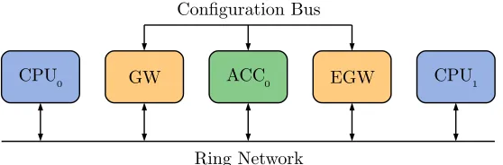
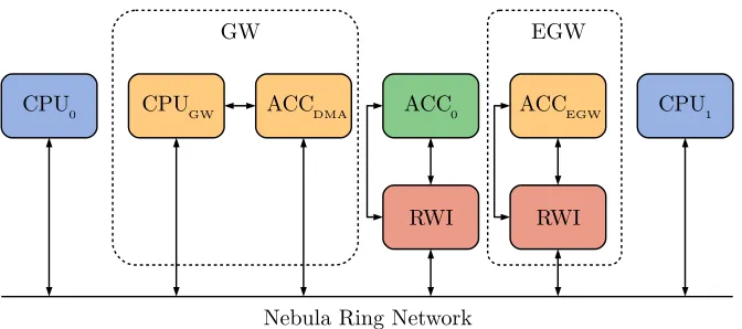
CPU₀ GW ACC₀ EGW CPU₁

Ring Network Configuration Bus

Figure 1.1: Global system overview

A CPU tile is connected to the ring network in order to communicate with other tiles. CPU tiles can be used for general computations.

An accelerator tile is a specialized component that can perform a specific op-eration efficiently. For example a Finite Impulse Response (FIR) filter. The accelerator tiles are also connected to the ring network. Additionally they have a configuration interface, which is connected to the configuration bus. An ac-celerator has an internal state that must be saved and restored when switching between two streams, the configuration bus is used for this.

Then there are the gateway tiles that have a specific function. The entry Gate-Way (GW) is responsible for the coordination of the sharing of the accelerators. When a block of data is received from a producer by the entry gateway, it will configure and restore the state of the accelerators using the configuration bus. Then it will send the data block to the accelerators, via the ring network. When the accelerators have processed the data the entry gateway will save the state of the accelerators, again using the configuration bus.

After the last accelerator in the accelerator chain comes the Exit GateWay (EGW). This tile is used to write the data to the correct consumer CPU. It is also used to check if all the data elements are processed by the accelerators. Because only then a state-save can be performed.

Placing an entry and exit gateway around an accelerator chain, makes it possible to share the accelerators in a transparent way. The gateway pair will ”hide” the accelerator sharing for the producer and consumer.

1.2.2

Dataflow Modelling

In order to guarantee temporal constraints of an architecture, models are used that capture the temporal behaviour of the architecture. In this subsection we will discuss two dataflow models that capture the temporal behaviour of the accelerator sharing architecture, that were introduced in [2]. The first model is directly derived from the architecture. The second model is an abstraction of the first model.

For now only simplified dataflow models are presented. These are only used to illustrate some basic concepts. This subsection should be readable without expert knowledge about dataflow modelling.

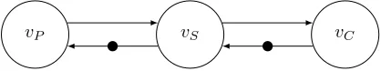
Figure 1.2 shows the first model. It shows 5 actors connected with each other by edges. The actors have a one-to-one relation with the architecture. The actor

vP is the producing CPU,vG is the entry gateway,vAis an accelerator, vEGis

the exit gateway andvC is the consuming CPU.

The edge fromvEG to vE represents the signal from the exit gateway to the

entry gateway that indicates that all data is processed and the accelerators can be reconfigured. So reconfiguration is postponed until all data is out of the accelerator chain. This is called a pipeline flush. Flushing a pipeline has a performance penalty, because the pipeline is no longer constantly utilised.

vP vG vA vEG vC

Figure 1.2: Dataflow model of a shared accelerator

Another basic concept is abstraction of dataflow models. This is a useful tech-nique that can be applied on a complex model, in order to reduce its complexity. Figure 1.3 shows an abstraction of the model in Figure 1.2. ActorvG, vA and vEGand the edges between them are abstracted intovS.

An abstraction can be used to reduce the complexity which can make reasoning about the model simpler. However by removing details, the model can become less accurate and will likely be an over approximation of the original model. An abstraction is done in such a way that some properties that hold for the abstraction also hold for the original model.

vP vS vC

Figure 1.3: Abstracted dataflow graph of Figure 1.2

1.3

Problem Description

Sharing accelerators has its advantages, but it also introduces some problems. This section will highlight those problems.

As mentioned in the previous sections accelerator sharing has its advantages. The accelerators will be better utilized and sharing an accelerator reduces the hardware. However there are disadvantages as well. Sharing an accelerator requires synchronisation of its users, and it can result in all kinds of synchro-nisation problems, like deadlock and race conditions. Another disadvantage is that these synchronisation have some overhead. However this overhead is relatively small, and thus acceptable.

acceler-ator sharing, it handles all synchronisation and schedules the requests. This makes development of applications easier, because producers and consumers only connect to the gateway and are not aware of other computations on the accelerators.

The biggest problem is state. Most of the accelerators have an internal state that is needed for the computation. For instance the previous samples are needed in the computation of an FIR filter. As two different computations most likely have different states, the state must be saved and restored between computations. This will introduce some overhead, which is called state-save overhead. The size of the state-save overhead depends on how the state is saved. The state-save overhead prevents full utilization of the accelerators. In order to reduce a large state-save overhead ratio, computations are made longer. So context switches will occur less often. This will increase the through-put of an application. But when a task processes more data, it will delay the start of the other tasks because they are sharing the accelerator. So when more data is processed between switches, it results in a higher latency and larger data bursts. In order to cope with larger data burst, larger buffers are necessary. So there exist a trade off with on one hand throughput and on the other buffer size and latency.

State-saves in the architecture described in Section 1.2 are done by copying the state to the memory in the gateway. This means that the state-save overhead is linearly related to the state size. Measurements on the architecture indicate that the state-save overhead is relative high, 23 clock cycles per 32-bit word transfer [1]. In this thesis we will describe a technique to reduce the state-save overhead.

In order to analyse the temporal behaviour, there must be a dataflow model of the proposed architecture. It is likely that a different dataflow model is needed when the hardware is modified to reduce the state-save overhead. If this is the case also an abstraction should be made, in order to simplify the new dataflow model. Furthermore the improvements of the new architecture should be reflected in the new dataflow models.

1.4

Research Questions

The goal of this research is to answer the following research question:

How to reduce state-save overhead for shared accelerators in an MP-SoC with a ring NoC?

proper-ties should be quantified by means of measured results. From these objectives the following sub-questions are derived:

• What is the cause for the large state-save overhead?

• Is it possible to introduce an architecture that reduces the state-save over-head?

• What is the performance of this architecture?

• What is the hardware cost of this architecture?

• Is it possible to model the temporal behaviour of the architecture?

• Do the models capture the gain in performance?

1.5

Contributions

In this thesis we describe improvements of an architecture capable of sharing accelerators [1] and their corresponding dataflow models [2]. The main contri-butions described in this thesis are:

• Pinpointing the cause of the large state-save overhead in the existing ac-celerator sharing archtecture [1].

• The proposal of an architecture capable of sharing accelerators that has lower state-save overhead.

• Description of the implementation of the proposed architecture.

• Proposing dataflow models for the architecture.

• Evaluation of the architecture and the dataflow models.

1.6

Outline

Chapter 2

Related Work

In this chapter we will discuss work related to state-saving for shared acceler-ators. First we will discuss some methods to include accelerators in an archi-tecture. Next we discuss a number of accelerator sharing architectures. In the third part we will discuss multiple real-time analysis techniques. Finally we mention a technique to model shared accelerators.

2.1

Hardware accelerators

In this section we will discuss the advantages and disadvantages of hardware accelerators and how they can be integrated into a system.

In systems that perform calculations there is typically a trade-off between effi-ciency and flexibility. It is often the case that flexible systems are not as efficient as their static counter part.

2.1.1

Instruction set extension

One technique to combine CPUs and hardware accelerators is via an Instruction Set Extension (ISE). The CPU is designed to have some additional instructions that are used to control the hardware accelerator. This results in a tight coupling of the CPU and accelerator. Examples of these ISEs are the MMX and SSE extensions in the x86 processor architectures.

Our architecture does not use ISEs to control the hardware accelerators, because this technique prevents sharing of the accelerator, due to the tight coupling of the CPU and accelerator.

2.1.2

Remote procedure call

Another way to control hardware accelerators is via Remote Procedure Calls (RPCs). RPCs enable a CPU to start a calculation somewhere else in the system. Typically the CPU and accelerators are connected via a bus and the RPCs are performed by reads and writes. An example of this technique is the IBM 4764 PCI-X Cryptographic Coprocessor [3]. This is a hardware accelerator that can be used for cryptographic calculation. It is connected via the PCI bus which is a common bus in computers.

While it is possible to share the accelerators with this technique, we do not use RPCs in our architecture because it is not possible to cascade the result of a cal-culation to another accelerator. This is a disadvantage because our architecture targets streaming applications, where the ability to chain accelerators can be a real advantage. Also when a RPC is performed the CPU has to wait for the result. This time is lost, since the CPU cannot perform any useful calculations while it wait. When stream based hardware accelerators are used the CPU only has to write a data stream to the accelerator. The CPU does not have to wait on the result, because this stream will typically go to an other consumer. Because the CPU does not have to wait, it can perform more useful calculations.

2.1.3

Stream based hardware accelerator

The stream based hardware accelerators perform calculations on streams. The CPUs are used to produce and consume data streams that can be processed by accelerators. A good example of this technique is the Starburst architecture [4]. CPUs and accelerators are connected via the Nebula ring network which has support for stream based communication [5].

2.2

Accelerator sharing architectures

In this section we will discuss several accelerator sharing architectures that are related to the accelerator sharing techniques presented in this thesis. First we will describe context switches that are used by Operating Systems (OSs) to share the CPU over multiple programs. After this we will describe the PROPHID and Eclipse architectures that are both capable of accelerator sharing.

2.2.1

Context switch

The accelerator sharing techniques in this thesis have a lot in common with the context switches performed by modern OSs such as Windows and Linux. These context switches make it possible for multiple programs to share the same CPU. This looks a lot like multiple data streams that share the same accelerator. Just as an accelerator the CPU has an internal state, due to the general-purpose registers and status flags. The state needs to be saved, so it can be restored later. The saving and restoring of the state is done within a context switch. During a context switch the state of the CPU is stored into memory. Then it will determine which program will be continued. The CPU state corresponding to that program is loaded from memory and restored. Now the program can continue its execution. Typically context switching is done periodically by a timer interrupt. This will interleave the executions of the different programmes, giving the illusion that they are running in parallel.

Similarities with our techniques are that the state is saved into memory and restored on a later moment. Another similarity is that both approaches result in interleaving. Furthermore they both have some overhead that is due to the saving and restoring. A difference is that the context switch is performed by the CPU itself, while we initiate the saving and restoring from the gateway. Another difference is that the CPU performing the context switch is directly connected to memory. This is in contrast with the accelerator, which has no access to memory. Instead the state is retrieved by the gateway and saved into memory of the gateway. Lastly the context switching is done periodically, while the gateway switches streams after a fixed number of data samples, this is called the packet size. We can say that the task that share an accelerators are cooperatively scheduled, because after the packet size the running task allows other task to run. So there are aware that the accelerator is shared, and give the other tasks also a chance to use the accelerator. While tasks that share a CPU are typically pre-emptively scheduled, this means that the tasks are not aware that the CPU is shared. The context switch interrupts a running task and pauses it, while a task that was paused will be continued.

the overhead becomes bigger and the responsiveness increases if the packet size is decreased. An appropriate packet size depends on the application.

2.2.2

PROPHID

PROPHID [6] is a heterogeneous multiprocessor architecture that is designed to deliver guaranteed real-time processing for multimedia applications. The archi-tecture consists of two main parts. The first is one CPU that is primarily used for control oriented tasks and the second part consists of multiple Application Domain Specific (ADS) processors that perform the high performance and time critical operations. The CPU and ADS processors are connected to a central bus. The ADS processors are also connected to a programmable high bandwidth communication network. There is a main memory which can be accessed from the central bus and from the communication network via an arbiter.

In order to improve the utilization of the ADS processors, they are capable to process between 1 and 5 data steams in a time interleaved fashion. The ADS processors have multiple input and output First In, First Outs (FIFOs), equal to the number of streams it supports. Context switches are done at a fine granularity, in order to keep the FIFOs sizes small, because FIFOs can typically hold only 32 samples. The ADS processors also have multiple state banks, equal to the number of streams it supports. These state banks make context switches almost instant, this is the reason that fine granularity is possible without a large state-save overhead.

There are a lot of similarities between PROPHID and our architecture. Both al-low hardware accelerators to be shared over multiple streams and consequently, both perform state-saves. A difference is that ADS processors have additional hardware and local memory to perform the state saving and restoring. This means that the maximum number of streams is determined by the number of states the local memory can hold. Another difference is it that the CPU is not connected to the high-throughput network and cannot be used to process data streams. While in our architecture the CPUs are connected to the ring network and they can be used to process data streams.

2.2.3

Eclipse

The 5 primitives are GetTask, Read, Write, GetSpace and PutSpace [7]. A coprocessor gets a task ID together with optional configuration data with the

GetTaskprimitive. The task ID is used as identifier for the different task, and

is used as an argument for all other primitives. Then it needs to reserve free space in the destination FIFO and check for data in the source FIFO. This is done with theGetSpace primitive. If there is no data in the source FIFO or no free space in the destination FIFO, it cannot perform the current task and it will request a new task. If it is possible to continue it will read the source FIFO with the Read primitive. This is followed by the PutSpaceprimitive to indicate that the data is read. The coprocessor can now start its computation. The results are stored with theWriteprimitive and followed with thePutSpace

primitive to indicate that there is new data. Now the coprocessor can start with a new task.

Eclipse and our architecture have some similarities. Computations can be done by a mix of processors and coprocessors and communication between tasks is done with FIFOs. A difference is that Eclipse provides a uniform interface to the network for processors and coprocessors via its shell primitives. However these high level primitives result in large hardware costs of the shells. In our architecture the processors and accelerators have two separate communication mechanisms, resulting in a lower hardware cost. Another difference is that each coprocessor needs a shell, in our architecture multiple accelerators can be managed by one entry gateway and exit gateway pair. While the Eclipse is capable of sharing coprocessors, state-saving mechanisms for coprocessors are not described.

2.2.4

Starburst

The Starburst platform is an MPSoC with CPUs and hardware accelerators, that targets streaming applications. The accelerators in this system are stream oriented. The CPUs and accelerators in the system are connected via a ring NoC, that has support for data streams. In [1] the Starburst platform is ex-tended to support sharing of accelerators by introducing an entry and exit gate-way to the system. These gategate-ways can schedule multiple different data streams over the accelerators and it will save and restore the state of the accelerator when this is needed. The state saving and restoring of the accelerators is done via a configuration bus that connects all accelerators to the entry gateway.

2.3

Real-time analysis techniques

Analysis of real-time systems is used to guarantee temporal constrains. There are three major frameworks that can be used to perform real-time analysis. These frameworks are suited to model concurrent application and pipelined execution. We will briefly mention these three techniques.

2.3.1

SymTA/S

The SymTA/S [8] framework is based on event models. In event models the traffic is characterised with a period and a jitter. The traffic characterisation can have low accuracy, because the correlation between different streams is not captured. It does not support cyclic data dependency in the general case because the analysis technique will report that the latency is infinite [9].

2.3.2

Real-time calculus

Real-time calculus [10] is an analysis technique based on network calculus. It characterises the traffic between components in the time domain. Attempts are made to handle cyclic dependencies [11], [12]. Both approaches only consider cyclic data dependencies or cyclic resource dependencies, but not a combination of both.

2.3.3

Synchronous dataflow

Synchronous DataFlow (SDF) [13] [14] is closely related to Kahn networks. SDF operates on directed graphs, where cycles are allowed. Tokens are transported over the edges, and can be used for example to model data or free space in a buffer. The actors have firing durations. When all input edges contain enough tokens, the actor is enabled and after the firing duration the actor will fire. When an actor fires it consumes tokens for the input edges and will produce to-kens on the output edges. The number of toto-kens that is produced or consumed is indicated by the production and consumption quanta. Analysis is done by creating a schedule. This schedule is used to determine minimal buffer sizes and guarantee throughput constrains. Executions of tasks can be specified in multiple ways, for instance using Worst Case Execution Time (WCET) or with a (σ,ρ)-characterisation [15]. Resources can be shared with different schedulers, starvation-free schedulers such as round robin and budget scheduling, and re-cently also non-starvation-free schedulers can be used such as static-priority scheduling [15].

dependencies. Cyclic data dependencies are used to model finite buffers and the sharing of the accelerators result in a cyclic resource dependency. Another motivation is that parts of the proposed architecture already have been modelled with data flow, such as the NoC in [16], and the accelerator sharing architecture presented in [1] has been modelled with dataflow in [2].

2.4

Modelling accelerator sharing

In this section we will discuss related work relevant to the modelling of acceler-ators that are shared.

In [17] SDF and Cyclo-Static DataFlow (CSDF) are used to model the sharing of accelerators. The data streams are scheduled with a round robin scheduler. The models can be used to satisfy minimum throughput constrains for multiple data streams.

Chapter 3

Implementation

This chapter will describe the architectures used for accelerator sharing. The first section will describe the previous architecture and its limitations. Then the basic idea is presented that will deal with the problems. Finally the proposed architecture is described in detail.

3.1

Previous accelerator sharing implementation

In this section the previous accelerator sharing implementation will be shown that was described in [1]. First the hardware of the architecture is presented. After this the software structure will be explained.

3.1.1

Hardware

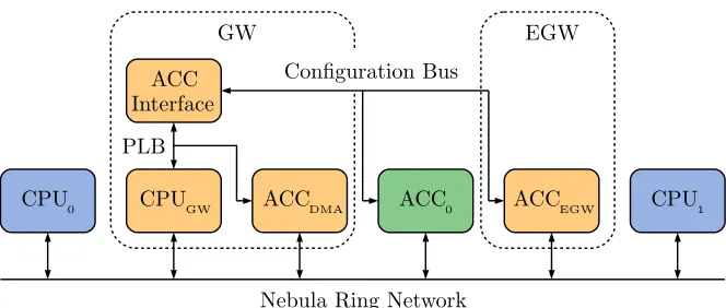
Section 1.2.1 already gave a global overview of the architecture, this subsection will recap Section 1.2.1 and give a more detailed overview of the architecture. The Starburst [4] is heterogeneous MPSoC and consists out of CPUs and ac-celerators. We will use Figure 3.1 to explain all the components of the system. Figure 3.1 shows only a small number of CPUs and accelerators, but a typical system consists out of multiple CPUs and accelerators.

The Nebula ring network [5] connects all the components in the system. The Nebula is an unidirectional, guaranteed-throughput ring network. It uses slots to guarantee that all components that are connected to the ring have a guaranteed-throughput.

CPU₀ CPU₁ ACC

Interface

ACC₀

CPU_GW ACC_DMA ACC_EGW

Nebula Ring Network

EGW GW

Configuration Bus

PLB

Figure 3.1: High level system overview

The accelerators are also connected to the ring network. Additionally they have a configuration interface, which is connected to the ACCelerator (ACC) Interface. The ACC Interface is used to perform the state-saves.

Then there are some components that together have a specific function. The gateway CPU (CPUGW) together with the ACC Interface and accelerator Direct

Memory Access (DMA) (ACCDMA) form the entry gateway. These components

are connected via the Xilinx Processor Local Bus (PLB) bus. The entry gateway is responsible for the coordination of the sharing of the accelerators. When a block of data is received by the entry gateway, it will configure and restore the state of the accelerators using the ACC Interface. Then it will send the data block via the Nebula ring network to the accelerators. This is done with the accelerator DMA, also called Ring DMA. When the accelerators have processed the data the entry gateway will save the state of the accelerators, again using the ACC Interface.

When the design contains multiple accelerators, it is possible to use the out-put of an accelerator as inout-put for another accelerator. When this is done the accelerators form a chain, and we will call this an accelerator chain.

The last accelerator in the accelerator chain is the exit gateway accelerator (ACCEGW), and this forms the exit gateway. This accelerator is used to write

the data to a scratch pad memory of a CPU. It is also used to check if the last data element is processed by the accelerators.

There are components that are not shown because they are of no relevance for the discussion in this thesis. However they will be mentioned here for complete-ness. Every CPU is connected to one global Double Data Rate type 3 (DDR3) memory, with an arbitration tree. There also is one CPU that runs Linux. This CPU has additional peripherals, such as an Universal Serial Bus (USB) and an Ethernet controller.

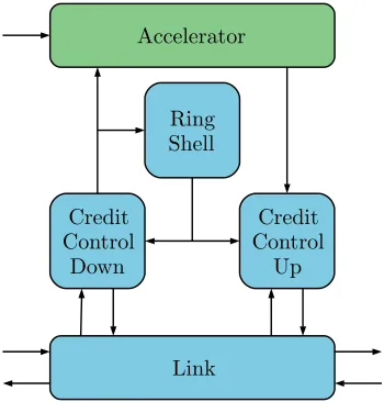
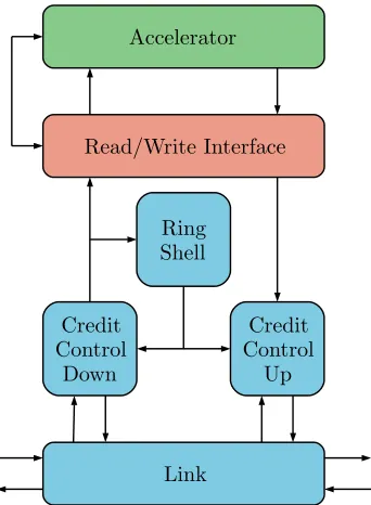
write-only, address based communication to the scratch pad memories. This communication is used by the CFIFOs. CFIFOs logical FIFOs that are imple-mented in software that are based on the C-HEAP [18] algorithm. The CFIFOs are used for communication between CPUs. The other type of communication is credit based. Communication between accelerators is of this type. The credit based communication is designed to have low hardware cost and supports back pressure. The back pressure is needed prevents buffer overflows in the acceler-ator [5]. The sender of data to the acceleracceler-ator is keeping a local counter of free space in the buffer of the accelerator. When the sender sends one data word it will subtract one from the counter. By preventing the sender to send while the counter is zero, a buffer overflow can not occur. When the accelerator consumes a data word from its buffer, a credit is sent to the sender. When the sender receives the credit the counter will be incremented by one. In order to support the credit based communication the Nebula ring network contains additional hardware. Figure 3.2 shows a detailed overview of the additional hardware. Figure 3.2 shows how an accelerator is connected to the ring network. The link performs the most basic operation, it schedules data transfers and credit transfers in the available slots. The credit control down block will buffer received data and when the data is consumed by the accelerator it will generate an acknowledgement credit. The credit control up block keeps a local counter of free space of the next accelerator in the chain, and prevents data to be sent when the local counter is zero. The ring shell is used to configure the destination addresses of the credit and the data. These addresses must correspond with the previous and next accelerator addresses in the chain of accelerators.

Credit Control

Down

Link

Credit Control

Up Ring

Shell Accelerator

3.1.2

Software

The software that runs on the gateway CPU is responsible for the state-saves and state restores. The code is written in C++ _{and uses an object orientated}

approach. For every accelerator there is a corresponding class that can save and restore the state of that accelerator. The class is also responsible for the storage of the state data. Every specific accelerator class inherits from the accelerator base class. This base class contains the data forward and the credit return address. These addresses correspond with the addresses needed in the ring shell in order to have correct credit based communication.

Then there is an AccList object that is used to create accelerator chains. Mul-tiple accelerators can be added to the AccList. The AccList is used to process a block of data with the accelerators, this function is called process and the following will happen. First the data forward and the credit return address are configured for every accelerator in the list. Then for every accelerator the state is restored, by calling the restore function of every accelerator object. Now the data can be sent to the accelerators. The gateway waits until all data is processed by the accelerators. The last thing it does is saving the state of the accelerators, by calling the save function of every accelerator object in the list. The AccList object uses the decorator pattern [19] to represent the structure of the accelerator chain. The template method pattern [19] is used to generate the correct behaviour.

When the accelerators are shared there is more than one AccList object and these objects need to be scheduled. The scheduler will check that there is data available from the producer and that the consumer is ready for new data. If these conditions are satisfied it will call the corresponding AccList process function.

3.1.3

Pinpointing the problem

This subsection pinpoints the cause for the high state-save overhead. As stated before the average time to read or write a 32-bit word of state from an accelerator is 23 processor cycles [1]. After looking into the implementation the following causes for the high state-save overhead were identified.

• Slow state data access over the ACC Interface. The ACC Interface is connected to the CPU via the PLB bus. This bus has a high transfer overhead, when a single transfer is done. This is likely a significant part of the state-save overhead.

• A lot of code in the critical loop. The code that is responsible for saving and restoring the state is located in multiple C++_{objects. So the gateway}

3.2

Basic idea

This section presents approaches to solve the problems that where identified in Section 3.1.3.

• The proposed design will use the Nebula ring network to perform state-saves, instead of the PLB bus. The Nebula ring network is capable to transfer one word each cycle, and thus fast. This will help to reduce the state-save overhead. It would even be possible to use the Ring-DMA to send state to the accelerators. An other advantage is that the ACC Interface can be removed, reducing the hardware cost of the design. In order to be able to send state to the accelerators via the ring network it is necessary to be able to differentiate between data and state. So some additional control logic is needed in order to support this. By placing this control logic between the accelerators and the network, the control logic has full control over the accelerator and is immediately connected to the Nebula ring network. So no additional network connections are needed, and this will keep the hardware cost down. Another advantage of this approach is that most of the hardware already exists and can be reused. This will keep the development time within limits. Reuse of the accelerators is achieved by connecting the control logic to the existing configuration interface of an accelerator. In order to differentiate between state and data, commands will be used to indicate what is being send, state or data. Sending these commands has some overhead, but they are needed to be able to use the Nebula ring network. We expect that the performance gain will outweigh the extra overhead. A disadvantage of this approach is that when the state of an accelerator is saved to the memory in the entry gateway, it will traverse the whole ring network, because the Nebula ring network is unidirectional. For now we will accept this, but in future work section we will present a possible solution to prevent this.

• In order to improve the software that performs the state-saves, we will try to minimize the number function calls and the number of instructions that are executed in the critical loop. Due to the template method pattern the code that performs a restore-save cycle, is located in different C++

perform the restore-save cycle. With this approach it will be possible to have a low code size and only a few function calls in the critical loop, because only the interpreter is executed. This is expected to result in a better performance. Another advantage is that the list of transfers can be optimized. Multiple single transfers to the same address can be optimized to a burst transfer. This allows us to make use of DMA burst transfers, resulting in faster transfers. Because we still use the decorator pattern it is still easy to define the structure of the accelerator chain. A disadvantage of this method is that it uses more memory, because it needs to store the list of transfers. However the embedded system has a large DDR3 memory that can be used so this is not a real problem. Another disadvantage is that once the list of transfers is build, it is no longer possible to add additional accelerators to the processing chain. But most applications do not require dynamic addition of accelerators, so typically this will not be an issue.

3.3

Proposed implementation

This section will present the proposed architecture for accelerator sharing. This section is divided in three subsections. First the hardware is presented. The sec-ond subsection will discus the changes made in the software. The last subsection will discus what the steps are to perform a restore-save cycle.

3.3.1

Hardware

Figure 3.3 shows the top level changes to the architecture shown in Figure 3.1. The ACC Interface is completely removed, and all accelerators that were con-nected to the ACC Interface are now concon-nected to the Nebula ring network via the Read/Write Interface (RWI). The RWI makes it possible to configure the accelerators via the Nebula ring network, this is indicated by the configuration bus connected to the sides of the accelerators and the RWI. Note that the DMA accelerator does not have an RWI. This is because it is still directly connected to the gateway CPU via the PLB bus.

In Figure 3.4 can be seen that the RWI is placed in between the accelerator and the Nebula ring network logic. So using the RWI does not require rigorous changes in the existing hardware.

CPU

0 CPUGW ACCDMA ACC0 ACCEGW CPU1

RWI RWI

Nebula Ring Network

GW EGW

Figure 3.3: High level overview of the proposed architecture

Read/Write Interface

Because the RWI receives both data and state, it needs a way to differentiate between the two. This is done by introducing modes. The RWI has internal modes and the mode dictates if the received words are data or state. The RWI has the following modes: normal, read, write and bypass. What these modes exactly do, will be described in the section RWI modes. First it is discussed how modes are changed. The modes can be altered by sending commands. So now the RWI needs to differentiate between data and commands. This is done by using the address of the data transfer. Table 3.1 shows the meaning of the bits in the address space of the Nebula ring network. Bit 15 is removed from the free address space and is now used to indicate a RWI command.

Bit Meaning

31:28 0x6 is the address space of the Nebula ring network 27:20 CPU ID

19:17 Sub ID, ID 0 is the CPU, other ID’s are accelerators 16 0 for credit based data, 1 for Ringshell access 15 0 for data, 1 for RWI commando

14:0 Free address space

Table 3.1: Meaning of Nebula ring network address bits

Credit Control

Down

Link

Credit Control

Up Ring

Shell

Read/Write Interface Accelerator

Figure 3.4: Nebula ring network connection with RWI

the ID field (bits 31:20) is a match, the mode field (bits 19:18) is used to switch modes. When the mode becomes reading or writing, the address field (bits 11:0) is used to determine the start address, and the number of reads/writes field (bits 17:12) indicates the number of reads/writes.

Bit Meaning 31:20 ID

19:18 Mode, ’00’ normal, ’10’ read, ’01’ write, ’11’ bypass 17:12 Number of reads/writes

11:0 Read/write address

Table 3.2: Meaning of the RWI command data bits

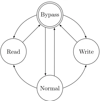
RWI modes

The RWI has 4 modes and Figure 3.5 shows how each mode can be reached. After a reset the RWI will start in bypass mode. Each mode has it own behaviour and these will be explained below.

network. So this is the mode the RWI should be in, when the accelerator is used for processing.

When the RWI is switched to read mode, a start address and the number of reads are set. This mode will read a word via the accelerator configuration bus from the start address and will sent this word to the next accelerator via the Nebula ring network. The number of reads is decreased with one and the start address is incremented to the next word. While the number of reads is not zero it will perform another read cycle. When the number of reads reaches zero, the RWI will switch to the bypass mode.

When the RWI is switched to write mode, a start address and the number of writes are set. This mode will read a word from the Nebula ring network and will write that word to the accelerator via the configuration bus at the start address. The number of writes is decreased with one and the start address is incremented to the next word. While the number of writes is not zero it will perform another write cycle. When the number of writes reaches zero, the RWI will switch to the bypass mode.

When in bypass mode the RWI will send data from the Nebula ring network to the next accelerator via the Nebula ring network. In this mode the data is not altered and the accelerator is bypassed. This mode allows state information for a later accelerator to be sent as data without it getting altered.

The RWI only accepts commands when it is in normal or bypass mode and when the accelerator indicates that it is done. An accelerator is done when all input is processed and the results are produced. This will guarantee that the data and commands keep their order and that the accelerator is in a known state when a command is performed. If these preconditions are not enforced, it would be possible to interleave state and data. For instance if a read command is performed, while the accelerator is still producing data.

Every accelerator gets its own RWI and later we will describe how the RWI and their different modes can be used to perform a state-save.

Accelerator

Bypass

Write Read

Normal

Figure 3.5: Modes of the RWI and the possible transitions

Ring DMA

The ring DMA is also reused but needed some adjustments to correctly deal with the RWI commands. Where before the DMA would only send to one address (because it was always data), now there also is a command address. So in the previous design the DMA only buffered the data, and the destination address was set in a separate register. The altered DMA, buffers the data together with the destination address, so now the buffer can contain a mix of data and commands for the accelerators.

The following things were not changed. The DMA still uses the PLB bus to read the data from memory, and only when 8 consecutive reads are done, burst reading is used. This means that writing a few words is slow.

Configuring the DMA is still done via 4 registers. The 4 registers are: source address, destination address, number of bytes to transfer and a start/status register. These registers are accessible via the PLB bus.

C h a i n ∗c h a i n a 2 = new C h a i n () ;

C f i f o s o u r c e<i n t e r m f i f o r> ∗s o u r c e a 2 = new

C f i f o s o u r c e<i n t e r m f i f o r>( r d d a t a i n t e r m [ 0 ] ) ; C o r d i c Q u a d ∗q u a d a 2 = new C o r d i c Q u a d () ;

F i r F i l t e r ∗f i r a 2 = new F i r F i l t e r ( B1 , BL , 8) ; C f i f o s i n k<o u t p u t f i f o w> ∗s i n k a 2 = new

C f i f o s i n k<o u t p u t f i f o w>( w r d a t a a c c a ) ;

c h a i n a 2−>a d d S h a c k l e ( s o u r c e a 2 ) ; // d e c o r a t e c h a i n a 2−>a d d S h a c k l e ( q u a d a 2 ) ;

c h a i n a 2−>a d d S h a c k l e ( f i r a 2 ) ; c h a i n a 2−>a d d S h a c k l e ( s i n k a 2 ) ;

c h a i n a 2−>i n i t () ; // b u i l d & o p t i m i z e

Listing 3.1: Code snippet showing easy composition

3.3.2

Software

In this subsection we will explain the software components, and what is done to improve performance.

As mentioned earlier the software on the gateway CPU plays a critical role in the sharing of the accelerators. The scheduling of multiple streams and the state saving and restoring are all done by the software. So in order to reduce the sharing overhead the software needs to be fast.

Chain composing

In this section we demonstrate how easy an accelerator chain can be defined. Listing 3.1 is taken from the evaluation application and shows the easy com-position due to the decorator pattern. First aChain is instantiated. Then the following components, called shackles, are instantiated and added. The first shackle isCfifo source, this will manage the CFIFO communication from the producing CPU. CFIFO is the type of FIFO that is used to communicate be-tween CPUs. Next are the CordicQuad and FirFilter. Note that the filter parameters are given at instantiation. The last shackle is theCfifo sink, this will maintain the CFIFO communication with the consuming CPU. In the end

theChain is initialized. This will build and optimize the Chain. These steps

Chain building

In this section we will describe how the existing code is changed from performing actions into code that creates a list of actions.

First the code is analysed in order to see what kind of actions are performed. It was found that most of the time the CPU is configuring the DMA in order to perform a DMA transfer. So three actions are defined: a single word DMA transfer, a multiple word DMA transfer, and a call function action that can be used to do something else than a DMA transfer.

Next all accelerator functions are altered to generate a list of actions instead of performing the actions. Generating a list of all actions is done by calling all the accelerator functions in the same way as the critical loop did and concatenating the actions into one list. So the builder still uses the template method pattern to generate the list. However this is not done in the critical loop so it is not a problem that there are a lot of function calls.

Chain optimization

Another benefit of creating an action list is that it can be optimized to group DMA transfers. So after generating the list, an optimizer rewrites the list. The optimizer looks for consecutive single word DMA transfers to the same address. If the optimizer finds these, it will reserve memory for the data of the consecutive writes and will place the data in this memory. This is done so the DMA can access this data. The optimizer will replace the consecutive single word DMA transfer actions with one multiple word DMA transfer action in the list. This reduces the number of DMA configurations and therefore improves performance.

Chain interpreter

The list of actions can now be used to perform a restore-save cycle, by inter-preting the list. This allows for a tight critical loop, because only interpreter code is run. This code is small because there are only three different actions. The call function action can still be used to execute other code in the critical loop. However, in this proposed implementation the function call actions are used sporadic and the called functions are designed to be small.

Scheduling chains

When accelerators are shared the gateway must schedule multiple chains. This is done with a round robin scheduler. Listing 3.2 shows a part of the critical loop and the round robin scheduler. Before a restore-save cycle is done by the

w h i l e(1){

if( c h a i n a 1−>r e a d y () ) // c h e c k pre−c o n d i t i o n s c h a i n a 1−>go () ; // i n t e r p r e t e r

if( c h a i n b 1−>r e a d y () ) c h a i n b 1−>go () ;

... }

Listing 3.2: Code snippet showing critical loop and round robin scheduler

ready()method. This method will check if there is data to be processed and

if there is space in the buffer that accepts this data.

For now the scheduler always performs a state-save between every packet. Even if the packets came from the same stream. However it should be possible to process multiple packets of one stream without state-saves in between. Also note that this can only occur when the other streams do not yet satisfy the pre-conditions.

3.3.3

Restore-save sequence

In this subsection we will explain how the RWIs are used to perform a restore-save cycle. There are three major stages. These are the restore, process and save stages.

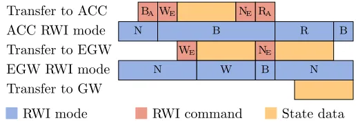
In the Figures that follow we will use letter to indicate the mode of the RWIs and the type of the commands that are sent. The modes are denoted with N, B, R and W which are normal, bypass, read and write respectively. The commands are denoted with the same letter and will change the mode accordingly. The commands have a subscript that indicates for which RWI the command is. An A is used to mark commands for the accelerator RWI and an E is used to mark commands for the exit gateway RWI.

Restore stage

the right place. This is done by sending a write commando to the exit gateway followed with some state data that contains the correct configuration. Finally all accelerators are put in normal mode by sending the normal command to each of them. Now the chain is ready to process data. Figure 3.6 shows all the described transfers and mode changes of this stage.

Transfer to ACC WA WE NA NE

ACC RWI mode B W B N

Transfer to EGW WE NE

EGW RWI mode B W B N

RWI mode RWI command State data Figure 3.6: Transfers and RWI modes during restore stage

Process stage

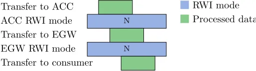
When the state of the accelerators is restored and the exit gateway is configured, the accelerator can be used to process data. Figure 3.7 shows that the entry gateway will send the data to the accelerator, it gets processed and the acceler-ator sends it to the exit gateway. The exit gateway knows who the consumer is and will send it the processed data.

When all the data send by the gateway, it can immediately start with the com-mands for the state-save. Because the accelerators will finish their calculation, before the RWI accepts the command, because the RWI waits for the done sig-nal from the accelerator. This means that the exit gateway no longer needs to signal the entry gateway that all data is processed and that it may perform a state-save.

Transfer to ACC

ACC RWI mode N

Transfer to EGW

EGW RWI mode N

Transfer to consumer

RWI mode Processed data

Figure 3.7: Transfers and RWI modes during process stage

Save stage

bypass by sending the bypass command. Next we send a write command to the exit gateway followed by the configuration data. We put the exit gateway in normal mode by sending the normal command. Now the exit gateway is configured and ready to receive state and send it to the entry gateway. So we send a read command to the accelerator, and the accelerator will start sending its state to the exit gateway. The exit gateway will then send the state to the entry gateway. The entry gateway will store the state and will use this in the next restore-save sequence.

Transfer to ACC BAWE NE RA

ACC RWI mode N B R B

Transfer to EGW WE NE

EGW RWI mode N W B N

Transfer to GW

Chapter 4

Dataflow Analysis

In this chapter we will describe the dataflow model of the previous architecture and we will propose a dataflow model for the proposed architecture. The first section in this chapter will introduce the dataflow model of the previous architec-ture. In the second section a new dataflow model is proposed that incorporates the changes in the proposed hardware architecture. The last section presents an abstraction of the proposed dataflow model. This chapter will require a basic knowledge of dataflow modelling.

Temporal analysis is an important part of real-time system design. It is used to give temporal guaranties over the design. Dataflow is one of the exiting analysis techniques. It is typically used to calculate worse case throughput, or to find optimal buffer sizes under throughput constraints. In [2] a new use of dataflow analysis is presented, the calculation of optimal packet sizes. The paper gives techniques to find optimal packet sizes under throughput constraints. The packet sizes dictate the granularity at which state-saves are performed. Small packet sizes result in high state-save overhead, while large packet sizes will increase latency and require bigger buffers. The ability to find optimum packet sizes is a nice addition to dataflow modelling, which will lead to better optimized designs.

4.1

Previous Accelerator Sharing Models

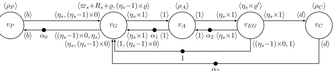
This model only has one accelerator, but multiple accelerators can be added in betweenvG andvEG.

First we explain what all the edges represent, and after this we explain the meaning of all symbols. The edge and the back edge betweenvP andvG

repre-sent the CFIFO buffer between the producing CPU and the entry gateway CPU. The variableα0 indicates the number of initial tokens on edge (vG,vP) which

corresponds with the capacity of the CFIFO betweenvP andvG. The edge and

back edge fromvGtovAand fromvAtovEGform the accelerator pipeline. The

edges represent the credit based communication between the components, that prevents the overflow of the local accelerator FIFOs. The edge from vEG to vG represents the synchronisation between the two that occurs when the entry

gateway waits until all the data is processed by the accelerator chain. The edge from vEG to vC shows that the CFIFO of the consumer is filled by the exit

gateway. However the back edge is fromvC to vG, because the entry gateway

has to reserve space in the CFIFO before the exit gateway can write to this CFIFO.

Symbolsb,ηsanddare packet sizes of the producer, gateway and consumer

re-spectively. The buffer size of the CFIFO between the producer and the gateway isα0, and between the gateway and the consumer is α3. The size of the

hard-ware buffers between the entry gateway and the accelerator isα1, and between

de accelerator and the exit gateway isα2. The firing durations of the producer,

accelerator and consumer areρP,ρA andρC respectively, which correspond to

the execution times of these components in the implementation. The variable%

represents the time that the gateway needs to send a sample to the accelerator. The variable%0 represents the time that the exit gateway needs to send a sam-ple to the consumer. Rsrepresents the time that the gateway needs in order to

reconfigure the accelerators. Lastly$srepresents the maximum delay that the

other streams introduce when the accelerator is shared.

vP vG vA vEG vC

hρPi h$s+Rs+%,(ηs−1)×%i hρAi hηs×%0i hρCi

hbi hηs,(ηs−1)×0i

α0 h(ηs−1)×0, ηsi

hbi

hηs×1i h1i

α1h1i

hηs×1i

h1i hηs×1i

α2hηs×1i

h1i

hηs×1i hdi

α3

hdi hηs,(ηs−1)×0i

1

h(ηs−1)×0,1i

h1,(ηs−1)×0i

Figure 4.1: Previous CSDF model

In [2] an abstraction of the CSDF model is made. The next paragraph will describe how this is done, later the same methods are used to make the abstrac-tion.

by creating an execution schedule for the gateways and the accelerator. This execution schedule is then used to bound the execution time ofvS.

vP vS vC

ρP γs ρC

b ηs

α0 ηs

b

ηs d

α3 d

ηs

1

Figure 4.2: Previous SDF model

The following equations are used in [2] to prove that the abstraction holds, Equation (4.1), Equation (4.2) and Equation (4.3). The multiple streams that managed by the gateway are denoted with the set S, where s is one of those streams. Whereτsis the time it takes to processηselements from stream son

the accelerators, including state-save overhead,Rs. The delay an other stream

can introduce due to sharing is$s. The total processing time of a stream isγs,

including the processing times from other streams that share the accelerator.

τs≤ˆτs=Rs+ (ηs+ 2)·max(%, ρA, %0) (4.1)

$s≤$ˆs= X

i∈S\s

ˆ

τi (4.2)

γs= ˆτs+ ˆ$s= X

i∈S

ˆ

τi (4.3)

Equation (4.1) shows thatτs is dependent on the state-save overhead (Rs) and

the packet size,ηs. The minimum processing time of one element in this pipeline

can be over-approximated by max(%, ρA, %0). The +2 comes from the fact that vG, vA, vEG, and the edges between them form a pipeline. So whenvG

pro-duces a token, it still needs to passvA and vEG resulting in a delay equal to

two additional firings. Equation (4.2) shows that when sharing an accelerator, the maximum time that a stream has to wait is the sum of all other streams. Finally Equation (4.3) concludes that the total processing time is the sum of all individual stream processing times.

4.2

Proposed CSDF model

changes made in the hardware. The two key differences between de previous and the proposed architecture are: state is transferred via the Nebula ring net-work and the entry gateway no longer checks if all the data is processed by the accelerators. The next paragraphs describe how these differences are included in the dataflow model.

Because the state and the data are now going over the same network it makes sense to model this as well. As the figures in Section 3.3.3 show, performing a state-save involves sending a complex sequence of data and commands to the accelerators and thus constantly changing the mode of the RWI.

Figure 4.3 shows the firing duration and, production and consumption quanta for all the different situations an accelerator and its RWI can be in.

vA ρN 1 1 1 1

(a) Data in normal mode

vA ρB 1 1 1 1

(b) Data in bypass mode

vA ρR 0 0 1 1

(c) Data in read mode

vA ρW 1 1 0 0

(d) Data in write mode

vA ρCO 1 1 0 0

(e) Command for this accelerator vA ρBC 1 1 1 1

(f) Command not for this accelerator

Figure 4.3: SDF models of the different accelerator behaviours

Note that the behaviour is dependent on the mode, which is changed with the commands. So it may look like we are trying to model data dependant behaviour in CSDF, which is impossible because a firing of an actor is only dependant on the arrival of tokens on its edges. However, because the exact sequence of commands and thus mode changes are known, it can be modelled as a CSDF. This is done by setting the firing duration and quanta vectors so that they mimic the behaviour of a state-save cycle. An example of this is given in Figure 4.4. It shows the first 10 situations the accelerator is in. These correspond with the actions described in Section 3.3.3.

vA

hρCO, ρW, ρW, ρW, ρBC, ρB, ρB, ρB, ρCO, ρBC, ...i h1,1,1,1,1,1,1,1,1,1, ...i

h1,1,1,1,1,1,1,1,1,1, ...i

h0,0,0,0,1,1,1,1,0,1, ...i

h0,0,0,0,1,1,1,1,0,1, ...i

Figure 4.4: CSDF model of an accelerators restore-save cycle

the entry gateway and exit gateway have changing behaviours. These are also deterministic and can be modelled with long firing duration and quanta vectors. Because the data and state are both send via the Nebula ring network, we assume that both will take% time. We assume the same for the exit gateway, sending data or state will both take%0 time.

The entry gateway no longer checks if all data is processed by the accelerators before it performs a state-save. Therefore the exit gateway no longer needs to signal the entry gateway. The signalling was represented by an edge fromvEG

tovG in the previous model, so that edge can be removed.

However because the state is now transferred via the ring network, an accelerator will send its state to the exit gateway. The exit gateway will send it to the entry gateway. Because the state is needed when the state is restored by the entry gateway, therefore the entry gateway is dependent on the exit gateway. So the entry gateway not only needs to check if there is data from the producer and reserve space in the buffer of the consumer, it also needs to check if the previous state is received. This is represented by an edge betweenvEGandvG, whereα4

represents the number of transfers needed in order to save the state.

The changes result in the proposed CSDF model, see Figure 4.5. It is a complex model due to the exact modelling of the restore-save cycle. While this will model the restore-save cycle correct, it does not model delays due to sharing the accelerator with other streams. In Section 4.3 we propose an additional model that is an abstraction of the CSDF model and does include the delays due to accelerator sharing.

vP vG vA vEG vC

hρPi h%, %, %, ...i hρCO, ρW, ρW, ...i hρCO, ρW, ρW, ...i hρCi hbi hηs,0,0, ...i

α0h0,0,0, ...i

hbi

h1,1,1, ..i h1,1,1, ...i

α1h1,1,1, ...i

h1,1,1, ...i

h0,0,0, ...i h1,1,1, ...i

α2h1,1,1, ...i

h0,0,0, ...i

h0,0,0, ..i hdi

α3

hdi hηs,0,0, ...i

α4

h0,0,0, ...i hα4,0,0, ...i

Figure 4.5: Proposed CSDF model

4.3

Proposed SDF model

In this section we will present an SDF model which is an abstract version of the CSDF model proposed in Section 4.2, which also includes the delay that is a result of the sharing of the accelerators. First we will create an SDF from the CSDF model by means of abstraction. Then we will add the delay that is the result of sharing of the accelerators.

In order to simplify the CSDF model, we will combine actorsvG,vA andvEG,

as well as the edges between these actors into one actor. We will also limit the number of phases to one, which results in a SDF model. In order to perform the abstraction, a schedule is created to visualize the firings. Figure 4.6 shows the schedule of the state-save sequence described in Section 3.3.3. As shown in Figure 4.6 the duration of a restore-save cycle depends on the number of transfers needed to restore the accelerator state, the number of data sample that are processed, the number of transfers needed to save the state and the number of commands. The total number of restore transfers isL, where li is

the number of transfers for a partial restore. The number of data samples that are processed is denoted withηs. This is also called the packet size. The total

number of save transfers will be called J, whereji is the number of transfers

for a partial save. The total number of commands isK. The firing durations in Figure 4.6 are all shown as equal, this is probably not true. However later we will over-approximate all the different firing durations into one uniform time step, and this will correspond with the uniform firing durations in Figure 4.6. This over-approximation is an valid abstraction, base on the the-earlier-the-better refinement. This refinement states that shorter firing duration can never result in a worse schedule.

vG % i1×% % i2×% % % ηs×% % % i3×% % %

vA ρCO i1×ρW ρBC i2×ρB ρCOρBC ηs×ρA ρCOρBC i3×ρB ρCOρBC j1×ρR

vEG ρCO i2×ρW ρCO ηs×%0 ρCO i3×ρW ρCO j1×%0

Figure 4.6: Typical schedule of the CSDF model

We can now derive an upper bound for the time it takes to perform a restore-save cycle. Equation (4.4) gives an upper bound on the duration of the restore-save cycle. The maximum possible firing duration of every actor is used to create an uniform time step. This time step is the worse case firing duration of every possible phase of actors vG, vA and vEG. With this uniform time step we can

create a schedule just like Figure 4.6. The number of uniform time steps needed to perform the restore-save sequence is equal to the number of transfers and the number of transfers is equal to the sum ofL,J,K andηs. Because production

by vG still needs to go through vA and vEG, two additional time steps are

necessary, which result in the +2 in Equation (4.4).

τs≤ˆτs= (L+J+K+ηs+ 2)·max(%, ρA, ρB, ρW, ρR, ρCO, ρBC, %0) (4.4)