http://www.scirp.org/journal/jamp ISSN Online: 2327-4379
ISSN Print: 2327-4352
DOI: 10.4236/jamp.2017.511186 Nov. 29, 2017 2291 Journal of Applied Mathematics and Physics
Application of Improved Artificial Bee Colony
Algorithm in Urban Vegetable Distribution
Route Optimization
Zhenzhen Zhang, Lianhua Wang
Beijing Wuzi University, Beijing, China
Abstract
According to the characteristics and requirements of urban vegetable logistics and distribution, the optimization model is established to achieve the mini-mum distribution cost of distribution center. The algorithm of artificial bee colony is improved, and the algorithm based on MATLAB software is de-signed to solve the model successfully. At the same time, combined with the actual case, the two algorithms are compared to verify the effectiveness of the improved artificial bee colony algorithm in the optimization of urban vegeta-ble distribution path.
Keywords
Urban Vegetable, Vehicle Routing, Optimized Artificial Bee Colony Algorithm, Path Optimization
1. Introduction
City vegetable logistics is engaged in transportation, warehousing and other se-ries of vegetable logistics activities within the city limits, it is one of the logistics, business flow and information flow, according to different customers on the de-livery time and quantity of vegetables and other requirements, to provide perso-nalized service for customers and distribution [1]. As the characteristics of the city itself, making the city vegetable logistics and distribution with a wide range of customers, the number of customer points, customer points between the dis-tribution distance is relatively close to the characteristics of urban vegetable lo-gistics and distribution generally use the car for distribution, not only because the special truck has the advantages of strong maneuverability, flexible response How to cite this paper: Zhang, Z.Z. and
Wang, L.H. (2017) Application of Im-proved Artificial Bee Colony Algorithm in Urban Vegetable Distribution Route Opti-mization. Journal of Applied Mathematics and Physics, 5, 2291-2301.
https://doi.org/10.4236/jamp.2017.511186
Received: October 19, 2017 Accepted: November 26, 2017 Published: November 29, 2017
Copyright © 2017 by authors and Scientific Research Publishing Inc. This work is licensed under the Creative Commons Attribution International License (CC BY 4.0).
http://creativecommons.org/licenses/by/4.0/
DOI: 10.4236/jamp.2017.511186 2292 Journal of Applied Mathematics and Physics
[2], and these advantages can also meet the customer a small number of goods, the number of purchases, delivery to the door of the consumer characteristics. In addition, the urban vegetable logistics and distribution of urban residents have a great impact on daily life. It is necessary to construct a reasonable urban vegeta-ble logistics and distribution system not only to meet the requirements of time-liness, convenience, distribution environment and high distribution efficiency, but also should meet the characteristics of urban customers, distribution flow and other characteristics [3].
Urban vegetable logistics distribution vehicle routing problem can be scribed as: there are a number of customers need the distribution center to de-liver a certain amount of goods, the specific location of each customer point is known. The distribution center with the delivery task has the same type of dis-tribution vehicle, and the quantity meets the demand, all the delivery vehicles have the same carrying capacity of [4]. The vehicles that carry the goods depart from the distribution center, along the planned route, the goods to the customer on the route of the hands of the final return to the distribution center. There are certain conditions in the distribution process constraints, each customer can only be a distribution vehicle responsible for the distribution of the task, the time of delivery of the goods within the time required by the customer, other-wise given the appropriate delivery vehicle must be punished [5] [6]. In this pa-per, the establishment of the model first considers the requirements of the cus-tomer point to the delivery time, and then considers the optimization model with the total cost as the goal, which is based on the load and distance con-straints of the vehicle. Using the improved artificial bee colony algorithm, using MATLAB software programming solution, combined with the case, to verify the feasibility and effectiveness of improving the artificial bee colony algorithm.
2. Establishment of Model
2.1. Assumptions
As a result of the actual distribution, we will encounter a variety of practical problems, from a different point of view, to solve the problem achieved by the target results are not the same, in order to study and establish the issue of urban vegetable distribution mathematical model [7]. Here make the following as-sumptions: 1) The starting point of each delivery vehicle for the distribution center, and ultimately return to the distribution center. 2) The total delivery amount of each distribution route is less than the maximum load of the vehicle. 3) The distance traveled by each delivery vehicle shall not exceed its distance. 4) Each customer can only be completed by a car distribution, the cost of each ve-hicle start and travel unit distance is known.
2.2. Model Establishment
DOI: 10.4236/jamp.2017.511186 2293 Journal of Applied Mathematics and Physics (a) S=
{
i i| =0,1, 2,,n}
: collection of a single distribution center and all of its customers, i=0 is the distribution center, i=1, 2,,n is customer whoprovides delivery services by the distribution center;
(b) K=
{
k k| =0,1, 2,,m}
: a set of vehicles that can be used by thedistribu-tion center;
(c) Q: the maximum load of a vehicle, in which the vehicle is the same type of vehicle;
(d) qi: the customer needs, that is, distribution center should be provided for
the customer point of delivery, i=1, 2,,n;
(e) D: the maximum distance of the vehicle is the same type of vehicle, so the maximum distance is the same;
(f) dij: the distance from the point i to the point j, i j, =0,1, 2,,n;
(g) tij: the time is used from point i to point j, i j, =0,1, 2,,n;
(h) C0 is the fixed cost of the vehicle, the starting cost required for each ve-hicle to be delivered, C1 is the distance traveled by the vehicle, the cost per unit length of time per vehicle;
(m) ti: the time at which the vehicle serves the customer, i=0,1, 2,,n;
(p) Sik: the time period during which the vehicle provides services to the
customer, Sike and Sikl are the starting and ending time of vehicles serving
customers respectively, i=0,1, 2,,n;
(r) ET LTi, i: the customer service time window start and end time, during
this time to provide delivery services is the highest customer satisfaction, 0,1, 2, ,
i= n;
(v) P Si
( )
ik : the penalty cost caused by the service of the customer, that is, thepunitive cost caused by the failure to provide service at the time of customer sa-tisfaction.
(w) xijk: whether or not the vehicle provides service from the customer to the
customer, i j, =0,1, 2,,n, k=1, 2,,m;
(q) yik : whether the vehicle provides the customer with the delivery,
1, 2, ,
i= n, k=1, 2,,m,
The decision variables for the problem are as follows: 1 the vehicle is served from point to point
, 0,1, 2, , ; 1, 2, ,
0 otherwise
ijk
i j
x = i j= n k= m
1 the task of customer is done by vehicle
1, 2, , ; 1, 2, ,
0 otherwise
ik
i k
y = i= n k= m
In this question, the penalty coefficient is introduced and the opportunity cost is expressed as the unit weight per unit time. When the distribution vehicle fails to provide service in the customer satisfaction period, it will be punished in cer-tain proportion. When the actual delivery time is earlier than the service time window, the penalty coefficient is α, when the actual delivery time is later than the service time window, the penalty coefficient is β. P Si
( )
ik formula of penaltyDOI: 10.4236/jamp.2017.511186 2294 Journal of Applied Mathematics and Physics
( )
(
)
(
)
0 , 0,1, 2, ,
i i ike ike i
i ik i ike ikl i
i ikl i ikl i
q ET S S ET
P S ET S S LT i n
q S LT S LT
α
β
− <
= ≤ ≤ =
− >
(2-1)
When the cost of cargo damage is calculated, it is assumed that the damage rate of the vegetables is related to the time of the vegetables in the prescribed low-temperature transportation environment, and the deterioration rate of the vegetables is constant and the deterioration rate of the vegetables is constant and the metamorphic function [8] as follows:
e t
i i
Q′ =Q C −δ (2-2)
Among them, Qi the product is the quality of the goods in good condition,
t is the product experience the logistics time, δ is the product of the sensitiv-ity coefficient of time, C for the product at a constant temperature
deteriora-tion of a constant speed change. In the metamorphic funcdeteriora-tion, the product is more sensitive to time, the δ value is relatively small, on the contrary, the
val-ue is larger.
The cost of the entire distribution process is:
(
)
1
1 e ike n
S i
i
H q C −δ p
=
=
∑
− (2-3)p is the unit of the value of the loss of vegetable products.
The VRPSTW studied in this paper will be time cost, with the lowest total cost as the optimization target. The objective function is shown in (2-4).
( )
(
)
1 0 0
1 0 0 1 0 1 1
min 1 e ike
m n n n n m n
S ij ijk i ik i k i
k i j i i k i
Z C d x P S C x q C −δ p
= = = = = = =
=
∑∑∑
+∑
+∑∑
+∑
− (2-4)The constraints are:
1
, 1, 2, ,
n i ik i
q y Q k m
=
≤ =
∑
(2-5)1
1, 1, 2, ,
m ik k
y i n
=
= =
∑
(2-6)0 1 m k k y m = =
∑
(2-7)0 1
1, 1, 2, ,
n jk j
x k m
=
= =
∑
(2-8)0 1
1, 1, 2, ,
n i k i
x k m
=
= =
∑
(2-9)0
, 1, 2, , ; 1, 2, ,
n
ijk jk i
x y j n k m
=
= = =
∑
(2-10)0
, 0,1, , ; 1, 2, ,
n
ijk ik j
x y i n k m
=
= = =
∑
(2-11)0 0
, 1, 2, ,
n n ij ijk i j
d x D k m
= =
≤ =
DOI: 10.4236/jamp.2017.511186 2295 Journal of Applied Mathematics and Physics 0,1, , 0,1, , ; 1, 2, ,
ijk
x = i j= n k= m (2-13)
0,1, 0,1, , ; 1, 2, ,
ik
y = i= n k= m (2-14)
(
1)
,0,1, , ; 0,1, , ; 1, 2, ,
ike i ijk ij ijk ijk jke
S t x t x M x S
i n j n k m
+ + − − ≤
= = = (2-15)
(
1)
, 0,1, , ; 0,1, , ; 1, 2, ,ikl ij ijk ijk jke
S +t x −M −x ≤S i= n j= n k= m (2-16)
, 0,1, , ; 1, 2, ,
ikl ike i ik
S =S +t y i= n k= m (2-17)
, 0,1, , ; 1, 2, ,
ike ik
S ≤My i= n k= m (2-18)
0, , 0,1, , ; 1, 2, ,
ike ikl ike
S ≥ S ≥S i= n k= m (2-19)
0ke 0, 0kl 0, 1, 2, ,
S = S = k= m (2-20) The description of the constraint is as follows: Equation (2-5) indicates that the total demand for all customers per vehicle service does not exceed the capac-ity limit of the vehicle. (2-6) (2-8) means that each customer point can only be delivered by one car. Type (2-7) means that each vehicle from the distribution center. (2-9) means that each car finally returns to the distribution center. (2-10) means that each car if the arrival point must be service. (2-11) means that if the vehicle is customer service, the vehicle will leave the point after the task is com-pleted. Equation (2-12) indicates that the total travel distance of each vehicle must not exceed its travel distance limit. (2-15) and (2-16) show the time rela-tionship in which the vehicle arrives at two customers in their distribution route. Equation (2-17) indicates the relationship between the starting and ending time of the vehicle for customer service. (2-18) means that if the vehicle does not pro-vide delivery to the customer, the vehicle will not reach the customer. Equation (2-19) represents the time limit for the start and end of the service time for the customer service. Equation (2-20) indicates that the departure time of the vehicle from the distribution center is zero.
3. Improved Artificial Bee Colony Algorithm
Human beings based on the nature of bees to collect honey activities, summed up the artificial anthropocentric algorithm theory and to describe. The take bee (the lead bee) to go out looking for honey, and then by jumping dancing and another worker bees in the form of probability to share the source of food in-formation, follow the bee and reconnaissance bee first wait, until the bees bring back the food source information, then choose to follow the honey or find the food near the source to find nectar. From the above description can be learned to adopt bees, follow the bee and reconnaissance bee be able to achieve the iden-tity of the conversion.
3.1. Parameter Initialization
DOI: 10.4236/jamp.2017.511186 2296 Journal of Applied Mathematics and Physics in each distribution vehicle. In the actual urban vegetable distribution vehicle routing problem, qi represents customer demand. The expression formula for setting N before the initialization phase is as follows:
1 1 n i i q N m q = = − +
∑
(3-1)Population size N = 50; N/2 indicates the number of food sources is also the number of honey mining bee; single maximum limit = 20; maximum number of iterations MaxCycle = 500.
Solution of the initialization function [solu] = Initial (num), this method is used to generate the problem of the initial solution. Method of production: by looking for the nearest customer service point, one by one distribution, and meet the constraints.
The solution space is defined by V[N][n][n], and the initial feasible solution number is denoted by N.
[ ][ ][ ]
0 1, ,v i j = − i∈N j∈n (3-2)
3.2. Evaluation Method of Profitability
Based on the optimization model of the urban vegetable distribution VRP prob-lem created by the objective function Formula (2-4), we can see that the actual problem to achieve is to minimize the total distribution costs. Artificial colony algorithm uses the reciprocal of the minimum distribution cost as the fitness function, so that the high cost corresponds to the low fitness and the small food source income value.
3.3. Population Update
The algorithm at the beginning of operation, there is not much difference in the probability of each food source is worker to find the number of iterations, a gradual increase in worker, not only to expand the search probability of each food source, and previously set good pheromone is gradually cut, resulting in not being left in to find a food source on early in the process of iterative phero-mone is nearly equal to zero. In addition, in the posterior iteration of the algo-rithm, the algorithm will generate local extreme value because of the large amount of information gathered on the path. The update formula is as follows:
(
)
( )( )( )
( )
( )
( )
1 max 1 min , 1 , N ij ij ij N ij ijQ N Q N Q Q Q N
Q N Q N Q Q
ε ε
ρ
ρ
+ − + ∆ + = + ∆ (3-3) Formula: ε
( )
N =N τ, τ is a constant. According to this formula can beachieved with the change of the pheromone solution to adjust the use of such methods can improve the efficiency of the ABC algorithm in the global scope, and can effectively prevent the local extreme situation.
set-DOI: 10.4236/jamp.2017.511186 2297 Journal of Applied Mathematics and Physics ting of the constant is as shown in Equation (3-4).
1 1
2 1 2
3 2 max
, 0
,
,
N N
N N N
N N NC
δ
δ δ
δ
≤ <
= ≤ <
≤ <
(3-4)
3.4. Nectar Selection
Follow the bee according to the nectar fitness value corresponding to the se-lected probability to choose the appropriate honey to go honey, the formula is as follows:
1
i
i N
i i
fit P
fit
= =
∑
(3-5)Follow the bee according to the nectar fitness value corresponding to the se-lected probability to choose the appropriate honey to go honey, the formula such as follow the bee to a certain probability in the poor near the nectar to find a new source. Compare the current nectar and the previous nectar fitness value, if the former is greater than or equal to the latter, then use the current nectar to re-place the previous nectar, otherwise, remain unchanged.
3.5. Population Elimination
When the bees (or follow bees) continuous limit failed to search better circula-tion nectar, this solucircula-tion is determined (i.e. the nectar will fall into the local op-timal solution). Bees (or follow bees) to give up the nectar, and into the investi-gation bee, continue to search for new nectar, the search formula is:
[ ]
(
)
min 0,1 max min
ij j j j
x =x +rand x −x (3-6)
4. Case Analysis
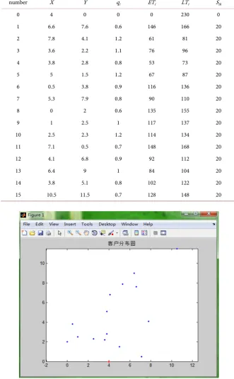
The distribution center of an enterprise provides distribution service for 15 cus-tomer points. The distribution center is represented by the serial number 0, and the serial number 1 - 15 represents 15 clients respectively. The enterprise uses the same type of freight car for 15 customer point distribution. Among them, the maximum carrying capacity of each car is 5 tons, the vehicle fixed cost is 100, the consumption time cost of 250 vehicles, earlier than the time window to the cus-tomer point penalty cost is 250 per ton per hour, the vehicle later arrived time windows penalty cost customers per ton of 300 per hour. The distribution center and customer information statistics are shown in Table 1. It is necessary to ar-range vehicles to complete the distribution task, so that the total cost of the tribution cost and the penalty cost is the least, so as to find the reasonable dis-tribution route for the disdis-tribution center. Data processing was carried out by Matlab2010 software.
DOI: 10.4236/jamp.2017.511186 2298 Journal of Applied Mathematics and Physics
Table 1. Distribution center and customer information.
number X Y qi ETi LTi Sik
0 4 0 0 0 230 0
1 6.6 7.6 0.6 146 166 20
2 7.8 4.1 1.2 61 81 20
3 3.6 2.2 1.1 76 96 20
4 3.8 2.8 0.8 53 73 20
5 5 1.5 1.2 67 87 20
6 0.5 3.8 0.9 116 136 20
7 5.3 7.9 0.8 90 110 20
8 0 2 0.6 135 155 20
9 1 2.5 1 117 137 20
10 2.5 2.3 1.2 114 134 20
11 7.1 0.5 0.7 148 168 20
12 4.1 6.8 0.9 92 112 20
13 6.4 9 1 84 104 20
14 3.8 5.1 0.8 102 122 20
15 10.5 11.5 0.7 128 148 20
Figure 1. Distribution center and customer distribution.
4.1. Case Solving and Analysis
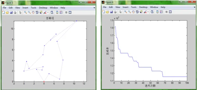
[image:8.595.205.537.95.631.2]DOI: 10.4236/jamp.2017.511186 2299 Journal of Applied Mathematics and Physics middle 51 - 150 times, Delta 2 = 50, 50 times after the iteration, Delta 3 = 200. The distribution route diagram and convergence process of artificial bee colony algorithm are shown in Figure 2, and the distribution route diagram and con-vergence process of artificial bee colony algorithm are improved, as shown in
Figure 3.
4.2. Comparison of Different Algorithms
In order to facilitate the comparison, the paper analyzes the data of the same en-terprise and the customer point of the same group. On the basis of the same dis-tance, traffic volume and distance limit, the optimization process of vehicle routing problem under soft time window constraint is simulated, The optimal target value of the algorithm is the total cost of distribution, and the specific data of the number of iterations of the total distribution vehicle convergence are shown in Table 2.
[image:9.595.206.539.370.523.2] [image:9.595.208.536.555.700.2]Comparison of the case data can be seen, the same customer restrictions on the distance, distance, volume, when the time constraint is not too strict, is the vehicle routing problem with soft time windows, an improved artificial bee co-lony algorithm in general distribution vehicle problems and artificial bee coco-lony algorithm is the same, but the distribution of the total cost savings of 1091.78;
Figure 2. Distribution route and convergence process for algorithm.
DOI: 10.4236/jamp.2017.511186 2300 Journal of Applied Mathematics and Physics
Table 2. Result comparison.
case cost vehicle Iteration times
1 11547.11 1 68
2 10455.33 1 50
and convergence the speed of the improved artificial bee colony algorithm is faster. The main reason is the analysis algorithm, improved artificial bee colony algorithm with variable neighborhood search update strategy, the best individual search direction is better than stronger, compared with the traditional artificial bee colony algorithm, optimize the operation speed and quality optimization.
5. Conclusion
Logistics and distribution activities is an important part of the logistics system to achieve the optimization of vehicle routing that can directly optimize the logis-tics and distribution activities, not only can improve the economic efficiency of enterprises, but also to help achieve the logistics management of scientific. Ve-hicle routing problem as a combinatorial optimization problem, has a strong theory, application value, in the field of logistics and distribution has been wide-ly used [9]. Although the degree of attention to the research of vehicle routing problem is growing, but the expansion of the basic distribution routing problem with time constraint is not deep enough, but has yet to find the solution more quickly and accurately, so there are many scholars pay close attention in the li-mited time to find the most satisfactory solution to the problem of [10]. On the basis of the previous scholars’ research, this paper studies the vehicle routing problem with time constraints, takes into account the influence of time on the distribution path, analyzes the different criteria of the customer’s time require-ments, but the problems studied in this paper do not consider the actual distri-bution. The impact of road conditions on the speed of the road, in the next step can also be added to the peak period, the impact of non-peak time on the speed of the introduction of real-time changes in speed to study.
References
[1] Huang, H. and Zhang, Z.X. (2010) Research Status and Prospect of Vehicle Routing
Problem. Logisticstechnology, 10, 21-24.
[2] Nourossana, S. and Erfani, H. (2012) Bee Colony System: Preciseness and Speed in
Discrete Optimization. International Journal on Artificial Intelligence Tools, 21,
1250006-1250016.https://doi.org/10.1142/S0218213011000474
[3] Lan, H. and He, Q.F. (2015) Optimization of Cold Chain Logistics Distribution
Route Considering Road Access. Journal of Dalian Maritime University, 41, 67-74.
[4] Bi, X.J. (2012) Improved Artificial Bee Colony Algorithm. Journal of Harbin
Engi-neering University, 33, 117-123.
[5] Bao, W.W. and Liu, T. (2012) A Survey of Artificial Bee Colony Algorithm. Shanxi
DOI: 10.4236/jamp.2017.511186 2301 Journal of Applied Mathematics and Physics
[6] Ozturk, C., Hancer, E. and Karaboga, D. (2015) Dynamic Clustering with Improved
Binary Artificial Bee Colony Algorithm. Applied Soft Computing, 28, 69-80.
https://doi.org/10.1016/j.asoc.2014.11.040
[7] Shao, K. Research and Application of Vehicle Routing Problem Based on Artificial
Bee Colony Algorithm. Master Thesis, Wuhan University of Technology, Wuhan.
[8] Wang, Q. Study on Logistics Distribution Location and Transportation Route
Op-timization of Cold Chain Food with Time Window. Master Thesis, Changan Uni-versity, Xi’an.
[9] Yang, J. and Ma, L. (2010) Application of Bee Colony Optimization Algorithm in
Vehicle Routing Problem. Computer Engineering and Applications, 46, 214-216.
[10] Yu, X.D. and Lian, L. (2016) Application of Artificial Bee Colony Algorithm in
Ve-hicle Routing Problem with Single Time Windows. Science and Technology