Munich Personal RePEc Archive
A Theory of Dichotomous Valuation with
Applications to Variable Selection
Hu, Xingwei
International Monetary Fund
15 June 2017
Online at
https://mpra.ub.uni-muenchen.de/80457/
A Theory of Dichotomous Valuation with Applications
to Variable Selection
Xingwei Hu1
International Monetary Fund, 700 19th St NW, Washington, DC 20431, USA
Abstract
An econometric or statistical model may undergo a marginal gain when a new
variable is admitted, and marginal loss if an existing variable is removed. The
value of a variable to the model is quantified by its expected marginal gain and
marginal loss. Under a prior belief that all candidate variables should be treated
fairly, we derive a few formulas which evaluate the overall performance of each
variable. One formula is identical to that for the Shapley value. However, it
is not symmetric with respect to marginal gain and marginal loss; moreover,
the Shapley value favors the latter. Thus we propose a unbiased solution. Two
empirical studies are included: the first being a multi-criteria model selection
for a dynamic panel regression; the second being an analysis of effect on hourly
wage given by additional years of schooling.
Keywords: unbiased multivariate Shapley value,variable selection,
marginal effect,endowment bias,model uncertainty
JEL Classification Number: C11, C52, C57, C71, D81
1. Introduction
The problem with which we are concerned relates to the following typical
situation: When modeling data, we attempt to use a formula to simplify the
Email address: [email protected](Xingwei Hu)
1
underlying process that has been operating to produce the data. To be useful,
the model should not only help us to better understand the underlying structure
5
of the variables in the past, but also be predictive in a non-specific situation in
the future; ideally, it should perform well under multiple criteria. In general, the
variables may either correlate with or be interdependent on each other. Some
variables may even be explained by other variables; thus, they are highly
super-fluous. Others may simply be irrelevant to the underlying process. Selection of
10
right variables in modeling and forecasting the underlying process is one of the
most fundamental problems in statistics and econometrics.
In this paper, we incorporate rather than ignore model uncertainty and
derive a few formulas to be used in variable selection, by evaluating the
contri-bution of each variable in a large set of modeling scenarios . The exposition is
15
self-contained and the approach employed is game-theoretic and Bayesian. For
a simple context, letY denote the dependent variables in the model, and let the
universal of candidate explanatory variables be indexed by N ={1,2,· · ·, n}.
We use “i” for the singleton set {i} and “\” for set subtraction. For any set
T ⊆N, let |T|denote the cardinality of T, and letv(T) be a vector of
collec-20
tive performance measures when we model the dataY using all variables inT.
In particular, for the empty set ∅, v(∅) is the performance measures when the
model does not involve any variables inN; say, for example, when modelingY
by a constant or a linear trend. The performance measures could be a measure
of model fit, variance explained, predictive power, negative of the cost function,
25
probability of avoiding fatal errors, or any combination of the above.
For a given performance function v: 2N →Rm, our goal is to find a small
set of variables that have high importance with respect to v. Unlike many
algorithm-based approaches, which search for a subset of variables with optimal
collective performance, we directly evaluate the overall performance of each
30
variable under a fair prior belief. Then, we use their performance to select
variables and institute the model. The search for a single model, however,
ignores the model uncertainty. By the term “overall performance,” we mean
model. Thus, a prior belief or distribution is required to specify the possibility
35
of modeling scenarios; in this sense, our approach is also Bayesian and uses
model averaging (e.g., George and McCulloch, 1997; Clyde and George, 2004;
O’Hara and Sillanpaa, 2009). Given special classes of priors, we show that the
expected performance coincides with the Shapley value and the Banzhaf value
in the coalitional game (N, v). We also suggest a new value concept which
40
embraces both the Shapley value and the Banzhaf value.
The results in this paper arise from considering any marginal effect to be
either a marginal loss or a marginal gain. As an example, consider the
con-tribution of a bachelor’s degree (hereinafter “BD”) to the annual income of an
individual aged 40. The individual may have a BD or not. For an individual
45
with a BD, a marginal gain is computed as the difference between his current
annual income and his estimated annual income, assuming he had no BD,
ce-teris paribus. On the other hand, a marginal loss for an individual with no
BD is computed as the difference between his current annual income and his
estimated annual income, assuming he had a BD,ceteris paribus. We note that
50
the possession of a BD is interwoven with other factors, such as his profession
and length of relevant work experience, which also affect his income. We define
the value of a BD as the expected marginal gain and marginal loss,
incorporat-ing the ownership uncertainty and the interdependence with other factors. In
addition, a BD holder may show some endowment bias, valuing the BD more
55
than those who don’t have a BD; we define the bias as the expected difference
between the marginal gain and loss.
Our research here is closely related with the Shapley value (Shapley, 1953).
Recently, the use of the Shapley value in modeling data has gained popularity
(e.g., Lipovetsky and Conklin, 2001; Israeli, 2007; Gromping, 2007; Devicienti,
60
2010; Budina et al., 2015), partly owing to its simplicity and generality. The
vast literature also provides us with many variations on the Shapley value (cf
Donderer and Samet, 2002; Winter, 2002). Our research here provides not only
a new proof and a new interpretation of the Shapley value, but also a theoretical
foundation for properly using the value concept in variable selection and related
fields. Theorem 1 in this paper was previously proved in Hu(2002); the first
two theorems of this paper are a generalization of the results in Hu (2006) in
which the grand cooperation is not necessary and v(T) is a binary function
representing a vote passing or blocking by the voters ofT.
The advantage of our approach is fivefold. First, the performance
measure-70
ment v is a vector function and thus extends the Shapley value to the
mul-tivariate case. As a consequence, the variable selection eventually becomes a
multi-criteria decision analysis, mitigating the discrepancy between model
ac-curacy and usefulness. Secondly, we acknowledge the model uncertainty and
the inter-linking among the variables; we address them using a prior
distribu-75
tion or prior belief. Any further specifications or restrictions can also be added
to the priors. Thirdly, by dichotomizing the marginal effect, we generalize the
Shapley value and the Banzhaf value under a same framework; they differ in
prior uniform distributions. Next, we discover the symmetry in the Banzhaf
value and asymmetry in the Shapley value and suggest a simple adjustment to
80
be used in the applications. Lastly, under the same framework we introduce
a new valuation solution based on binomial distributions. It is as tractable in
expression and calculation as the Shapley value and the Banzhaf value;
addi-tionally, it allows the expected model size from the prior to be consistent with
the model being estimated. Moreover, it has a constant endowment bias ratio
85
and relates to all other value concepts discussed in this paper.
The paper is organized as follows. Section 2 formulates the essential ideas
of dichotomized marginal effect and relate them to the Shapley value and the
Banzhaf value. Next, sections 3 analyzes the difference, calledendowment bias,
between the expectations of marginal gain and marginal loss. In this section,
90
a weighted unbiased value concept is proposed. After that, section 4 discusses
how to implement the basic ideas by a sequential algorithm. In section 5, we
conduct two empirical studies. In section 6, we relate this framework to several
other topics in economics, finance, and statistics. Proofs and large tables are
contained in the Appendix.
2. Evaluation of Candidate Predictors
To address the model uncertainty, let the random set S ⊆ N be the set
of variables in the model. The randomness of S arises from both objective
uncertainty and subjective one. For the objective uncertainty, an econometric or
statistical model is merely an approximation and simplification of reality−Box
100
(1976) even claimed that all models are wrong−and there could be many good
approximations under various criteria. For the subjective uncertainty, we do not
know exactly which specific variables to choose before performing a selection
analysis; we may have a class of subjective probabilities for it, derived from our
personal judgment, opinions, past experience, or even fairness assumptions.
105
Let µ be the distribution of S with PT being the probability of S = T.
Without any specific prior knowledge, we have no reason to believe that one
set of candidate variables is more likely to be Sthan another set of the same
size. That is, we should not discriminate between sets of variables having the
same size. To put it in another way, given the size ofS, we have no reason to
110
select one variable and reject another. This argument is formally justified by
theprinciple of insufficient reason and defines a class of distributions:
Fdef= {µ|PT is a function depending only on the size ofT}.
For the indeterminateS, we could add one variable fromN\Sto the model
or we could remove an existing variable from the model. The worth of the
115
addition or removal can be explained by the variable’smarginal effect tov(S).
• Scenario 1: i∈S. Then, i’s marginal effect isv(S)−v(S\i), called
marginal gain, in that it contributesv(S)−v(S\i) when we include it
into the model. The expected marginal gain, due toi’s participation
inS, is
γi[v;µ]def= Ev(S)−v(S\i).
• Scenario 2: i6∈S. Then, the marginal effect isv(S∪i)−v(S) in that
Sfaces a marginal loss or opportunity cost v(S∪i)−v(S) without
variable iin the model. In other words, the ith variable could have
increased the collective performance byv(S∪i)−v(S) if we had added
it toS. The expected marginal loss, due toi’s absence fromS, is then
λi[v;µ]def= E
v(S∪i)−v(S)
.
In either case, the marginal effect ofitov(S) can be written asv(S∪i)−v(S\i).
Combining these marginals, we define variable i’s dichotomous value ψi[v;µ]
120
(hereinafter, “D-value”), as a functional function ofv, by its expected marginal
effect under the distributionµ:
ψi[v;µ]def= γi[v;µ] +λi[v;µ]. (1)
Equivalently,
ψi[v;µ]def= Ev(S∪i)−v(S\i). (2)
In other words, the D-value ψi[v;µ] quantifies variablei’s overall performance
in v under the distribution µ, which itself specifies the likelihood of modeling
125
scenarios. Formally, one could derive (2) from two axioms:
• Marginality: givenPT = 1, ψi[v;µ] =v(T∪i)−v(T\i);
• Linearity: for anyµ1,µ2on 2N and any 0≤α≤1,
ψ[v;αµ1+ (1−α)µ2] =αψ[v;µ1] + (1−α)ψ[v;µ2].
Besides, one of our objectives is to apply the D-value ψ[v;µ] to distribute
requires thatµsatisfies the functional equation of
130
n
X
i=1
ψi[v;µ] =v(N)−v(∅). (3)
Thus, the portionψi[v;µ] ofv(N)−v(∅) is explained by variablei. The following
theorem relates the D-valueψ[v;µ] with the Shapley value Ψ[v] in the coalitional
game (N, v), defined as:
Ψi[v]
def
= X
T⊆N
(|T| −1)!(n− |T|)! n!
v(T)−v(T\i)
.
Theorem 1. For any µ∈ F which satisfies (3), we haveψ[v;µ] = Ψ[v]and
PT =
(|T|)!(n− |T|)! (n+ 1)! + (−1)
|T|η (4)
for anyη which guarantees the non-negativity of all PT’s.
Corollary 1. If PT is as in (4), thenµ∈ F andψ[v;µ] = Ψ[v].
In deriving the proofs, we assume neither v(∅) = 0, nor monotonicity ofv,
nor superadditivity ofv(i.e.,v(X∪Y)≥v(X) +v(Y) for any disjointX andY
135
inN). As shown by (4),µis not even unique. Besides, in the benchmark prior
withη= 0,|S|has the uniform distribution on the integers 0,1,· · ·, n.
In the game theory literature, there is another value concept called the
Banzhzf valueb[v] (Banzhaf, 1965) which is defined as
bi[v]
def
= 1
2n−1
X
T
v(T)−v(T\i)
.
In the next theorem, we associate the Banzhaf value with the D-valueψ[v;µ]
through another benchmark distribution, the uniform distribution on 2N.
Theorem 2. ψ[v;µ] =b[v]if and only if PT =
1
2n + (−1)|T|η for some η with
140
|η| ≤ 1 2n.
In this benchmark distribution (withη = 0), the model size|S|has a binomial
distribution with parametersn and.5. Note that in both benchmark
distribu-tions, the model Shas an expected size n
especially when applied in big data analytics. To solve the puzzle, we may use
145
priors with nonzeroη in which the density function PT oscillates with the size
|T|; we could also consider other distributions for|S|.
Theorem 3. If µ∈ F and|S|has a distribution of Binomial(n, p), then
PT =p
|T|(1−p)n−|T|
and
ψi[v;µ] = 1pγi[v;µ] = 1−1pλi[v;µ]
= P
T
p|T|−1(1−p)n−|T|
v(T)−v(T\i)
. (5)
In the binomial distribution, the modelShas an expected size ofnp.
3. Endowment Bias
150
In our valuation paradigm, we classify two types of marginal effect according
to the ownership: i ∈ S or i 6∈ S. In practice, people tend to value more on
things they own, rather than ones they do not own − even when things are
exchangeable in value. This subjective bias is called theendowment effect or
endowment bias. In this section, we first define the bias and then analyze the
155
implied bias in the Shapley value and the Banzhf value.
For i, we define itsendowment bias as the difference between its expected
marginal gain and its expected marginal loss,
κi[v;µ]def= γi[v;µ]−λi[v;µ].
Lemma 1 provides a method to calculate biases directly without involving the
expected marginal gain or loss.
Lemma 1. κi[v;µ] =P T
h
2PT −PT∪i−PT\i
i
v(T).
In Lemma 1, the weights ofv(T)’s sum to zero; but the bias itself may be not.
160
The following two theorems indicate strong association between the endowment
Theorem 4. The endowment bias κ[v;µ] = 0 if and only if µ is the uniform
distribution on2N, the benchmark distribution for the Banzhaf value.
Theorem 5. Given µ∈ F, the total biasP
i
κi[v;µ] = 0if and only if µ is the
165
uniform distribution on2N.
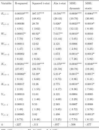
The Shapley value, however, tends to demonstrate strong evidence of
nega-tive endowment bias, largely due to the diminishing marginal effect ofv. This
counterintuitive issue could bring the users undesirable inference from the data
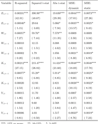
and eventually limits the usage of the value. Whenv is a set of modeling
crite-170
ria, in general, the candidate variables are modestly correlated with each other;
as a consequence, for anyi 6∈ T, its explanatory and predictive power is
par-tially mitigated by the members ofT. Moreover, the larger the setT, the likely
more the mitigation; thus, superaddtivity assumption is highly artificial, and
diminishing marginality is more pervasive.
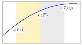
[image:10.612.239.370.380.453.2]175
Figure 1: Diminishing Marginal Effect for a Typical SetT
Let us formally define the diminishing marginality. Ideally, we expect the
inequality
v(T)−v(T \i)≥v(T∪j)−v(T)
holds for a typical T, i ∈ T and j 6∈ T as in Figure 1. But it is laborious to
locate the typicalT and it is impractical for the inequality to hold for all T’s.
Thus, we average both sides of the inequality for allT’s of sizet, alli∈T and
allj 6∈T. Obviously, the averages are
ωt
def
= (t−1)!(n!n−t)! P
|T|=t
P
i∈T
[v(T)−v(T\i)], t= 1,2,· · ·, n;
πt
def
= t!(n−nt!−1)! P
|T|=t
P
j6∈T
We sayv hasdiminishing marginal effect ifωt ≥πt fort= 1,2,· · ·, n−1; we
also say v has diminishing marginal gain (or diminishing marginal loss) if ωt
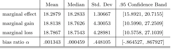
(orπt, respectively) is a decreasing function oft.
Theorem 6. πt = ωt+1 for t = 0,1,· · ·, n−1. Consequently, the following
statements are equivalent: 1. v has diminishing marginal effect; 2. v has di-180
minishing marginal gain; 3. v has diminishing marginal loss.
Theorem 7. Assume PT =
(|T|)!(n−|T|)!
(n+1)! , the benchmark prior for the Shapley
value. If v has diminishing marginal effect, then Pn
i=1
κi[v;µ]≤0; if v is
super-additive, then
n
P
i=1
κi[v;µ]≥0.
In an objective valuation, such as variable selection, either positive or
neg-185
ative endowment bias should be avoided. In (1), we place the same weight on
the marginal loss as on the marginal gain. To mitigate the endowment bias, one
could study theunbiased D-value defined as
˜
ψi[v;µ]def= (1−α)γi[v;µ] + (1 +α)λi[v;µ]. (6)
whereα=
P
j κj[v;µ]
P
j
ψj[v;µ], calledendowment bias ratio, is the ratio between the total
endowment bias and the total D-value. Clearly, there is no more endowment
bias in the unbiased D-value:
P
i
(1−α)γi[v;µ]−P i
(1 +α)λi[v;µ]
= P
i
(γi[v;µ]−λi[v;µ])−αP i
[image:11.612.113.480.163.675.2](γi[v;µ] +λi[v;µ]) = 0.
Figure 2: The Endowment Bias Ratio
In general, the endowment bias ratio α lies between −1 and 1 when v is
190
α is significantly positive, then P
j
γj[v;µ] > P j
λj[v;µ] and we have positive
endowment bias; we should place more weights on the expected marginal loss.
In contrast, ifαis significantly negative, then we have negative endowment bias
and we should place more weights on the expected marginal gain.
195
Theorem 8. If µ ∈ F and the size |S| has a distribution of Binomial(n, p),
then the endowment bias ratioα= 2p−1 and the unbiased D-value is
˜
ψi[v;µ] = 4(1−p)γi[v;µ] = 4pλi[v;µ] = 4p(1−p)ψi[v;µ]
= 4P
T
p|T|(1−p)n−|T|+1
v(T)−v(T\i)
.
Ifpitself is random and has a Beta(s, t) distribution, we marginalize out p
in (5); the result is the expected D-value:
Eψi[v;µ] = P T
v(T)−v(T\i) 1
β(s,t)
R1
0 p|T|−
1+s−1(1−p)n−|T|+t−1dp
= P
T
β(s+|T|−1,t+n−|T|)
β(s,t)
v(T)−v(T\i)
.
(7)
In this generalization, β(·,·) is the beta function and the model Shas an
ex-pected size ofnE[p] = sns+t. Likewisely, by Theorem 8, the expected unbiased
D-value is
200
E ˜ψi[v;µ] = 4P T
[v(T)−v(T\i)]β(1s,t)R1
0 p|T|+s−1(1−p)n−|T|+1+t−1dp
= 4P
T
β(s+|T|,t+n−|T|+1)
β(s,t)
v(T)−v(T\i)
.
(8)
As a special case, whens=t= 1 (i.e. phas the uniform distribution on [0,1]),
then (7) reduces to the Shapley value Ψi[v] and consequently, (8) becomes its
unbiased one as stated in Theorem 9.
Theorem 9. The unbiased Shapley value is given by
˜
Ψi[v] = 4
X
T
(|T|)!(n− |T|+ 1)! (n+ 2)!
v(T)−v(T\i)
.
In a subjective valuation, such as evaluating a used car, we need to consider
a second layer of risk: the uncertainty inv(T∪i)−v(T) andv(T)−v(T\i) differs
and the former one is far more significant than the latter one. Consequently, a
positiveαis more likely for a risk-averse evaluator. This partially explains the
vast existence of positive endowment bias.
4. Estimation
For a large n, exact calculation of the D-valueψ[v;µ] is not practical; thus
210
we seek random sampling techniques to approximate it. An easy way to
ap-proximate the D-value ψ[v;µ] and its components by random sampling is to
randomly draw manyS’s and then apply the definition of D-value. For a large
n, however, some members in N could be much less represented in these S’s
than other members. In this section we study instead a random ordering in
215
which each member appears exactly once and then calculate added value for
all members in the ordering. Finally we average the added values from a large
number of random orderings to estimateψ[v;µ] and its components.
Let Ω be the set of orderings of all candidate variables. There aren! orderings
in total. We randomly take an orderingτ from Ω:
τ: ∅ →i1→ · · · →i→ · · · →in.
Let Ξτ
i be the set of variables inN which precedeiin the orderingτ, and let
φτ
i =v(Ξτi ∪i)−v(Ξτi).
Shapley(1953) showed that E[φτ
i] = Ψi[v] where the expectation is taken under
the premise that any ordering is equally likely to be picked from Ω. To estimate
γ[v;µ], λ[v;µ], and ψ[v;µ] for any µ, we bind the probability density to the
sequential increments by letting
˜
φ
τidef
=
(P
Ξτ i+
P
Ξτi∪i
)n!
(
|
Ξ
τi
|
)!(n
− |
Ξ
τ i| −
1)!
h
v(Ξ
τi
∪
i)
−
v(Ξ
τ i)
i
Theorem 10. E[ ˜φτ
i] =ψi[v;µ]where τ has a uniform distribution on Ω.
Fur-220
thermore,
γ
i[v;
µ] = E
" n!P
Ξτ i∪i
(|Ξτ
i|)!(n−|Ξτi|−1)!
(v(Ξ
τ
i
∪
i)
−
v(Ξ
τ i))
#
,
λ
i[v;
µ] = E
n!P
Ξτ i
(|Ξτ i|)!(n−|Ξ
τ
i|−1)!
(v(Ξ
τ
i
∪
i)
−
v(Ξ
τ i))
.
(9)
In particular, the Shapley value can be decomposed into two parts
γ
i[v;
µ] = E
h|Ξτ i|+1
n+1
(v
(Ξ
τi
∪
i)
−
v
(Ξ
τ i))
i
,
λ
i[v;
µ] = E
hn−|Ξτ i|
n+1
(v(Ξ
τi
∪
i)
−
v(Ξ
τ i))
i
.
(10)
and the unbiased Shapley value equals
˜
Ψ
i[v] = 4E
"
(
|
Ξ
τi
|
+ 1)(n
− |
Ξ
τ i|
)
(n
+ 1)(n
+ 2)
(v
(Ξ
τ
i
∪
i)
−
v(Ξ
τ i))
#
.
(11)
To estimate these values, we take a large sample of orderings from Ω. Then
we use the average of φi’s in the sample to estimate Ψi[v], use the average
225
of ˜φi’s in the sample to estimate ψi[v;µ], and use (9) and (10) to estimate
expected marginal gain and loss. The averages converge as the sample size
increases, according to the large sample theories. The sampling error reduces as
the sample size increases; its size is asymptotically approximated by the Central
Limit Theorem. Additionally, we can extract the medians, confidence intervals,
230
and other robust statistics from the large sample of sequential marginal gain.
The sequential approach implied by Theorem 10 is different from the classical
stepwise procedures in regression. In the sequential approach, we average the
changed v from directly nested models. The stepwise procedure admits and
drops variables based on their significance test; however, the exact significance
235
level cannot be calculated (cf Freedom, 1983). As a matter of fact, because of
the diminishing marginality, variable i’s significance tends to become smaller
as the size of Ξτ
i increases; consequently, different procedures or starting from
different models could lead to different selected models; thus stepwise procedures
are sub-optimal. Another drawback of this procedure is that it heavily relies on
240
When the model size|S| has a distribution of Binomial(n, p), the estimated
model ˆScertainly depends on the choice ofp; meanwhile, we can also estimate
pfrom an estimated model ˆSusing the relation E[|S|] = np. Thus, we could
estimate bothSandprecursively and iteratively by the following algorithm:
245
Step 1: use a non-informative prior, such as the benchmark distribution
for the Shapley value or the Banzhaf value to estimate a ˆS;
Step 2: estimatepusing ˆp= |Snˆ|;
Step 3: use Binomial(n,pˆ) as the prior to estimate a new ˆS;
Step 4: repeat Step 2 and Step 3 until ˆpconverges.
If the algorithm does not converge, then an extended algorithm called MCMC
(Markov chain Monte Carlo) can be used to estimate the posterior distribution
of (p,S).
5. Empirical Studies
250
Our approach opens new areas of applications and suggests improvement on
how to apply the Shapley value. In this section, we first attempt to solve a
vari-able selection problem using a multi-criteria decision analysis based on unbiased
multivariate Shapley value. We then extend the above binary categorization to
ternary to calculate the effect of one or more schooling years on the hourly wage.
255
5.1. Unbiased Multivariate Shapley Value Analysis of Model Selection
In this empirical study, we analyze the employment-related data in Arellano
and Bond (1991) for 140 U.K. firms from 1976 to 1984. The objective is to model
the employment size using a set of possible explanatory variables, including up
260
to 2 lags of both the explanatory variables and the dependent variable. The
variables are:
Ei,t : log of employment in companyi at the end of yeart,
Wi,t : log of real product wage in companyiat the end of yeart,
Ki,t : log of gross capital in companyiat the end of yeart,
In this example,Ei,t is the dependent variable; there are 11 candidate
explana-tory variables: Ei,t−1, Ei,t−2, Wi,t, Wi,t−1, Wi,t−2, Ki,t, Ki,t−1, Ki,t−2, Yi,t,
265
Yi,t−1, andYi,t−2. Thus, there are totally 211= 2048 potential models. Let all
models also contain a common intercept, a time effect that is common to all
companies, a permanent but unobservable firm-specific effect, and an error term.
The models are estimated by the GMM method with all candidate variables and
the constant intercept as the instruments.
270
Let the measurement functionv(T) be 5-dimensional. The first component
is the goodness of fit, measured by the R-squared when modeling Ei,t by the
variables inT. The second and third components are its significance when a
new variable is admitted toS, using its squared t-statistic and absolute value
of t-statistic, respectively. The fourth and fifth components are the predictive
275
measure, using the mean squared error when the model ofT is used for dynamic
and static forecasts, respectively. Alternative criteria, such as the log likelihood,
F-statistic, Theil-U2, etc, can also be used.
From the 11! total orderings of the independent variables, we randomly
sam-ple 5,000. For each ordering τ, we run stepwise regressions from the emptyset
280
∅to the grand coalitionN to get the scaled marginal gain and scaled marginal
loss in the ordering, using (10). Averaging these 5,000 scaled marginal gains
and scaled marginal losses, we obtain the estimated ˆγi[v;µ] and ˆλi[v;µ]. Finally,
we estimate the Shapley value by ˆΨi[v] = ˆγi[v;µ] + ˆλi[v;µ] and the unbiased
Shapley value by formula (6). In Tables 2 and 3, we report both the original
285
and the unbiased multivariate Shapley value, as well as its percentage share in
the parenthesis. Estimated endowment bias ratio ˆαis in the last row of Table
3.
Based on these two tables, we definitely need to keep the variables Ei,t−1,
Ki,t, andKi,t−1. They perform significantly well under all 5 criteria. Five other
290
variables,Ei,t−2,Wi,t,Wi,t−2,Ki,t−2, andYi,t−2, perform well under some, but
not all criteria. For parsimony purpose, we should dropWi,t−1,Yi,t, andYi,t−1.
Thus, the final model consists of the explanatory variablesEi,t−1,Ki,t,Ki,t−1,
rule is to drop a variable if its percentage shares are less than 5% in all 5 criteria.
295
The estimation results in Table 3 shows strong evidence of negative
endow-ment bias for the model fit criterion, and even larger negative endowendow-ment bias
for the predictive criteria. We also find that the employment rigidity, indicated
byEi,t−1, is the most important factor in determining the employment size. In
addition, one could reasonably argue that the employment size largely depends
300
on the gross capital (both prevailing and 1-year lagged), and barely relies on
the prevailing wage and the 2-year lagged industrial output.
5.2. Worth of Additional Schooling Years
In this study, we extend the idea of dichotomy to trichotomize the marginal
305
effect and answer a question extensively studied: by how much would a higher
level of education likely raise one’s hourly pay rate. There are of course many
other factors which also affect the hourly income. To remove the effect of a
worker’s natural ability, his family background, and his innate intelligence on
in-come, we analyze the Twinsburg schooling data in Ashenfelter and Krueger(1994)
310
and Ashenfelter and Rouse (1998).
The data contains several income-related variables for 340 pairs of identical
twins. For simplicity, we only assume that marriage status and union coverage,
besides educational level, also affect one’s income. For each pair of twins, we
randomly name them “Type 1” and “Type 2”; thus, we create a randomized
dataset. For any randomized dataset, let us categorize theith pair of twins by
the educational level variableE, defined as
Ui=
−1, if Type 2 has union coverage but Type 1 hasn’t;
1, if Type 1 has union coverage but Type 2 hasn’t;
0, otherwise.
Mi=
−1, if Type 2 is married but Type 1 isn’t;
1, if Type 1 is married but Type 2 isn’t;
0, otherwise.
Ei=
−1, if Type 2 has one or more additional schooling years than Type 1;
1, if Type 1 has one or more additional schooling years than Type 2;
0, otherwise.
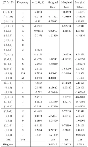
Accordingly, we classify the 340 observations into 27 categories, some of
which may contain no observations. For Table 4, the data is actually not
ran-domized: we label Type 1 twins before Type 2 twins according to their orders
in the original data. Column 2 lists the frequency for each category of (U, M, E)
315
in Column 1.
Our purpose is to quantify the income differential due to the schooling
dif-ferential only, U and M remaining unchanged. Let v(U, M, E) be the average
difference of hourly wages between Type 1 twins and Type 2 twins in the cat-egory (U, M, E). The difference comes from the values of U, M, E, as well as
sampling error. Column 3 of Table 4 lists thev for the non-randomized dataset.
For the category (U, M,1), the marginal gain and effect isv(U, M,1)−v(U, M,0); the effect is only due to the difference inEi, plus a random error. For the
cat-egory (U, M,−1), the marginal loss and effect isv(U, M,0)−v(U, M,−1). For
the category (U, M,0), the marginal gain is v(U, M,0)−v(U, M,−1) and the marginal loss is v(U, M,1)−v(U, M,0); we average them for calculating the
marginal effect, i.e.
[v(U, M,0)−v(U, M,−1)] + [v(U, M,1)−v(U, M,0)]
2 =
v(U, M,1)−v(U, M,−1)
2 .
The last three columns of Table 4 list the marginal gain, loss, and effect for the
non-randomized dataset. The last row is the weighted marginal gain, loss and
calculated as:
h
1(−11.791) + 2(−3.4492) +· · ·+ 2(4.7643) + 1(−.2133)i/338 = 2.7995.
Repeating the above calculations for a large number of randomized datasets,
we obtain a large set of frequency-weighted marginal gain, loss and effect, due
to one or more years of schooling. Given the average hourly wage $14.44 in
1993, we find that both mean and median wage increase is about 18.3%. The
320
results are consistent with, though slightly lower than, those from the marginal
[image:19.612.162.451.312.525.2]gain and marginal loss. The statistics are summarized in Table 1.
Table 1: Marginal Gain, Loss and Effect of 1+ Years of Schooling (in %, exceptα)
Mean Median Std. Dev .95 Confidence Band
marginal effect 18.2879 18.2833 1.30667 [15.8921, 20.7155]
marginal gain 18.8138 18.7626 4.30053 [10.5990, 27.2509]
marginal loss 18.7867 18.7543 4.28981 [10.5758, 27.1039]
bias ratioα .001343 .000459 .448105 [-.864527, .867927]
Figure 3: Multi-modal Effects of Additional Schooling Years on Wage
Though the estimated endowment bias ratio has slightly positive mean and
median, it is not significantly different from zero, showing no enough evidence
of endowment bias. Interestingly, the effects show a multi-modal distribution
325
(Figure 3) with modes at 17.7% and 19.2%, respectively. Unlike a regression
method, our calculation allows heterogeneous effects from the other explanatory
[image:19.612.156.457.316.403.2]approach addresses the asymmetric sides of the marginal effects and the
non-parametric method assumes less assumptions than a regression one. Interested
330
readers can re-categorize theEivariable to find the effects of other educational
differential.
6. Discussions, Variations, and Applications
Given the evaluation ˜ψ, we select those variables with large D-value ˜ψi in
modeling the data generating process. The selected variables, however, may not
335
have the best collective performance under certain criterion. The model with
the best performance under the criterion, on the other hand, does not
neces-sarily produce the best performance under other criteria. This dilemma leads
us to evaluate the variables not in one specific model context, but in modeling
scenarios specified by a prior distribution. Moreover, as a tool for multi-criteria
340
decision analysis, our valuation approach seeks the balance between data fitting,
prediction, and other criteria. Depending on specific contexts, similar ideas can
be applied to other areas of economics, finance, political science, and statistics
without substantial changes.
6.1. Structural valuation 345
In a real valuation situation, it could be proper to specify a context-specific
prior µ; for example, in a voting, let |S| have a uniform distribution on the
integers in ⌊n/4,3n/4⌋, rather than on the integers in [0, n]. This can also be
readily done by placing restrictions onµ; for example, if playersiandj would
never cooperate in the voting, then the probability ofij ∈ Sshould be zero.
350
Though analytic formula is unlikely available for ψ[v;µ] under a restricted µ,
Monte Carlo method is generally feasible. In the Monte Carlo simulations, we
simply ignore the restricted cases, randomly generated from Ω or aµ∈ F.
6.2. Unemployment Compensation
LetN be the labor force (either employed or seeking for employment) of an
355
collectively by T. Then, a fair and efficient rule to distribute unemployment
benefits could be the solution of ψ[v;µ] such that µ ∈ F and
n
P
i=1
ψi[v;µ] =
max
T v(T), instead ofv(N). Under the efficiency assumption of the labor market,
the employed Sis expected to maximize the social welfare of the nation; thus
360
the distribution rule solves
n
P
i=1
[image:21.612.129.458.136.339.2]ψi[v;µ] = E[v(S)].
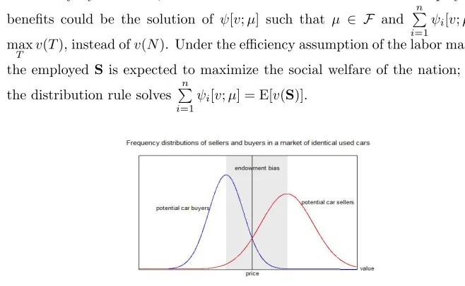
Figure 4: The price is determined at the intersection of frequency plots
6.3. A Theory of Price
Consider a market of identical used cars (or a secondary market of a stock
or bond). There are two groups of market participants: potential sellers and
potential buyers. Each group has its own frequency distribution with
heteroge-365
neous valuation about the car. The value of a car to the potential sellers is the
marginal gain; to the potential buyers, it is the marginal loss. In Figure 4, the
frequence plots intersect at a price where the demand quantity equals to the
supply quantity.
6.4. Power Index in a Ternary Voting System 370
Let us study a ternary voting rule in which a voter has only two choices,
but v(S) has three outcomes: passed, failed, or dropped. Here Sdenotes the
random coalition of voters who vote for the bill.
Letτ be a random ordering of all voters. In this ordering, there is exactly
one pivotal voter i such that he changes the outcome v(Ξτ
i), but N \Ξτi \i
375
no longer changes the outcome v(Ξτ
i ∪i). The chance of being pivotal in all
6.5. Value of a CoalitionZ
If N is a firm, a coalition Z could be the sales group or the R&D team.
We treat coalition Z as an indivisible entity; and there are many value-added
opportunities forZand the rest of the firm. For a value ofZ, a natural extension
to the D-valueψi is
E [v(S∪Z)−v(S\Z)]
6.6. Value of Integration or M&A
Assume two disjoint firms M andN. We consider the potential integration
betweenM andN. To evaluate the integration, one could work from the added
value between their coalitions:
E[v(X∪Y)−v(X)−v(Y)]
where randomX⊆N andY⊆M are potential cooperating coalitions.
380
6.7. Value of Substitution
Ifi∈S, theni’s position could be replaced by some other player, sayj, in
N\S. So we have the added value
v(S∪j\i)−v(S).
Dually, if i 6∈ S, then i could substitute for a player, say j, in S. This
substitution gives an added value:
v(S∪i\j)−v(S).
6.8. Analysis of Variance
In regressingY on the variables inT by a linear model, we let v(T) be the
variance ofY explained by T. Decomposition of v(N)−v(∅) by the Shapley
value provides a specific share each variable contributes to modelingY using all
385
6.9. Outliers Detection
In detecting outliers observations, one could apply the D-value ˜ψito evaluate
the overall performance of each observation. For example, consider the MCD
estimator of robust covariance (cf Rousseeuw, 1985). Among all covariances of
390
subsamples of a given size, the MCD estimator has the minimum determinant.
We letN be the full sample of observations andT be a subsample. Let v(T)
be the determinant of the covariance of the subsampleT. We can reasonably
assume no discrimination on any subsample among all subsamples of the same
size. A binomial(n, p) prior withp∈[.9, .99] could be a good choice for the size
395
of non-outliers observations.
6.10. Continuous Categorization
In the empirical study of schooling years, we replace the binary classification
with an ordered ternary one. In a more generic situation, we may assume a
continuous random vectorX= (X1,· · ·, Xn)′∈Rnand a differentiable function
400
v:Rn →R. Letµbe the distribution ofX. In this setting, the marginal effect
is represented by a partial derivative and the corresponding valuation of variable
Xi is
ψi[v;µ] = E
dv(X)
dxi
=
Z
(x1,···,xn)∈Rn
dv(x1,· · ·, xn)
dxi
dµ (12)
in contrast with (2) and the Aumann-Shapley value (Aumann and Shapley,
1974). All interdependence, restrictions, and uncertainty assumption aboutX
405
are contained in the distributionµ.
Given a sample ofX1,· · ·, Xn and the valuev at the sample observations,
we may use a multivariate empirical distribution ˆµto fit the distributionµand
apply a multivariate differentiable function ˆvto fitv. Finally, formula (12) with
µ = ˆµ and v = ˆv estimates variable Xi’s relative importance in modeling Y
410
References
[1] M. Arellano, S. Bond,Some Tests of Specification for Panel Data: Monte
Carlo Evidence and an Application to Employment Equations, Rev. Econ.
Stud. 58 (1991), 277-297.
415
[2] O. Ashenfelter, A. Krueger,Estimates of the economic return to Schooling
from a new sample of twins, Amer. Econ. Rev. 84(1994), 1157-1173.
[3] O. Ashenfelter, C. Rouse,Income, schooling, and ability: evidence from a
new sample of identical twins, Quart. J. Econ. 113(1998), 253-284.
[4] R.J. Aumann, L.S. Shapley,Values of Non-Atomic Games. Princeton
Uni-420
versity Press, Princeton, NJ (1974).
[5] J.F. Banzhaf,Weighted voting doesn’t work: a mathematical analysis,
Rut-gers Law Rev. 19(1965), 317-343.
[6] G.E.P. Box,Science and Statistics, J. of Amer. Stat. Assoc. 71(1976),
791-799.
425
[7] N. Budina, B. Gracia, X. Hu, S. Saksonovs,Recognizing the Bias: Financial
Cycles and Fiscal Policy, IMF Working Paper No. 15/246 (2015).
[8] M. Clyde, E. I. George, Model Uncertainty, Statistical Science 19(2004),
81-94.
[9] F. Devicienti,Shapley-value decomposition of changes in wage distributions: 430
a note, J. Econ. Inequal 8(2010), 35-45.
[10] D.A. Freedman,A Note on Screening Regression Equations, Amer.
Statis-tician 37(1983), 152-155.
[11] E.I. George, R.E. McCulloch,Approaches for Bayesian variable selection,
Statistica Sinica 7(1997), 339-373.
435
[12] U. Gromping,Estimators of relative importance in linear regression based
[13] X. Hu, Value of Loss in n-Person Games, UCLA Comput. Appl. Math.
Reports 02-53 (2002).
[14] X. Hu,An asymmetric Shapley-Shubik power index, Intl. J. Game Theory
440
34(2006), 229-240.
[15] O. Israeli, A Shapley-based decomposition of the R-Square of a linear
re-gression, J. Econ. Inequal 5(2007), 199-212.
[16] S. Lipovetsky, M. Conklin,Analysis of regression in game theory approach,
Appl. Stoch. Models in Business Industry 17(2001), 319-330.
445
[17] N. Megiddo, On Finding Additive, Superadditive and Subadditive
Set-Function Subject to Linear Inequalities, RJ 6329 (61998) 7/11/88,
Com-puter Science/Nathematics, IBM Almaden Research Center, San Jose,
Cal-ifornia.
[18] D. Monderer, D. Samet,Variations on the Shapley Value. In: R.J. Aumann
450
and S. Hart (eds) Handbook of Game Theory, vol 2, Chapter 54 (2002),
pp.2055-2076. Elsevier Science, Netherlands.
[19] R.B. O’Hara, M.J. Sillanpaa, A Review of Bayesian Variable Selection
Methods: What, How and Which, Bayesian Analysis 4(2009), 85-118.
[20] P.J. Rousseeuw, Multivariate estimation with high break-down point. In:
455
W. Grossmann et al. (eds.) Mathematical Statistics and Applications, vol.
B(1985), pp.283-297. Akademiai Kiado, Budapest.
[21] L.S. Shapley,A value for n-person games. In: H.W. Kuhn and A.W. Tucker
(eds.) Contributions to the Theory of Games, Annals of Math. Studies, vol.
28 (1953), pp.307-317. Princeton University Press, Princeton, New Jersey.
460
[22] E. Winter,The Shapley Value. In: R.J. Aumann and S. Hart (eds)
Hand-book of Game Theory, vol 2, Chapter 53 (2002), pp.2025-2054. Elsevier
Appendix
For notational simplicity, we assume that v is 1-dimensional set function v :
465
2N →Rin the proofs.
A1. Proof of Theorem 1
Fort = 0,1,· · ·, n, let δt
def
= P
|T|=t
PT, the probability of |S|=t. As µ∈ F,
PT =
(|T|)!(n−|T|)!
n! δ|T|. For any fixedi∈N, we write (1) as
ψi[v;µ] = P T∋i
PT[v(T)−v(T\i)] +
P
Z6∋i
PZ[v(Z∪i)−v(Z)]
Q=T\i
= P
T∋i
PTv(T)−
P
Q6∋i
PQ
∪iv(Q) +
P
Z6∋i
PZ[v(Z∪i)−v(Z)]
= P
T∋i
PTv(T) +
P
Z6∋i
PZv(Z∪i)−
P
Z6∋i
[PZ +PZ∪i]v(Z)
T=Z∪i
= P
T∋i
PTv(T) +
P
T∋i
P
T\iv(T)−
P
Z6∋i
[PZ+PZ∪i]v(Z)
= P
T∋i
v(T)[PT +PT\i]−
P
T6∋i
v(T)[PT +PT∪i].
(13)
Therefore, By (3)
470
v(N)−v(∅) = P
i∈N
ψi[v;µ]
= P
i∈N
P
T∋i
v(T)[PT +PT\i]−
P
i∈N
P
T6∋i
v(T)[PT +PT∪i]
= P
T⊆N
v(T)P
i∈T
[PT +PT\i]−
P
T⊆N
v(T)P
i6∈T
[PT +PT∪i]
= P
T⊆N
v(T)
"
|T|PT +
P
i∈T
PT
\i−(n− |T|)PT −
P
i6∈T
PT
∪i
#
= P
T⊆N
v(T)
"
(2|T| −n)PT +
P
i∈T
PT
\i−
P
i6∈T
PT
∪i
#
.
(14)
We compare the coefficients ofv(N) andv(∅) in (14) to get
nδn+δn−1= 1, nδ0+δ1= 1.
(15)
For anyT such that T 6=N and T 6=∅, the coefficients ofv(T) in (14) imply
that
(2|T| −n)PT =
X
i6∈T
PT
∪i−
X
i∈T
PT
Let|T|=t, 1≤t≤n−1, and rewrite the above equation in terms ofδ’s,
(2t−n)t!(n−t)!
n! δt = (n−t)
(t+ 1)!(n−t−1)! n! δt+1−t
(t−1)!(n−t+ 1)! n! δt−1.
Or simply,
(2t−n)δt= (t+ 1)δt+1−(n−t+ 1)δt−1. (16) By (15), (16) and Pn
t=0
δt= 1, we haven+ 2 linear equations ofn+ 1 unknowns,
n 1
n 2−n −2
n−1 4−n −3
. .. ... ...
2 n−2 −n
1 n
1 1 1 · · · 1 1 1
δ0 δ1 δ2 .. .
δn−2
δn−1
δn = 1 0 0 .. . 0 1 1 .
The rank of the (n+ 2)×(n+ 1) coefficient matrix is at least n, due to
the fact that the submatrix of the first ncolumns and the middle nrows has
determinant n! 6= 0. It is not hard to verify that the general solution to the
475
system of equations is
δt=
1
n+ 1+ (−1)
t n t
η (17)
for some indeterminateη. Anyη with |η| ≤ min 0≤s≤n
s!(n−s)! (n+1)! =
(⌊n+1 2 ⌋)!(n−⌊
n+1 2 ⌋)!
(n+1)!
guarantees non-negativeδt’s. Thus, for anyT ⊆N,
PT =
(|T|)!(n− |T|)!
(n+ 1)! + (−1)
|T|η.
Therefore, for anyT withi∈T,
PT +PT\i =
(|T| −1)!(n− |T|)!
n! , (18)
and for anyT withi6∈T,
PT +PT∪i =
(|T|)!(n− |T| −1)!
Finally, we plug (18) and (19) into (13),
ψi[v;µ] = P T∋i
(|T|−1)!(n−|T|)!
n! v(T)−
P
T6∋i
(|T|)!(n−|T|−1)!
n! v(T)
Z=T∪i
= P
T∋i
(|T|−1)!(n−|T|)!
n! v(T)−
P
Z∋i
(|Z|−1)!(n−|Z|)!
n! v(Z\i)
T=Z
= P
T⊆N
(|T|−1)!(n−|T|)!
n! [v(T)−v(T\i)] = Ψi[v].
(20)
A2. Proof of Corollary 1 480
If PT =
(|T|)!(n−|T|)!
(n+1)! + (−1)|T|η, clearly µ ∈ F. Furthermore, we repeat (18)−(20) to getψ[v;µ] = Ψ[v].
A3. Proof of Theorem 2
If PT =
1
2n + (−1)|T|η for any T, thenPT +PT\i =PT +PT∪j =
1 2n−1 for
anyi∈T and anyj 6∈T. By (13),
ψi[v;µ] = P T∋i
1
2n−1v(T)− P
T6∋i
1 2n−1v(T)
Z=T∪i
= 1
2n−1 P
T∋i
v(T)− 1 2n−1
P
Z∋i
v(Z\i)
Z=T
= 2n1−1 P
T∋i
[v(T)−v(T\i)] =bi[v].
On the contrary, ifψ[v;µ] =b[v], then for any i,
ψi[v;µ] =
1 2n−1
X
T
[v(T)−v(T\i)] = 1 2n−1
X
T∋i
v(T)− 1
2n−1
X
T6∋i
v(T).
By (13),
PT +PT\i =
1
2n−1, for any i∈T;
PT +PT∪i =
1
2n−1, for any i6∈T.
(21)
Without loss of generality, letP∅ =
1
2n +η for someη with|η| ≤
1
2n. In (21),
485
letT =iand we get
PT =
1
2n−1 −P∅= 1
2n + (−1)
|T|η (22)
for anyT with|T|= 1. Let us assume the above identity holds for allT’s with
|T|=tand consider anyZ with|Z|=t+ 1. Pick ani∈Z and apply (21),
PZ =
1
2n−1 −PZ\i =
1 2n−1 −
1
2n + (−1) tη
= 1
2n + (−1)
|Z|η.
This shows (22) is also true forZ with|Z|=t+ 1. By mathematical induction,
A4. Proof of Theorem 3
Ifµ∈ F and|S|has a binomial distribution with parameters nand p, then
PT =
δ|T|
n
|T|
=
n
|T|
p|T|(1−p)n−|T|
n
|T|
=p|T|(1−p)n−|T|.
Next,
ψi[v;µ] = P T∋i
PT[v(T)−v(T\i)] +
P
Z6∋i
PZ[v(Z∪i)−v(Z)]
T=Z∪i
= P
T∋i
PT[v(T)−v(T\i)] +
P
T∋i
P
T\i[v(T)−v(T\i)]
= P
T∋i
p|T|(1−p)n−|T|+p|T|−1(1−p)n−|T|+1
[v(T)−v(T\i)]
= P
T∋i
p|T|−1(1−p)n−|T|[v(T)−v(T\i)].
From the above, we also see
γi[v;µ] = P T∋i
p|T|(1−p)n−|T|[v(T)−v(T\i)] =pψ
i[v;µ],
λi[v;µ] = P T∋i
p|T|−1(1−p)n−|T|+1[v(T)−v(T\i)] = (1−p)ψ
A5. Proof of Lemma 1 490
κi = E
v(S)−v(S\i)
−E
v(S∪i)−v(S)
= P
T∋i
PT
v(T)−v(T\i)
−P
Z6∋i
PZ
v(Z∪i)−v(Z)
=
" P
T∋i
PTv(T) +
P
Z6∋i
PZv(Z)
#
−P
T∋i
PTv(T\i)−
P
Z6∋i
PZv(Z∪i)
Q=Z∪i
= P
T
PTv(T)−
P
T∋i
PTv(T\i)−
P
Q∋i
P
Q\iv(Q) Z=T\i
= P
T
PTv(T)−
P
Z6∋i
P
Z∪iv(Z)−
P
Q
P
Q\iv(Q) +
P
Q6∋i
P
Q\iv(Q)
= P
T
h
PT −PT\i
i
v(T)−P
Z6∋i
P
Z∪iv(Z) +
P
Q6∋i
PQv(Q)
= P
T
h
PT −PT\i
i
v(T)−P
Z
P
Z∪iv(Z) +
P
Z∋i
P
Z∪iv(Z) +
P
Q6∋i
PQv(Q)
= P
T
h
PT −PT\i−PT∪i
i
v(T) +
" P
Z∋i
PZv(Z) +
P
Q6∋i
PQv(Q)
#
= P
T
h
PT −PT\i−PT∪i
i
v(T) +P
T
PTv(T)
= P
T
h
2PT −PT∪i−PT\i
i
v(T).
A6. Proof of Theorem 4
If PT =
1
2n for any T, then 2PT −PT∪i−PT\i = 0 for any i and T. By
Lemma 1,
κi[v;µ] =
X
T
h
2PT −PT∪i−PT\i
i
v(T) =X
T
0∗v(T) = 0.
On the contrary, if κ[v;µ] = 0, then Lemma 1 implies that 2PT −PT∪i −
PT
\i = 0 for anyiandT. We let the size ofT run from 1 ton:
1. IfT =i, then 2Pi−Pi
∪i−Pi\i = 0, showingPi=P∅ for anyi.
2. If T =ij with i 6= j, then 2P
ij −Pij∪i −Pij\i = 0, showing Pij =
P
j =P∅ for anyi6=j.
3. Let us assume thatPZ =P∅ for anyZ with|Z|=t. For any T with
|T|=t+ 1, we pick anifromT and apply the relation 2PT −PT∪i−
PT
\i = 0, showingPT =PT\i=P∅.
By mathematical induction, we conclude thatPT =P∅ for anyT. As P
T
PT = 1,
495
PT =
A7. Proof of Theorem 5
Forµ∈ F,PT =
(|T|)!(n−|T|)!δ|T|
n! whereδtis the probability of |S|=t. We
first simplify the total bias forµ∈ F.
P
i
γi[v;µ] = P i
P
T∋i
PT[v(T)−v(T\i)]
= P
T6=∅
(|T|)!(n−|T|)!δ|T| n!
P
i∈T
[v(T)−v(T\i)].
P
i
λi[v;µ] = P i
P
T6∋i
PT[v(T∪i)−v(T)]
Z=T∪i
= P
i
P
Z∋i
PZ
\i[v(Z)−v(Z\i)]
= P
Z6=∅
(|Z|−1)!(n−|Z|+1)!δ|Z|−1 n!
P
i∈Z
[v(Z)−v(Z\i)].
Then,
X
i
κi=
X
T6=∅
(|T| −1)!(n− |T|)!(|T|δ|T|−(n− |T|+ 1)δ|T|−1)
n!
X
i∈T
v(T)−v(T\i).
(23)
Thus,P
i
κi[v;µ] = 0 if and only if|T|δ|T| = (n− |T|+ 1)δ|T|−1 for anyT 6=∅.
By induction on the size ofT from 1 ton, we have
δ1 = nδ0,
δ2 = n−21δ1=n(n2!−1)δ0, δ3 = n−32δ2=n(n−1)(3!n−2)δ0,
· · · ·
which establishes thatδt= t!(nn−!t)!δ0 for anyt ≥1. Finally, as
n
P
t=0
δt = 1, we
getδ0= 21n; therefore
PT =
(|T|)!(n− |T|)! n! δ|T| =
(|T|)!(n− |T|)! n!
n!
(|T|)!(n− |T|)!δ0= 1 2n.
A8. Proof of Theorem 6 500
By definitions,
πt = t!(n−nt!−1)! P
|T|=t,i6∈T
[v(T∪i)−v(T)]
Z=T∪i
= ((t+1)−1)!(n!n−(t+1))! P
|Z|=t+1,i∈Z
[v(Z)−v(Z\i)]
T=Z
= ((t+1)−1)!(n!n−(t+1))! P
|T|=t+1
P
i∈T
Therefore, ωt ≥ πt if and only if ωt ≥ ωt+1, or equivalently, ωt is a
decreas-ing function of t. In the same fashion, ωt ≥ πt if and only if πt−1 ≥ πt, or
equivalently,πtis a decreasing function of t.
A9. Proof of Theorem 7
IfPT =
(|T|)!(n−|T|)!
(n+1)! andv has diminishing marginality, then
n
P
i=1
κi[v;µ] = P T6=∅
(|T|)!(n−|T|)! (n+1)!
P
i∈T
[v(T)−v(T\i)]
− P
Z6=N
(|Z|)!(n−|Z|)! (n+1)!
P
i6∈Z
v(Z∪i)−v(Z)
T=Z∪i
= Pn
t=1
P
|T|=t
(|T|)!(n−|T|)! (n+1)!
P
i∈T
[v(T)−v(T\i)]
− P
T6=∅
(|T|−1)!(n+1−|T|)! (n+1)!
P
i∈T
v(T)−v(T\i)
=
n
P
t=1
t n+1ωt−
n
P
t=1
P
|T|=t
(|T|−1)!(n+1−|T|)! (n+1)!
P
i∈T
v(T)−v(T\i)
= Pn
t=1
t n+1ωt−
n
P
t=1
n+1−t n+1 ωt=
n
P
t=1 2t n+1ωt−
n P t=1 ωt = n 1 n n P t=1 2t n+1
(ωt)−
1 n n P t=1 ωt n1
n P t=1 2t n+1
which is the sample covariance, multiplied byn, between the series { 2t n+1}nt=1
505
and the series{ωt}nt=1. As n2+1t is increasing intwhileωtis decreasing int, the
sample covariance is non-positive. Therefore,
n
P
i=1
κi[v;µ]≤0.
Ifv is super-additive, then v(∅) = 0 andv is monotone, i.e.,v(S)≤v(T) if
S⊂T (cf Megiddo, 1988). Let
∆1 = P
T6=∅
(|T|)!(n− |T|)!P
i∈T
v(T)−v(T\i)
,
∆2 = P
Z6=N
(|Z|)!(n− |Z|)!P
i6∈Z
v(Z∪i)−v(Z)
.
Note that ∆1equals
P
T6=∅
|T|(|T|)!(n− |T|)!v(T)− P
T6=∅
P
i∈T
(|T|)!(n− |T|)!v(T\i)
Z=T\i
= P
T6=∅
|T|(|T|)!(n− |T|)!v(T)− P
Z6=N
P
i6∈Z
(|Z|+ 1)!(n− |Z| −1)!v(Z)
= P
T6=∅
|T|(|T|)!(n− |T|)!v(T)− P
Z6=N
and ∆2 equals
P
Z6=N
(|Z|)!(n− |Z|)!P
i6∈Z
v(Z∪i)− P
Z6=N
(|Z|)!(n− |Z|)!(n− |Z|)v(Z)
T=Z∪i
= P
T6=∅
(|T| −1)!(n− |T|+ 1)! P
i∈T
v(T)− P
Z6=N
(|Z|)!(n− |Z|)!(n− |Z|)v(Z)
= P
T6=∅
(|T|)!(n− |T|+ 1)!v(T)− P
Z6=N
(|Z|)!(n− |Z|)!(n− |Z|)v(Z).
Thus, ∆1−∆2equals
P
T6=∅
(|T|)!(n− |T|)!(2|T| −n−1)v(T) + P
Z6=N
(|Z|)!(n− |Z|)!(n−2|Z| −1)v(Z)
= n!(n−1)v(N)− P
T6=∅,T6=N
(|T|)!(n− |T|)!v(T)− P
Z6=N,Z6=∅
(|Z|)!(n− |Z|)!v(Z)
T=N\Z
= n!(n−1)v(N)− P
T6=∅,T6=N
(|T|)!(n− |T|)!v(T)− P
T6=∅,T6=N
(n− |T|)!(|T|)!v(N\T)
= n!(n−1)v(N)− P
T6=∅,T6=N
(|T|)!(n− |T|)!v(T) +v(N\T)
≥ n!(n−1)v(N)− P
T6=∅,T6=N
(|T|)!(n− |T|)!v(N)
= n!(n−1)v(N)−
n−1
P
t=1
P |T|=t
(|T|)!(n− |T|)!v(N)
= n!(n−1)v(N)−
n−1
P
t=1
n!v(N) = 0.
Finally, whenµis the benchmark distribution for the Shapley value,
n
X
i=1
κi[v;µ] =
∆1 (n+ 1)! −
∆2 (n+ 1)! =
∆1−∆2 (n+ 1)! ≥0
for the super-additivev.
A10. Proof of Theorem 8
Usingγi[v;µ] and λi[v;µ] in the proof of Theorem 3,
κi[v;µ] = P T∋i
p|T|(1−p)n−|T|[v(T)−v(T\i)]
−P
T∋i
p|T|−1(1−p)n−|T|+1[v(T)−v(T\i)] = (2p−1)P
T
p|T|−1(1−p)n−|T|[v(T)−v(T\i)].
By Theorem 3,α= 2p−1. Finally, by (6),
˜
ψi[v;µ] = (1−(2p−1))P T∋i
p|T|(1−p)n−|T|[v(T)−v(T \i)]
+(1 + (2p−1))P
T∋i
p|T|−1(1−p)n−|T|+1[v(T)−v(T \i)]
= 4 P
T∋i
A11. Proof of Theorem 10 510
As the ordering τ has a uniform distribution over Ω, each ordering has a
probability 1
n!. Moreover, there are (|Ξτi|)! permutations in Ξiτand (n−1−|Ξτi|)!
permutations inN\Ξτ
i \i, the set of elements preceded byiin the orderingτ.
Thus, the probability of Ξτ i =T is
(|Ξτ
i|)!(n−1−|Ξτi|)!
n! =
(|T|)!(n−1−|T|)!
n! . Using the
double expectation formula, we have
E[ ˜φτ
i] = E
h
E[ ˜φτ i |Ξτi]
i
= P
T6∋i
Prob(Ξτ i =T)E
h
˜ φτ
i | Ξτi =T
i
= P
T6∋i
(|T|)!(n−1−|T|)!
n!
n!(PT+PT∪i) (|T|)!(n−|T|−1)!
v(T∪i)−v(T)
= P
T
(PT +PT∪i)
v(T∪i)−v(T)
= P
T
PT
v(T∪i)−v(T)
+P
T
P
T∪i
v(T∪i)−v(T)
Z=T∪i
= λi[v;µ] +P Z
PZ
v(Z)−v(Z\i)
= λi[v;µ] +γi[v;µ] =ψi[v;µ].
The above proof already implies (9). For the Shapley value, let us apply (4)
withη= 0,
n!P Ξτ
i∪i
(|Ξτ
i|)!(n−|Ξτi|−1)!
=
n!(|i∪Ξτi|)!(n−|i∪Ξτi|)!
(n+1)! (|Ξτ
i|)!(n−|Ξτi|−1)!
=
1+|Ξτ i|
n+1
,
n!PΞτi
(|Ξτ
i|)!(n−|Ξτi|−1)!
=
n!(|Ξτi|)!(n−|Ξτi|)!
(n+1)! (|Ξτ
i|)!(n−|Ξτi|−1)!
=
n−|Ξτ i|
n+1
.
For the unbiased Shapley value, the right-hand side of (11) is
4EnEh(|Ξτi|+1)(n−|Ξ τ i|)
(n+1)(n+2) [v(Ξτi ∪i)−v(Ξτi)]|Ξτi
io
= 4 P
T6∋i
Prob(Ξτ
i =T) E
h(|Ξτ
i|+1)(n−|Ξτi|)
(n+1)(n+2) [v(Ξτi ∪i)−v(Ξτi)]|Ξτi =T
i
= 4 P
T6∋i
(|T|)!(n−1−|T|)!
n!
(|T|+1)(n−|T|)
(n+1)n+2) [v(T ∪i)−v(T)]
Z=T∪i
= 4 P
Z∋i
(|Z|)!(n−|Z|+1)!
Table 2: Multivariate Shapley Value and its Percentage (in Parenthesis)
Variable R-squared Squared t-stat Abs t-stat MSE: MSE:
dynamic static
Ei,t−1 0.00331*** 390.90*** 19.630*** 0.0044*** 0.0073***
(42.31) (48.67) (29.39) (17.01) (27.26)
Ei,t−2 0.00040* 29.64 5.066* 0.0035** 0.0025*
( 5.15) ( 3.69) ( 7.58) (13.57) ( 9.45)
Wi,t 0.00057* 59.76* 7.578** 0.0009 0.0009
( 7.27) ( 7.44) (11.35) ( 3.50) ( 3.34)
Wi,t−1 0.00010 12.15 3.088 0.0009 0.0009
( 1.34) ( 1.51) ( 4.62) ( 3.31) ( 3.50)
Wi,t−2 0.00002 1.79 1.056 0.0021* 0.0019*
( 0.20) ( 0.22) ( 1.58) ( 8.30) ( 6.95)
Ki,t 0.00212*** 215.47*** 14.424*** 0.0048*** 0.0048***
(27.15) (26.82) (21.60) (18.69) (17.78)
Ki,t−1 0.00077* 55.28* 5.914* 0.0025* 0.0025*
( 9.85) ( 6.88) ( 8.85) ( 9.68) ( 9.30)
Ki,t−2 0.00020 12.93 2.821 0.0026** 0.0022*
( 2.53) ( 1.61) ( 4.22) (10.15) ( 8.19)
Yi,t 0.00015 11.70 3.126 0.0007 0.0007
( 1.86) ( 1.46) ( 4.68) ( 2.57) ( 2.58)
Yi,t−1 0.00012 9.60 2.568 0.0011 0.0012
( 1.54) ( 1.20) ( 3.84) ( 4.47) ( 4.42)
Yi,t−2 0.00006 4.03 1.517 0.0023* 0.0019*
( 0.81) ( 0.50) ( 2.27) ( 8.76) ( 7.23)
Table 3: Unbiased Multivariate Shapley Value and its Percentage (in Parenthesis)
Variable R-squared Squared t-stat Abs t-stat MSE: MSE:
dynamic static
Ei,t−1 0.00319*** 387.57*** 19.591*** 0.0038*** 0.0064***
(43.07) (48.85) (29.43) (19.79) (30.80)
Ei,t−2 0.00036 28.70 5.026* 0.0023** 0.0018*
( 4.91) ( 3.62) ( 7.55) (12.12) ( 8.49)
Wi,t 0.00057* 60.92* 7.617** 0.0010* 0.0010
( 7.70) ( 7.68) (11.44) ( 5.05) ( 4.61)
Wi,t−1 0.00011 12.62 3.121 0.0006 0.0007
( 1.47) ( 1.59) ( 4.69) ( 2.94) ( 3.25)
Wi,t−2 0.00002 1.88 1.072 0.0014* 0.0012*
( 0.22) ( 0.24) ( 1.61) ( 7.26) ( 5.92)
Ki,t 0.00201*** 212.08*** 14.370*** 0.0040*** 0.0040***
(27.07) (26.73) (21.59) (20.78) (19.20)
Ki,t−1 0.00068* 52.39* 5.814* 0.0017* 0.0017*
( 9.18) ( 6.60) ( 8.73) ( 8.96) ( 8.41)
Ki,t−2 0.00017 12.26 2.775 0.0018* 0.0015*
( 2.33) ( 1.55) ( 4.17) ( 9.36) ( 7.04)
Yi,t 0.00013 11.61 3.121 0.0004 0.0005
( 1.82) ( 1.46) ( 4.69) ( 2.29) ( 2.38)
Yi,t−1 0.00011 9.53 2.565 0.0007 0.0008
( 1.49) ( 1.20) ( 3.85) ( 3.72) ( 3.78)
Yi,t−2 0.00005 3.82 1.498 0.0015* 0.0013*
( 0.73) ( 0.48) ( 2.25) ( 7.74) ( 6.12)
ˆ
α -.227 -.111 -.057 -.508 -.477
Table 4: Trichotomized Marginal Gain, Loss and Effect in the Non-Randomized Data
(U, M, E) Frequency v(U, M, E) Marginal Marginal Marginal
Gain Loss Effect
(-1,-1,-1) 1 5.4173 -11.1971 -11.1971
(-1,-1,0) 2 -5.7798 -11.1971 4.29880 -3.44920
(-1,-1,1) 2 -1.481 4.29880 4.29880
(-1,0,-1) 12 -7.8986 6.97910 6.97910
(-1,0,0) 15 -0.91951 6.97910 -4.31830 1.33040
(-1,0,1) 4 -5.2378 -4.31830 -4.31830
(-1,1,-1) 0 .
(-1,1,0) 0 .
(-1,1,1) 2 4.7123
(0,-1,-1) 1 -4.1197 1.64230 1.64230
(0,-1,0) 5 -2.4774 1.64230 -4.82210 -1.58990
(0,-1,1) 8 -7.2995 -4.82210 -4.82210
(0,0,-1) 45 -2.9165 3.63000 3.63000
(0,0,0) 133 0.7135 3.63000 3.34890 3.48950
(0,0,1) 51 4.0624 3.34890 3.34890
(0,1,-1) 4 -4.6898 2.13620 2.13620
(0,1,0) 8 -2.5536 2.13620 -1.00840 0.56390
(0,1,1) 4 -3.562 -1.00840 -1.00840
(1,-1,-1) 2 2.6511 -0.53780 -0.53780
(1,-1,0) 1 2.1133 -0.53780 -4.87170 -2.70480
(1,-1,1) 1 -2.7584 -4.87170 -4.87170
(1,0,-1) 13 -2.4809 5.72810 5.72810
(1,0,0) 13 3.2472 5.72810 -1.05760 2.33530
(1,0,1) 9 2.1896 -1.05760 -1.05760
(1,1,-1) 1 -8.0136 9.74190 9.74190
(1,1,0) 2 1.7283 9.74190 -0.21330 4.76430
(1,1,1) 1 1.515 -0.21330 -0.21330
Total 340 259 258 338