Topology management protocols in ad hoc wireless sensor networks

(1)

A Dissertation by HO GIL KIM

Submitted to the Office of Graduate Studies of Texas A&M University

in partial fulfillment of the requirements for the degree of DOCTOR OF PHILOSOPHY

December 2007

(2)

A Dissertation by HO GIL KIM

Submitted to the Office of Graduate Studies of Texas A&M University

in partial fulfillment of the requirements for the degree of DOCTOR OF PHILOSOPHY

Approved by:

Chair of Committee, Eun Jung Kim Committee Members, Valerie E. Taylor

Rabi N. Mahapatra Deepa Kundur Head of Department, Valerie E. Taylor

December 2007

(3)

ABSTRACT

Topology Management Protocols in Ad Hoc Wireless Sensor Networks. (December 2007)

Ho Gil Kim, B.S., Korea Military Academy, Korea; M.S., Younsei University, Korea

Chair of Advisory Committee: Dr. Eun Jung Kim

A wireless sensor network (WSN) is comprised of a few hundred or thousand au-tonomous sensor nodes spatially distributed over a particular region. Each sensor node is equipped with a wireless communication device, a small microprocessor, and a battery-powered energy source. Typically, the applications of WSNs such as habitat monitoring, fire detection, and military surveillance, require data collection, process-ing, and transmission among the sensor nodes. Due to their energy constraints and hostile environments, the main challenge in the research of WSN lies in prolonging the lifetime of WSNs.

In this dissertation, we present four different topology management protocols for K-coverage and load balancing to prolong the lifetime of WSNs.

First, we present a Randomly Ordered Activation and Layering (ROAL) protocol forK-coverage in a stationary WSN. The ROAL suggests a new model of layer cov-erage that can construct aK-covered WSN using the layer information received from its previously activated nodes in the sensing distance. Second, we enhance the fault tolerance of layer coverage through a Circulation-ROAL (C-ROAL) protocol. Us-ing the layer number, the C-ROAL can activate each node in a round-robin fashion during a predefined period while conserving reconfiguration energy. Next, Mobility Resilient Coverage Control (MRCC) is presented to assureK-coverage in the presence

(4)

of mobility, in which a more practical and reliable model forK-coverage with nodal mobility is introduced. Finally, we present a Multiple-Connected Dominating Set (MCDS) protocol that can balance the network traffic using an on-demand routing protocol. The MCDS protocol constructs and manages multiple backbone networks, each of which is constructed with a connected dominating set (CDS) to ensure a con-nected backbone network. We describe each protocol, and compare the performance of our protocols with Dynamic Source Routing (DSR) and/or existing K-coverage algorithms through extensive simulations.

The simulation results obtained by the ROAL protocol show thatK-coverage can be guaranteed with more than 95% coverage ratio, and significantly extend network lifetime against a given WSN. We also observe that the C-ROAL protocol provides a better reconfiguration method, which consumes only less than 1% of the reconfigura-tion energy in the ROAL protocol, with a greatly reduced packet latency. The MRCC protocol, considering the mobility, achieves better coverage by 1.4% with 22% fewer active sensors than that of an existing coverage protocol for the mobility. The results on the MCDS protocol show that the energy depletion ratio of nodes is decreased consequently, while the network throughput is improved by 35%.

(5)

(6)

ACKNOWLEDGMENTS

Dr. Eun Jung Kim, my academic advisor, taught me the lesson I needed most to learn. I am grateful to her stimulating suggestions and encouragement in all the times of research for and writing of this dissertation. I could learn her boundless energy dedicated to research and our lab students. The high standards she has imparted to me will guide my research efforts my whole life long. I would like to thank Dr. Valerie E. Taylor, my dissertation committee member, for helpful discussion on the way of data acquisition and presentation. I improved the results of this dissertation via her great idea. Dr. Rabi N. Mahapatra, my other committee member, has offered sound advice over the years. I have been incredibly fortunate to have had a creative discussion with him. I also wish to thank Dr. Deepa Kundur who is my other committee member. She has given and confirmed the novelty of this research and encouraged me to go ahead with my idea. I have furthermore to thank Dr. Yoon Suk Choi for his helpful advice and support for this dissertation during the presentation of this dissertation.

I am especially grateful for the friendship of Yuho Jin, Manhee Lee and Heungki Lee who are the first members of our lab. They always used to abide with me whenever I need their help. I also thank all our other lab members, Minseon, Inchoon, Sungho, Baik Song, Jay, and James for their helpful work and talk for my research. My former and current colleagues from the Department of Computer Science supported me in the way of technical discussion, advice, and friendship. I profited immensely from my colleagues of Korea Military Academy as well as the worship members from Vision-Mission Church during my study. They have not hesitated to share my pleasure as a brother and friend. I would like to appreciate all of them with my great honor.

(7)

TABLE OF CONTENTS

CHAPTER Page

I INTRODUCTION. . . 1

A. K-coverage Problem . . . 2

B. Load Balancing Problem . . . 3

II ROAL: A RANDOMLY ORDERED ACTIVATION AND LAYERING PROTOCOL FORK-COVERAGE . . . 6

A. Background and Related Work . . . 6

B. The ROAL Protocol . . . 8

1. Basic Idea . . . 8

2. Randomly Ordered Activation (ROA) Algorithm . . . 9

3. Detailed ROAL Protocol . . . 11

a. Initialization Phase (IP) . . . 11

b. Activation Phase (AP) . . . 13

c. Working Phase (WP) . . . 14

C. Experimental Results . . . 15

1. Coverage Evaluation . . . 15

2. Network Performance . . . 20

D. Conclusion . . . 22

III C-ROAL: CIRCULATION-ROAL ENHANCED WITH FAULT-TOLERANCE FOR K-COVERAGE . . . 25

B. Circulation-ROAL Protocol . . . 27

1. Model of Circulation-ROAL (C-ROAL) . . . 28

2. Circulation Rule . . . 29

3. Discussion on Fault Tolerance . . . 32

C. Analysis on Layer Coverage . . . 32

1. Connectivity . . . 33

2. Coverage . . . 36

3. Simulation . . . 36

D. Conclusion . . . 37

IV MRCC: MOBILITY RESILIENT COVERAGE CONTROL FORK-COVERAGE . . . 39

(8)

B. Mobility Model and MRCC Protocol . . . 41

1. Probabilities in Mobility Model . . . 42

a. Probability of Moving In C(a, R), Pm.i . . . 43

b. Probability of Moving Out C(a, R), Pm.o . . . . 45

c. Deciding Wake-up Call . . . 47

2. MRCC Protocol Mechanism . . . 49

3. MRCC Protocol with Wear-out Failures . . . 50

C. Experimental Results . . . 52

D. Conclusion and Future Work . . . 56

V MULTIPLE-CDS TOPOLOGY FOR WIRELESS SENSOR NETWORKS . . . 58

B. Related Work . . . 59

C. Protocol Overview . . . 61

1. Route Discovery in DSR Protocol . . . 61

2. CDS and CDS Layers . . . 63

3. MCDS Topology for DSR Protocol . . . 64

D. MCDS Protocol . . . 66

1. Stage 1: Primitive-Layering (PL) Procedure . . . 67

2. Stage 2. Inter-Layering (IL) Procedure . . . 71

3. Stage 3: Runtime-Layering (RL) Procedure . . . 74

4. Fault Tolerance . . . 78

E. Simulation Environment and Results . . . 78

1. Simulation Setup . . . 78

2. Simulation Results . . . 79

a. Properties of MCDS Structure . . . 79

b. Effect on Load Balancing . . . 81

c. Effect on Network Performance . . . 84

F. Conclusion . . . 86

VI CONCLUSION . . . 95

REFERENCES . . . 97

(9)

LIST OF TABLES

TABLE Page

I Comparisons ofAd vs. A0 and Avg. vs. Ind. Prob. . . 55 II Primitive-Layering Procedure . . . 70 III Simulation Environments and Scenarios . . . 80

(10)

LIST OF FIGURES

FIGURE Page

1 K-Layer Coverage . . . 8

2 Three Possible Scenarios in the ROAL Protocol . . . 12

3 State Transition Diagram for Each Node During One Round . . . 15

4 Ratios of Covered Areas . . . 16

5 Average Coverage Degree . . . 18

6 Number of Working Nodes . . . 19

7 Average Residual Energy with DSR Only . . . 20

8 Residual Energy with the ROAL Protocol . . . 23

9 Packet Delivery Ratio and Average Coverage Degree . . . 24

10 State Transition with Circulation . . . 30

11 Minimum Distance between Two Working Nodes . . . 33

12 Maximum Distance of Two Closest Working Nodes . . . 35

13 Comparison of Energy Consumption for Reconfiguration . . . 37

14 Average Delay Incurred by Reconfiguration . . . 38

15 Probability of Moving In vs. Moving Out . . . 43

16 Pm.i vs. Pm.o . . . 46

17 Probability of Moving In/Out According to Distance of Active Sensor 48 18 State Transition Diagram for Each Sensor in MRCC . . . 49

(11)

20 Comparison of Large (0.25µ) vs. Small (0.05µ) Duty Cycle in the

Long Run . . . 54

21 The Concept of Dominating-And-Connecting (DAC) . . . 64

22 Concept of Layer Communication . . . 65

23 Maximum, Minimum, and Average Number of Layers Constructed via DAC. . . 81

24 Average Number of Elected Nodes in Each Layer via DAC . . . 82

25 Number of Energy-depleted Nodes with 40m Transmission Range . . 87

29 Residual Energy with Transmission Range of 40m . . . 89

33 Delay . . . 91

34 Average Number of Hop Counts. . . 91

35 Overhead of Route Request (RREQ) Packets . . . 92

36 Overhead of Data Packets . . . 92

37 Delivery Ratio with Transmission Range of 40m . . . 93

(12)

CHAPTER I

INTRODUCTION

A wireless sensor network is a wireless network that is comprised of numerous small sensor nodes, each of which is equipped with a radio transceiver, a small microproces-sor, a data memory, a group of sensors, and a battery. With respect to low cost and tiny sensor nodes, recent advances in embedded computing systems have developed a single tiny sensor node, called mote, within a size of 1-inch x 1.5-inch [1], or even a thumb-sized device [2].

Usually, a hundred or a thousand of the tiny sensor nodes are spatially distributed over a remote target area and operate autonomously. The distributed sensor nodes cooperatively collect and transmit sensed data, such as heat, pressure, light, vibra-tions, etc., and a new data regenerated from the raw data, through neighbor nodes. The task of data collection requires a reliable sensing ability, and the data transmis-sion should be guaranteed between any pair of source and destination. Meanwhile, due to the energy constraints and unmanned control, the main challenge in the re-search of WSN is to prolong the lifetime of WSNs for the reliable data collection and transmission. Since the network lifetime of WSN is restricted by the small capacity of a battery, it is a critical issue to minimize the energy consumption of each node without loss of the functionality of WSN including a robust fault tolerating method. In this dissertation, we are interested in the topic of topology management to provide energy efficient and robust WSNs by applying the well-known K-coverage and the load balancing problems. K-coverage is the study to fulfill the reliability of coverage while turning off any redundant node for the sake of energy conservation.

(13)

Load balancing, on the other hand, studies a technique to balance network traffic evenly so that an early energy depletion, along with any hot spot path, will not cause the network to disconnect. Most of the strategies concerning energy conservation fall into the above two categories.

A. K-coverage Problem

The K-coverage of WSNs studies a methodology to ensure that every point in a target area is covered by at least K different working nodes. The set of redundant nodes, then, can sleep until one of the working nodes fails. As a result, theK-covered network can extend the network lifetime without loss of sensing reliability. Hence, the trade-off between the quality of coverage and the number of nodes selected for maintaining the coverage is a critical issue to implement K-coverage algorithm.

A node can determine its eligibility as a working node by calculating the over-lap of its covering area between its working neighbor nodes based on the geographic coordinate and the distance of sensing radius, which is a general approach in most K-coverage algorithms. This approach can provide almost perfect K-coverage; how-ever, it will cause a significant computation and message overhead in a high density network. Furthermore, it can be costly to obtain an exact geographic coordinate using either the Global Positioning System (GPS) or a virtual coordinate retrieval algorithm [3, 4].

We propose Randomly Ordered Activation and Layering (ROAL) protocol for the K-coverage, which can select a set of working nodes locally without any coordinate system. Our decision algorithm in ROAL runs in O(K) computation time and with O(K) message overhead at each node, where K is the degree of coverage. In our extended work of C-ROAL protocol, a more robust and energy-efficient fault-tolerant

(14)

K-coverage algorithm will be introduced.

In the point of nodal mobility, the ROAL and C-ROAL protocols express no concrete idea. For this reason, we study aK-coverage model under the mobile situa-tion. A mobility resilient coverage control (MRCC)K-coverage model is designed to guarantee the K-coverage in the presence of mobility. In this work, we also present the impact of wear-out failures of sensor nodes to the obtained K-coverage.

B. Load Balancing Problem

Load balancing, as explained before, refers to distributing network traffic evenly across a network so that no single path is overwhelmed and the network can remain con-nected as long as possible.

The problem of load balancing in WSNs has been studied through the multipath or distributed routing protocol. The multipath routing protocol aims to discover multiple disjoint paths between any pair of source and destination. The multiple paths discovered are maintained in a memory, i.e., route cache, and can be used either as a backup route for a broken path or to balance network traffic. However, the decision procedure to find an optimal path to balance network traffic using the multiple paths requires additional computational overhead, including managing the current link state such as a residual energy or the amount of usage [5].

On the other hand, a distributed routing scheme is developed for coordinate-based routing protocols, such as GPSR [6], to provide the load balancing. The ge-ographic coordinate in GPSR is used for each forwarding node to select the next hop node closer to the direction of destination. Although GPSR can provide the distributed shortest path routing, it has the same problem related to using the GPS system and could cause a hot spot around an obstacle, i.e., a region unoccupied by

(15)

sensor nodes. Variant new virtual coordinate systems, instead of the geographic coor-dinate system, are proposed to avoid the hot spot problem in GPSR in many previous studies [3, 4, 7, 8].

In this dissertation, we suggest a MCDS protocol to balance the network traf-fic using dynamic source routing (DSR). The suggested protocol uses the concept of connected dominating set (CDS) to build a load-balanced topology unlike the coordinate-based protocols with which a big overhead to abstract a global topology could occur as the node density increases. In addition, our protocol needs no addi-tional overhead to retrieve an optimal path among multiple paths. Instead, sensor nodes proactively construct multiple virtual layers that are composed of a connected dominating nodes, and the constructed multiple layers provide a distributed routing environment for DSR routing protocol.

In Chapter II, we propose the ROAL protocol that introduces a basic concept of layer coverage and a reconfiguration scheme as a method to balance the energy of each node. In Chapter III, we present a circulation method that can substitute each set of working nodes with a set of sleeping nodes instantly, which greatly reduces the energy consumed for the reconfiguration of the ROAL protocol. We also show the analytical model of the expected coverage and connectivity of our layer coverage in this chapter. In Chapter IV, we develop aK-coverage model in the presence of mobility. We derive a model of moving-in and moving-out probability to correctly model the dynamic changes of network with the respect of K-coverage. We also combine a wear-out failure of each node to properly control the working period of individual nodes. In Chapter V, we discuss the MCDS protocol. An heuristic algorithm to construct multiple CDSs is introduced, and the feature of load balancing and network performance with the MCDS protocol is studied against the case where only DSR is used without MCDS. Finally, we conclude our research in Chapter VI by reviewing

(16)

(17)

CHAPTER II

ROAL: A RANDOMLY ORDERED ACTIVATION AND LAYERING PROTOCOL FOR K-COVERAGE

In this chapter, we propose a Randomly Ordered Activation and Layering (ROAL) protocol. Each node under the ROAL protocol can decide its eligibility regarding a given coverage degree K at randomly generated activation time using only the coverage status informed from its neighbor nodes located within its sensing region. A new concept of layer coverage also provides a simple and effective reconfiguration method for energy balancing. The simulation results show that the ROAL protocol can guaranteeK-coverage with more than 95% coverage ratio, which almost closes to the coverage ratio that is achieved using the geographic coordinate. A significantly extended network lifetime is also observed against the original topology of a given network.

The rest of the chapter is organized as follows. In Section A, we discuss the related work and we provide the details of the ROAL protocol in Section B. In Sec-tion C, we present our simulaSec-tion results to analyze the performance of the proposed algorithm, while we conclude our work in Section D.

A. Background and Related Work

The K-coverage problem is the study on the decision for selecting a set of working nodes such that, with K-covered sensor network, any point in an interesting area is monitored by at leastK different sensor nodes. The final goal of the K-coverage is, hence, to prolong the network lifetime using a limited energy budget of sensor nodes without losing the sensing quality.

(18)

deterministic and probabilistic algorithms. The algorithms in the first category [9, 10, 11] aim to monitor as many points as possible with K different active nodes simultaneously. The other approaches [12, 13, 14, 15] provide the requiredK-coverage based on the expected number of observations for each point, moving target during a given time interval, or the whole duration of movements.

As a highly related approach, we show three studies here. Ye et al. [10] proposed the probing environment and adaptive sleeping (PEAS) protocol that can cover and connect a sensor network by activating only one node within a probing radius of a node. They provided an heuristic way to provide a certain degree of coverage, decided by the number of distributed sensors. An integrated analytical model for multi-coverage and connectivity was suggested by Xing et al. [11], where a sensor network isK-covered if and only if all the points within the intersection area formed by all neighboring nodes are covered by K nodes. The main problem with this approach is the time complexity of O(N3_{), where} _N _{is the number of neighboring} nodes. On the other hand, Set K-Cover problem [15] uses a similar concept as our layering algorithm. However, in these studies, the focus is to makeK subsets using all deployed nodes such that each subset covers all area or can take a K-coverage effect by the iterative activation of each subset in a round-robin fashion. In this scheme, each node belongs to one subset, and then each subset is activated one by one. To select nodes efficiently in terms of accuracy, they also use the geographic information. The ROAL protocol suggested here selects only K subsets and the purpose is to guarantee 1-coverage for each layer without using the geographic information.

We apply the probing scheme proposed in PEAS [10] and sentry selection proto-col [16], where each node sends a hello message to check out any other active nodes within its sensing area. If there is a reply from an active node, the probing node will sleep until the next probing time arrives. We enhance this approach to validate if any

(19)

K different nodes are working within the sensing range using one message per each node. The running time of our algorithm is bounded by a small constant value of t, a given interval of a phase. The main idea is to makeK layers such that each layer is composed of a set of nodes to provide 1-coverage and the K different layers provide K-coverage together.

B. The ROAL Protocol

1. Basic Idea

The basic idea is to build K logical layers1 _{for requested} _{K-coverage, where each} layer consists of a disjoint set of working nodes that provide 1-coverage for the whole target sensing region, as shown in Fig. 1. In addition, we assume that the nodes remain in their original position in this work. From the set S of all sensor nodes,

All sensor nodes

1st_-layer

2nd_-layer

Kth_-layer

Fig. 1. K-Layer Coverage

we select only a small number of nodes to form 1-coverage and repeat this processK times to formK-coverage. A set Si, which is ith _{subset (or layer) of} _{S, is composed}

(20)

of selected nodes, and Si∩Sj =φ, if i =6 j and 1 ≤ i, j ≤ K. Also, ∪K

i=1Si ⊆S and

PK

i=1|Si| ≤ |S|.

All these selected nodes remain working to provide K-coverage for a predeter-mined period, while the other nodes go to sleep to save their residual energy. After the period, this process can be repeated to evenly distribute the energy consumption among the sensor nodes in the WSN.

Using this idea, we can easily change the degree of coverage during the network running time if a user wants to increase the degree of coverage for more accurate data or to reduce the degree for energy conservation. Unlike all the previous studies that did not consider dynamic real-time reconfiguration on the degree of coverage seriously, our approach can easily cope with such demands.

2. Randomly Ordered Activation (ROA) Algorithm

Randomly Ordered Activation is a stochastic and greedy algorithm that selects K sets of working nodes forK-coverage at a randomly generated activation time. Be-fore its activation time expires, a node running the ROA algorithm maintains a list of layer numbers (LIDs) sent by its neighbor nodes within its sensing circle area. The eligibility as a working node is decided when the activation time expires.

Pseudo Code of ROA Algorithm Algorithm ROA(K,TA)

1. t←0 2. LID←0 3. H _{← ∅}

(21)

4. Ta ←rand(0, TA) 5. while t < TA

6. ifACTIVE message arrives from neighbor node 7. H(ACT IV E.LID)_←true

8. ift =Ta 9. i←1 10. while i≤K 11. ifH(i) =f alse 12. LID _←i 13. send ACTIVE.LID 14. i++ 15. if LID= 0 16. sleep 17. else 18. set active

A field of boolean array H indexed by the LID that is carried in the ACTIVE message of a neighbor node is set to true. A node will work if it finds its LID less than K or it will go to a sleep mode otherwise. The ROA algorithm, therefore, can run inO(K) time with O(K) number of message exchanges at each node.

(22)

3. Detailed ROAL Protocol

In this section, we complete the design of the ROAL protocol that can maintain the K-coverage in a round-robin fashion for the purpose of energy balancing among all distributed nodes. Each round consists of three phases: Initialization Phase (IP), Activation Phase (AP), and Working Phase (WP). The duration of each phase is determined by the condition of the network such as the density of sensor nodes or the tasks of the applications. For simplicity, let three parameters, TI, TA, and TW, be the durations of the IP, the AP, and the WP, respectively. In addition, letTa and Tn be randomly generated activation and notification times, respectively, and they are used to avoid collisions in the wireless channel. Note that 0 < Tn < TI since Tn is used during the IP, and 0< Ta < TA since Ta is used during the AP.

a. Initialization Phase (IP)

Each round starts with setting the local timer to 0, and then the IP begins. At the beginning of the IP, all sleeping sensor nodes wake up and participate in the decision (for working or sleeping) process with the working nodes in the previous round. Let SW and SS be the sets of working nodes and sleeping nodes in the previous round, respectively. Also, Rn indicates the nth _{round. Then there are two cases depending} on the round number.

Case 1: The first round (R1)

When sensor nodes are initially deployed over an area, all K layers should be constructed. In this case, all nodes generate the activation timeTa and wait for the starting of the AP.

Case 2: The second round or later (Rn, n _≥2)

(23)

n

0 t

Send NOTIFY Decide Working/Sleeping t = 0

T

TI TI+TA TI+TA+TW

(a) A Node in SW Decides Working/Sleeping.

0 t

Receive NOTIFY Send ACTIVE Decide Working t = 0

TI TI+TA TI+TA+TW

Ta

(b) A Node inSS Sends ACTIVE and Becomes Working.

0 t

Receive NOTIFY Decide Sleeping t = 0

Receive ACTIVE

TI TI+TA TI+TA+TW

Ta

(c) A Node in SS Receives ACTIVE and Becomes Sleeping. Fig. 2. Three Possible Scenarios in the ROAL Protocol

(24)

sleeping nodes. Each working node that belongs toSW has to increase its LID and all sleeping nodes wake up. Depending on the newK and the previous K values, there are three cases for this increase.

• Option 1: If there is no request to change the degree of coverage, the LID of each working node is increased by one. After increasing its LID, each working node will decide the next state for itself by comparing its LID with K. If the increased LID is greater than K, the working node will sleep for the next round. • Option 2: If there is a request for a new increased K, each working node needs to increase its LID by the difference between the new increased K and the previous K. This process will make more layers than one.

• Option 3: If there is a request for a decreased K, each working node increases its LID by one, like in Option 1, and if its LID is greater than the new K, the node goes to the sleep state for the next round.

After the increment of LID, each working node generatesTnto decide the time when it sends a NOTIFY message to its neighbors. WhenTnexpires, it broadcasts a NOTIFY message containing its LID and the new K, as shown in Fig. 2 (a). By receiving the message, newly awakened nodes can determine which layers have already been formed by currently working nodes and how many new layers should be built by themselves. In addition, each awakened node generates its Random Activation Time (Ta).

b. Activation Phase (AP)

All newly awakened nodes try to be working during the AP by sending out ACTIVE messages to their neighbors. While waiting for the Random Activation Time (Ta), each awakened node maintains a list of layers already composed by its neighboring

(25)

nodes using the LIDs, which are included in the NOTIFY messages from working nodes in the previous round or in the ACTIVE messages from other awakened nodes. When its Ta expires, the node checks the list of layers that are already constructed. If it finds out a layer that is not made yet, the node sets its LID as the layer number and sends out its ACTIVE message with the LID as shown in Fig. 2 (b). After a node broadcasts its ACTIVE message, it will work as a working node during the WP. A node will go to sleep during the WP if all layers are already constructed before its Ta expires, as shown in Fig. 2 (c).

The decision on the coverage is made by the reception of an ACTIVE message within the distance of sensing radiusrs at each node. Through this approach, we can obtain a good approximation on 1-coverage for each layer. A more accurate analytical model will be studied further as a future work.

c. Working Phase (WP)

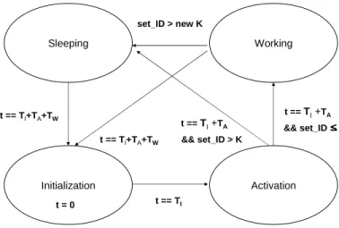
A node with its LID between 1 and K works as a working node during the WP. All the other nodes go to sleep during the WP in the current round. During the WP, if a request for a newK that is less than the currentK is received, each working node compares the newK with its LID and goes to the sleeping state instantly if its LID is greater than the new K, as shown in Fig. 3, which is the state transition diagram for each node during one round. This is another benefit of our protocol for dynamic reconfiguration. If the new K is larger than the current K, reconfiguration occurs in the next round. In Fig. 3, a transition occurs when the local timer (t) of a node indicates the start of the next phase and/or a certain condition is met.

(26)

Sleeping Working Activation t == TI+TA+TW && set_ID K t == TI+TA && set_ID > K set_ID > new K Initialization t == TI t = 0 t == TI+TA+TW t == TI+TA

Fig. 3. State Transition Diagram for Each Node During One Round C. Experimental Results

In this section, we show the results on coverage and network performance with the ROAL protocol.

1. Coverage Evaluation

To measure the coverage, the entire sensing region is divided into 1m × 1m grids. Each point is considered to be covered if the point is located within the sensing range of a working node. The sensing range is 10m, while the communication range is 30m. Fig. 4 (a) and (b) show that the percentages of the covered areas for 1- and 3-coverage networks with the ROAL protocol, respectively. Each bar represents the ratios of resulting coverages for a specific region size/number of nodes. The upper row of the X-axis indicates the size of the region where sensor nodes are deployed. For example, 50 implies a 50m _×50m region. The lower row of the X-axis indicates the number of sensor nodes deployed in the region. The ratio of the uncovered area with 1-coverage in Fig. 4 (a) reaches up to 24% when the density is 0.01 (100 nodes/10,000m2_{), which} is the worst case. If the density exceeds 0.025 (250 nodes/10,000m2_{), the ratio of}

(27)

0% 20% 40% 60% 80% 100% 5 0 6 0 7 0 8 0 9 0 1 0 0 5 0 6 0 7 0 8 0 9 0 1 0 0 5 0 6 0 7 0 8 0 9 0 1 0 0 5 0 6 0 7 0 8 0 9 0 1 0 0 5 0 6 0 7 0 8 0 9 0 1 0 0 100 250 400 550 1000

Region Size / Number of Nodes

C o v e re d A re a 0 1 2 3 4 5

(a) ROAL Protocol with 1-coverage

0% 20% 40% 60% 80% 100% 5 0 6 0 7 0 8 0 9 0 1 0 0 5 0 6 0 7 0 8 0 9 0 1 0 0 5 0 6 0 7 0 8 0 9 0 1 0 0 5 0 6 0 7 0 8 0 9 0 1 0 0 5 0 6 0 7 0 8 0 9 0 1 0 0 100 250 400 550 1000

Region Size / Number of Nodes

C o v e re d A re a 0 1 2 3 4 5 6 7 8 9 10

(b) ROAL Protocol with 3-coverage Fig. 4. Ratios of Covered Areas

(28)

the uncovered area decreases to below 5%. The ratio of the uncovered area with 3-coverage (0-, 1-, and 2-3-coverages) in Fig. 4 (b) reaches up to 50% when the density is 0.01. However, as the density increases, this ratio also becomes small. According to our observation, there still exists around 8% (for 1-coverage) and 23% (for 3-coverage) uncovered area with all sensor nodes working with the same number of nodes and the network size. Hence, the uncovered area incurred by the ROAL protocol is very small, less than 2% of the total region.

Fig. 5 (a) and (b) show the average degrees of 1- and 3-coverage networks with the ROAL protocol. The average degrees of 1-coverage range from 1.1 to 2 with different densities. This implies that the ROAL protocol can efficiently manage the quality of the required degree of coverage using a reasonable number of working nodes. The average degrees of the 3-coverage network also range from 2.5 to 6. Fig. 6 shows the number of working nodes with the region size of 50m_×50m for 1-coverage and 3-coverage, respectively. The actual number of working nodes grows very slowly, while the number of the sensor nodes increases steeply. Compared to the results obtained using the geographic information in the CCP [11], the ROAL protocol can provide very competitive results without using any geographic information. The results on the average degree for 1-coverage and the number of working nodes for 1 and 3-coverage are close to each other. Moreover, since the ROAL protocol requires much lower running overhead compared to the approaches that use the geographic information, it really improves the energy performance of the sensor network. In addition, our protocol can support the desired degree of coverage, which is not provided in PEAS protocol.

(29)

100 200 300 400 500 600 700 800 900 1000 Number of Nodes 50 60 70 80 90 100 Region Size 1.1 1.2 1.3 1.4 1.5 1.6 1.7 1.8 1.9 2 Average Coverage

(a) Average Coverage Degrees with 1-coverage

100 200 300 400 500 600 700 800 900 1000 Number of Nodes 50 60 70 80 90 100 Region Size 2.5 3 3.5 4 4.5 5 5.5 6 Average Coverage

(b) Average Coverage Degrees with 3-coverage Fig. 5. Average Coverage Degree

(30)

! #"%$&(')$*&,+ -. / 012 3 4 56 7 89 1 -3 :1; <=> *?@BADC E => ?@FAC

(a) Number of Working Nodes Fig. 6. Number of Working Nodes

(31)

0 10 20 30 40 50 60 70 80 90 100 0 500 1000 1500 2000 2500 3000

Average Residual Energy (J)

Time (sec)

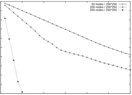
50 nodes / 250*250 200 nodes / 250*250 250 nodes / 250*250

Fig. 7. Average Residual Energy with DSR Only 2. Network Performance

In this section, we evaluate the coverage lifetime and the packet delivery ratio, along with the residual energy of the network using the ns-2 simulator. We use the DSR routing protocol [17] to evaluate the ROAL protocol because it provides an on-demand source routing that does not need any location information and it is the basic routing scheme for other on-demand routing protocols.

For this simulation, 30m is set for the sensing radius and 75m for the communi-cation radius of each node. We use 250m×250m 2-dimensional square for a target sensing region. In addition, there are 10 event points distributed randomly around the upper bound of the sensing area and each point generates 5 events per second. When working nodes around the event points sense the generated events, they send a 512 byte packet per one event to the sink node that is located at the right bottom of the sensing region. The average coverage is measured by counting the number of

(32)

neighboring nodes that detect the event. All results shown in this section are obtained using 1,000 second round time (5 seconds for TI and TA each, and 990 seconds for TW), and simulation data are collected every 100 seconds. Also, each sensor node is given 100 Jules of initial energy.

Fig. 7 shows the average residual energy with the DSR protocol only (i.e., all nodes are working) for 50 nodes, 200 nodes, and 250 nodes, respectively. It is clear that, without any energy-saving scheme, the network with a small number of nodes has more residual energy than the one with a larger number of nodes. This implies that excessively redundant nodes cause more energy consumption with the DSR rout-ing protocol that uses a broadcastrout-ing scheme. Fig. 8 (a) and (b) show the average residual energy and the minimum residual energy of the network for different cover-age degrees (K = 1 and 2). With the ROAL protocol, the network can reserve more energy than with only the DSR protocol.

The average packet delivery ratio is shown in Fig. 9 (a). More than 95% of packets are dropped after 800 seconds with the DSR only. With the ROAL protocol, almost 100% packets are delivered up to 2,900 seconds whenK is 2, and up to 3,000 seconds when K is 1. When K is 2, the delivery ratio drops to 0 after 2,900 seconds because some intermediate nodes between the sources and the sink node completely depletes their energy. Some temporal drops are caused by packet losses during the reconfiguration period. In Fig. 9 (b), the average degree of coverage is shown with 380 sensor nodes. The average degree of 2-coverage remains around 2.0, while 1-coverage shows the average degree over 1 during the whole simulation time. Without the ROAL protocol, the average degree of coverage is around 5 at the beginning of the simulation, but it rapidly drops to around 1 after 300 seconds, since sensor nodes around the event points have died together for energy depletion except about one working node. Therefore, the network with the ROAL protocol can capture the

(33)

events for a longer time since it uses a small number of different working nodes in each round. In addition, the results also prove that the ROAL protocol can provide the required degree of coverage efficiently.

D. Conclusion

In this chapter, we proposed a fast and efficient K-coverage algorithm, called the ROAL protocol, to solve the problem of providing a certain degree of coverage in WSNs. The main idea of the ROAL protocol is to ensure K-coverage usingK subsets of working nodes using the layering concept, where each subset guarantees 1-coverage. The ROAL protocol efficiently constructsK-coverage network with low message over-heads and guaranteed packet delivery with the advantages of energy-savings in the network. Simulation results also support our claim.

In future work, we will suggest more useful schemes to select the working node sets regarding energy burdens in each node and may study on the measurement scheme for the duration of each phase regarding both maximal and a given desired network lifetime. Also, a proper reaction for the event of faulty nodes is an important issue for further study.

(34)

0 20 40 60 80 100 120 0 500 1000 1500 2000 2500 3000 Time (sec) A v e ra g e R e s id u a l E n e rg y ( J ) DSR only DSR+ROAL, K=1 DSR+ROAL, K=2

(a) Average Residual Energy

0 10 20 30 40 50 60 70 80 90 100 200 300 400 500 600 700 800 Time (sec) M in im u m R e s id u a l E n e rg y ( J ) DSR only DSR+ROAL, K=1 DSR+ROAL, K=2

(b) Minimum Residual Energy

(35)

0 0.2 0.4 0.6 0.8 1 1.2 100 600 1100 1600 2100 2600 Time (sec) P a c k e t D e liv e ry R a ti o DSR only DSR+ROAL, K=1 DSR+ROAL, K=2

(a) Packet Delivery Ratio

0 1 2 3 4 5 6 100 600 1100 1600 2100 2600 Time (sec) A v e ra g e C o v e ra g e D e g re e DSR only DSR+ROAL, K=1 DSR+ROAL, K=2

(b) Average Coverage Degree

(36)

CHAPTER III

C-ROAL: CIRCULATION-ROAL ENHANCED WITH FAULT-TOLERANCE FORK-COVERAGE

We previously proposed a randomly ordered activation and layering (ROAL) protocol [18] for K-coverage. Although the K-coverage almost surely can be achieved by the ROAL protocol in a small constant time without the help of the GPS or a virtual coordinate algorithm, it requires a periodic reconfiguration for a fault tolerance and energy balance. In this chapter, we propose a C-ROAL protocol using a new circu-lation scheme to reconfigure the set of working nodes in an autonomous way, where the reconfiguration can be performed with a small and almost constant energy con-sumption. We also provide the model of the expected coverage and connectivity for the layer coverage and show a proper range in which only one node can be activated with regard to a node density and the sensing radius of a node.

The experimental results on the energy consumption show that the fraction of total reconfiguration energy becomes less than 1% of the energy consumed in the ROAL protocol with a high frequency of reconfiguration. Also, we obtain a greatly reduced packet latency, which corresponds to only 5% of the delay that occurred in the ROAL protocol.

The rest of this chapter is organized as follows. The problem related to the fault tolerance of previous studies is discussed in Section A. In Section B, we provide the details of a new C-ROAL protocol. We discuss the analytical model of coverage and connectivity, and show our experimental results on the performance of circulation in Section C. We conclude our work in Section D.

(37)

In the PEAS protocol [10], where a probing scheme selects one node per unit probing area, the probing rate of each sleeping node is adjusted to the desired probing rate specified by the application to keep the rate under the existence of any faulty nodes. Since the frequency of wake-up will increase as the probing rate decreases, the energy overhead for the fault-tolerance becomes high according to the fault rate and the number of deployed nodes. Another problem in PEAS may occur in unbalanced energy burdens. Each node is only deactivated when it depletes all residual energy, which in turn can cause a locally uncovered region.

The CCP protocol is a deterministic approach and has a high time complexity ofO(N3_{), where} _N _{is the number of neighboring nodes. In CCP, each working node} sends a periodic beacon message, while each sleeping node wakes up periodically to hear the beacon messages. The expected overhead of energy for fault-tolerance will also increase as the number of deployed nodes increases.

Set K-Cover problem1 _{[19, 15], which is a probabilistic approach, makes} _K sub-sets using all deployed nodes such that the frequency of covering any point in the interesting area is maximized as many as at least K times, while each subset is ac-tivated in a round-robin fashion. This approach introduced a round-robin coverage that is able to balance the energy consumption with a fault-tolerance. Our circulation method suggested in this study uses the same concept with the round-robin approach. However, our protocol can guarantee K-coverage while circulating one layer at each round.

In our previous study [18], we suggested a randomly ordered activation and layer-1_{Circulation suggested in this study uses the same round-robin approach. However,} our scheme builds as many layers as possible and activates only K layers at a time.

(38)

ing (ROAL) protocol, which provides theK-coverage using a new layering scheme. We proved that the layer coverage makes it simple to build and maintain theK-coverage. However, the accumulative energy consumption spent for a periodic reconfiguration will increase in proportion to the fault rate or the number of deployed nodes.

In this work, we propose a new protocol that can improve the performance of fault-tolerance and energy-balance forK-coverage based on our layer coverage. With our proposed circulation method, we recursively activate a different set of nodes for the fault-tolerance and the energy-balance among all deployed nodes without the repetitive layering procedure of the ROAL protocol. Also, we present the analytical model of the coverage and the connectivity of our layer coverage to verify the effect of the unit size of layering radius to the resultant coverage and connectivity.

B. Circulation-ROAL Protocol

In Chapter II, we introduced a primitive reconfiguration scheme where all nodes wake up and generate a random and uniformly distributed activation time Ta. When its Ta expires, a node looks up any available layer that has not yet been selected by its neighbors, and will be activated by sending an ACTIVE message if one of K layers is missing. Since the ROAL protocol repeats the layering procedure at every working period, the potential cost of energy will be increased as the frequency of layering is raised for an increased fault ratio. The reason is because the ROA algorithm needs to buildK layers at every round. We resolve this problem by modifying the layering procedure such that all possible layers are built at the first period and we circulate them at every period, removing the repetitive layering procedure.

(39)

1. Model of Circulation-ROAL (C-ROAL)

In this section, we explain the details on the C-ROAL protocol that circulates the layers without repeating the layering procedure at every working round Tw as the ROAL protocol needs. First, we define by L(l) a set of nodes that have a layer ID (LID) l.

Algorithm C-ROA (K, TA)

1. t_←0 2. LID_←0 3. H _{← ∅} 4. Ta ←rand(0, TA) 5. while t < TA 6. ift =Ta

7. LID_← minl_|H(l) =f alse

8. send ACTIVE.LID

9. else if ACTIVE.LID arrives 10. H(LID)←true

11. ifh←max[H] is less than or equal to K

12. Tw =_∞

(40)

14. calculate Tw and go to work 15. else

16. calculate Ts and go to sleep

Every node obtains its LIDl when itsTa expires. In the original ROAL protocol, only K layers are formed by the ROA algorithm. However, the C-ROA algorithm assigns layer id to all nodes. Then, each node will act following the circulation rule either setting a sleeping period (Ts) or a working period (Tw) based on its LID. The calculation of Tw and Ts is explained in the next section. Based on its LID, every node calculates its working or sleeping period.

2. Circulation Rule

A circulation rule is developed for the purpose of a low-power reconfiguration of work-ing nodes while providwork-ing a robust and energy-balancedK-coverage. Usually, a sleep-ing node needs to wake up with a certain frequency to monitor if some healthy nodes are working within its sensing range for assuring a reliable quality of K-coverage. Hence, the frequency of the fault detection messages will be increased as a fault ratio increases, which deteriorates the energy credit in WSNs. A different way is implemented in this study using the circulation scheme that substitutes a set of working nodes with a different set of sleeping nodes, meanwhile guaranteeing a con-stant K-coverage. This property differentiates our approach from the Set K-cover study in that the degree of coverage can be changed whenever a different set is acti-vated [19, 15].

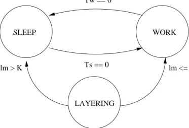
Fig. 10 shows the state transition diagram of circulation. Using a LID obtained by the C-ROA algorithm, each node calculates Tw or Ts. Whenever Tw of working nodes orTs of sleeping nodes expires, each node transits its state, as shown in Fig. 10.

(41)

Hence, the transition between the working and sleeping state happens autonomously, which can reduce the energy consumed for a repetitive layering at every round as in the ROAL protocol.

lm > K lm <= K LAYERING Ts == 0 Tw == 0 WORK SLEEP

Fig. 10. State Transition with Circulation

We implement a deterministic circulation, which uses a fixed and constant recon-figuration time Tr. Each node calculates its Ts or Tw using the predefined Tr. Each node knows the highest LIDh by hearing the packets exchanged during the layering procedure. With a given degree of coverage K, its LID l, the highest layer id h and Tr, a node determines both Ts and Tw as follows.

A. Initial calculation forTw and Ts

Initially, we need to activate all K layers for the first round. Each node that has a LID_≤K decides to work and calculates its Tw. Tw will be different according to its LID l since only nodes in the bottom layer, i.e., layer 1, will sleep after this first round. For this reason, nodes that have LIDl less than or equal to K will work duringTw that is calculated by:

(42)

Tw(l) =      Tr_×l, if l_≤K and h > K ∞, if l _≤K and h_≤K.

If the highest LID h of a node v is smaller than K, v will set its Tw =∞. If its LID is greater thanK, v will go to sleep during Ts calculated as follows:

Ts(l) = (l₋K)_×Tr, if l_≥K.

We circulate one layer in a sequence ofC(1), C(2), C(3), . . . , C(h) at every Tr, while sustainingK layers at every time instance. The term of circulationC(l) defines that working nodes in layer l go to sleep and sleeping nodes in layer m wake up to work, where m= (K+l) mod h, if m >0, or m =h if not.

B. After initial calculation

Once the first period of working or sleeping mode finishes, the way of calculation changes as follows.

Tw(l) =Tr×K Ts(l) = (h−K)×Tr.

Note that a current working node will have a newTs and a newly wake-up node will calculate a new Tw. Because each node can decide its Tw andTs using h and its LID with the given values ofTr andK, a local difference of density will not affect the the overall coverage.

(43)

3. Discussion on Fault Tolerance

Using the circulation scheme, we can provide an energy efficient fault tolerance while maintaining K-coverage. First of all, the K-coverage itself is a scheme to provide a high probability of detection unless K nodes within the unit sensing area have fault. In addition, the circulation scheme can provide a more robust environment by circulating a faulty layer with a new healthy layer. If we can decrease the interval of circulation, the recovery time for the faulty region can be minimized. We concern the cost of reconfiguration in terms of both the energy efficiency and the network performance. As shown in the experiment of an energy and delay in Section 3, the circulation proves itself as an energy-efficient fault-tolerant scheme for K-coverage in that the energy consumed for the reconfiguration remains almost constant and small even if the frequency of the reconfiguration increases dramatically. As well as the fault-tolerance, the circulation scheme is a good method for the energy-balance because a set of nodes belonging to a layer will be activated in a round-robin fashion. For the summary, we can say that the C-ROAL protocol provides a robust and energy-efficient fault-tolerance with energy-balance.

C. Analysis on Layer Coverage

In this section, we analyze the probability of the coverage and connectivity of our layer coverage. The coverage and connectivity depends on the layering radius of rl, the sensing radius ofrs, the communication range rc, and a node density. We assume that the positions of nodes follow the Poisson point process of constant and finite density λ in area R2. Here, we assume that there will be no collision during the layering procedure for the simplicity of proof.

(44)

πr2 _{centered at a random point follows the Poisson distribution such as} _P_{(i, r) =} e−λπr2

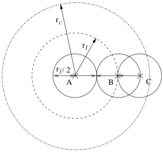
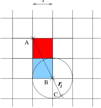
(λπr2₎i_{/i!. At a random position, each node decides its layer by running ROA} or C-ROA algorithm. Assume that the layering radius is rl where a node sends an ACTIVE message to its neighbors. As shown in Fig. 11, the minimum distance between any nodes in the same layer will be rl/2, and there is only one node within the area of π(rl/2)2 as depicted with the smallest ball in Fig. 11.

C A B / 2 l r c r l r

Fig. 11. Minimum Distance between Two Working Nodes

1. Connectivity

The connectivity will be guaranteed in our layer coverage if any on-duty node working for a certain layer is connected. We mean by connected that any two nodes can reach to each other in multiple hops. We follow a similar procedure, as shown in the study [20] to prove the connectivity, but provide a different model using the Poisson point process model.

(45)

Poisson point process model, Then, there is almost surely at least 1 node per unit area of d2 _when_l _{goes to infinity if the density of nodes satisfies} _λ₌ klnl2

d2 fork > 1.

Proof. We divide the region _RintoN = l2

d2 squares of sized×d. Letµ0(n, N) be the random variable denoting the number of empty squares of size d_×d, where n is the number of nodes in area R, and p0 is the probability of empty nodes in one square. Then, the expected number of empty cellE[µ0(n, N)] will be:

E[µ0(n, N)] =N _·p0 =N _·e−λd2

=N e−nN−1

.

Here, we want to findE[µ0(n, N)] when l _{→ ∞}. From the above equation, we obtain: lnE[µ0(n, N)] = ln l2

d2 − nd 2

l2 .

If we assumend2 ₌_kl2_ln_l2_{, the above equation becomes:} lnE[µ0(n, N)] = ln 1

d2_l2k−2.

Ifk >1, then

limn,N→∞lnE[µ0(n, N)] = −∞.

Hence, limn,N→∞E[µ0(n, N)] = 0 and there almost surely is at least 1 node in each

square. The density of nodes will be: λ= _ln2 =

klnl2

d2 , where k >1.

The connectivity will be satisfied if the communication range is greater than or equal to the expected maximum distance between two working nodes as proved in Theorem 1.

Theorem 1. A maximum distance between two active nodes that belong to the same layer is less than or equal to (1 +√5)_×rl if the density of nodes is satisfied as in Lemma 1.

(46)

Proof. Based on the condition of density derived in Lemma 1, we follow the complete proof of Lemma 3.1 and Theorem 3.1 in [10]. We assume that each square in Fig. 11 has only one node considering the worst case of Lemma 1 where d = rl. Because there will be only one node per each square, node B is the furtherest node to be activated away from A in the gray square if A is activated in the dark square as shown in Fig. 12. However, if node C is activated earlier than B within the layering radius of rl from B, node B will sleep. The distance between node A and node C is the maximum distance where any two working nodes can be apart from each other. Hence, the communication range rc = (1 +√5)rl is a minimum range to guarantee the connectivity. The details can be found in [10].

In addition, the connectivity for one layer of Theorem 1 is a sufficient condition for the case of K-coverage.

r

_l l

r

B

C

A

(47)

2. Coverage

If a given sensor network has the density λ, we can scale down the density to λl(1) for 1-coverage obtained by the ROA or ROA algorithm. Because ROA and C-ROA selects one node per area of π(rl/2)2_{, the scaled-down density will be} _{λl(1) =}

1

π(rl/2)2λ =

4λ πr2

l. According to the Poisson point process model, the coverage is the

probability of empty node within the sensing radius of rs. Hence, the percentage of 1-coverage will be:

Rc = 1−e−λl(1)πr2s

= 1₋e−4λα−2, α=rl/rs.

(3.1)

From (3.1), a minimum required density for Rc almost surely is calculated by λ = −ln(1−Rc)

4 ·(

rl rs)

2_. _(3.2)

ForK-coverage, one can easily calculate a required density by λl(K) = _π(rK_l_/2)2 ·λ.

3. Simulation

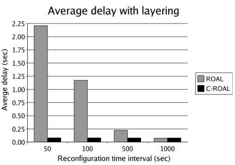
Using 300 nodes deployed over a two-dimensional area of 500m_×500m, we obtain the total energy consumed for the layering procedure and the average delay incurred for data packet delivery using the ns-2 simulator. The other options are 25m forrs, 70m for rc, and K = 3. Dynamic source routing (DSR) is used as a routing protocol. In Fig. 13, we compare the energy consumption for the reconfiguration. The C-ROAL protocol consumes a constant small energy for the layering procedure even though the reconfiguration periods vary from 50 to 1,000 seconds. However, the total energy consumption increases greatly as the reconfiguration period becomes shorter in the ROAL protocol. We also show the average delay of a data packet incurred by the

(48)

reconfiguration in Fig. 14. We can see that the packets are delivered much faster with the C-ROAL protocol, while the delay is increasing as the number of reconfiguration is increased in ROAL. The reason is because C-ROAL protocol never deters the packet delivery due to the autonomous circulation. We also expect that the difference of the total reconfiguration energy will be increased as the number of nodes increases. From the above results, we can say that the C-ROAL protocol can greatly improve the energy efficiency, while providing K-coverage with both the energy-balance and the fault-tolerance together for WSNs.

Fig. 13. Comparison of Energy Consumption for Reconfiguration

D. Conclusion

In this chapter, we developed the C-ROAL protocol that can improve the fault-tolerance and energy-balance for K-coverage using a new circulation and C-ROA

(49)

Fig. 14. Average Delay Incurred by Reconfiguration

scheme. We also proved that the C-ROAL protocol can guarantee the connectivity and coverage if a certain minimum density is satisfied regarding the sensing and the layering radius. The C-ROAL protocol can reconfigure the sets of working nodes with a greatly decreased energy consumption compared to the ROAL protocol. This property enhances the energy balance and fault tolerance for WSNs.

In future work, we will implement a more concrete strategy that can replace a fault node in a certain layer with a healthy node in other layers to stabilize the QoS during the network lifetime.

(50)

CHAPTER IV

MRCC: MOBILITY RESILIENT COVERAGE CONTROL FOR K-COVERAGE In this chapter, we consider more realistic WSN environments where the sensor nodes are moving around, which can disappear due to wear-out failures. By enhancing a variant of the Random WayPoint (RWP) model [21], we propose Mobility Resilient Coverage Control (MRCC) to assure K-coverage in the presence of mobility. Our basic goals are 1) to elaborate the probability of breaking K-coverage with moving-in and movmoving-ing-out probabilities, and 2) to issue wake-up calls to sleepmoving-ing sensors to meet user requirement ofK-coverage even in the presence of mobility. Furthermore, to show the impact of wear-out failures on the coverage achieved, we adopt a lognormal distribution to depict the conditional probability of failures and observe the influence of reduced numbers of active nodes on coverage. Our experiments with ns-2 show that MRCC achieves better coverage by 1.4% with 22% fewer active sensors than that of the existing Coverage Configuration Protocol (CCP). By taking the reliability of nodes into account, the performance drop with respect to coverage is 3.7% (for coverage > 1), while the reduction in the number of sensor nodes is 18.19% when compared with pure MRCC. Comparing CCP and MRCC with reliability, we observe a 3.4% reduction in coverage for the average probabilistic case and 5.78% for the individual probabilistic case, while achieving a 12.82% and 28.2% reduction in number of nodes, respectively.

The rest of this chapter is organized as follows. Section A discusses the exist-ing works and Section B introduces the basic concept and corollaries ofK-coverage. In addition, we reformulate the average and individual probabilities in the mobil-ity model. We will explain the experiments conducted with NS2 for our scheme in Section C. Finally, the conclusion and future work are mentioned in Section D.

(51)

There are many obstacles to induce a fault in guaranteeing the coverage in real WSN environments. As an undermining factor ofK-coverage requirement, we would like to focus on mobile sensor nodes with wear-out failures. Mobility with wear-out failures in a WSN are one of the sources that make solutions of the above problems harder [21, 22] and the same is true for Ad Hoc networks [23, 24, 25]. In solving the problem of mobility with failures, the biggest concern is that of maintaining a connected and covered network, while minimizing the power consumption so that the sensed data are safely delivered even in the presence of breaking the confidence of coverage and connectivity.

Span [26] was designed to adaptively elect coordinators among all the nodes in the network. Its goals are to ensure that sufficient coordinators are elected so that every node is within the radio range of at least one coordinator and to rotate the coordinators through the withdrawal mechanism in order to ensure that all nodes share the task of providing global connectivity. Based on Span, Coverage Control Protocol (CCP) [11] was devised to provide a specific coverage degree requested by an application with a decentralized protocol that only depends on local states of sensing neighbors. In contrast to stationary WSNs stated above, we consider mobility in guaranteeingK-coverage.

To properly model the mobility of a sensor or a vehicle, [27] suggested a scheme where mobile objects are uniformly distributed over a cell. Each sensor chooses a direction θ and speed v, uniformly at random in intervals [0,2π) and [0,Vmax] respec-tively. With the optional operation ofthinking time, the Random WayPoint (RWP) model similar to [27] has been a commonly used synthetic model for mobility in Mobile Ad hoc Networks (MANETS) [25, 28]. However, this model fails to provide a steady

(52)

state in that the average nodal speed consistently decreases over time, and therefore should not be directly used for simulation. So [29] suggested a modified Random WayPoint model to be able to reach a steady state. For the coverage problem, [22] chose a directionθ _∈[0,2π) and a speedv _∈[0,Vmax] according to distribution density functions, fθ(θ) andfV(v), respectively. A mobility model was used by [21] for choos-ing a WayPoint uniformly like RWP to build a robust connectivity topology-Minimum Spanning Tree. The approach of [22] is that a sensor sweeping a field can give better coverage. The difference between [22] and ours is that [22] considered sweeping an area with lack of sensors, while our scheme guarantees K-coverage all the time even if some sensors leave their duty area. In [30], authors suggested several algorithms that identify and minimize existing coverage holes based on Voronoi diagram and then compute the desired target positions where sensors capable of movement should move, while sensors in our scheme are unable to specify their destinations.

Certain work that has been proposed in literature with respect to mobility of nodes can be found in [31]. Here, Random Walk, Random WayPoint, Random Di-rection, Gauss-Markov, and Probabilistic Random Walk have been explained in rea-sonable detail, while [32] deals mainly with achieving steady state of movement with the help of a Random WayPoint model. [21, 22] suggest improvement in coverage achieved with mobility, and we further reinforce this argument with the help of the-oretical formulations as well as simulations, by showing the same in the presence of both mobility and reliability considerations.

B. Mobility Model and MRCC Protocol

Based on the general K-coverage used in the previous chapter, we want to state some corollaries giving the surplus number of sensors to assure the degree of coverage by

(53)

issuing wake-up calls to sleeping sensors for this work.

Corollary 1 _{If a given topology of a WSN is assured by an optimal algorithm for}

K-coverage regardless of the distribution of a set of sensors, the active sensor node has to keep at leastK₋1neighbors in its sensing rangeRs because the point of active sensor needs to be covered byK ₋1 neighbors and itself.

Corollary 2 _{In a given topology assured by an optimal algorithm for} _K_-coverage,

when a sleeping sensor initiates its sensing activity within its sensing range, it should have at least K neighbors on already active duty in its sensing range by the definition of K-coverage.

Based on the sufficient condition ofK-coverage expressed in these corollaries, we plan to devise a mobility-resilient topology control with a modified Random Way-Point model for mobility in the following sections. To enforce the requirement of K-coverage, the above corollaries specify the number of active sensors required to prevent frailty of K-coverage.

1. Probabilities in Mobility Model

Like RWP [25], but unlike the Brownian- or RWP-like mobility model in [21], we consider two probabilities of sensors moving-in/out, as average and individual. Fur-thermore, we reformulate the moving-in probability with the location area Ad of outside sensors which deemed to move in while [21] used A0 in the conditional part. We compare the difference in calculating the moving-in probability with [21] and de-rive the average and individual probabilities with the following assumption of our mobility model; 1) All nodes are randomly distributed within a circle of area A0 with sensing radiusR and the total number of nodesN is known, 2) for a short-term interval of length t, each node moves independently toward a random direction in

(54)

Ad

a

R r

b x

sensor a’s sensing area

moving area sensor b’s max c C(a,R) 1 A (a) Moving In

A

₂

A

0

a

R

x

c

r

b

(b) Moving Out Fig. 15. Probability of Moving In vs. Moving Out

[0,2π), with a constant speed v that is uniformly distributed in [0, vmax] and it may stay still for a while, and 3) the locations of sensors are known using an expensive GPS or a cheap method of trilateration.

Under these assumptions, within a range interval r, which is a function of time t, we can calculate two probabilities 1) that a new neighbor sensor b moves into the detection range of nodeain Fig. 15 (a), and 2) that an existing neighbor bmoves out of the detection range C(a, R) in Fig. 15 (b), Pm.i and Pm.o, respectively. C(a, R) is denoted as the circle of radius R centered at point a of node (a.k.a. point) a.

a. Probability of Moving In C(a, R), Pm.i

Suppose nodeais located at pointawith its neighborbat pointb, as shown in Fig. 15 (a). The maximum detection range of node a is R and the distance between node a and b isx, where x is equal to or larger than R. Also, let point c be an intersection of a circle made by pointa with radiusR and a circle made by maximum movement of point b with velocity vmax and time t. Then bc becomes r = vmax _·t and the

(55)

probability that nodeb moves into the detection range of nodea within timet is the probability that node b moves into the circle C(a, R), which is exactly the shaded area between two circles as shown in Fig. 15 (a). This probability can be calculated in terms of the following two cases.

Case I:₀_{< r <}_2R Pm.i= Z R+r R 2πx Ad A1 πr2dx= Z R+r R 2A1x Adr2 dx, (4.1)

where A1 =α1R2+α2r2−xRsinα1, Ad =π((R+r)2−R2) =π(2rR+r2), α1=∠cab=

arccosx2+R_2xR2−r2, andα2 =∠cba= arccosx

2_+r2₋_R2 2xr . Case II: _r_≥_2R Pm.i= Z r−R R 2πx Ad πR2 πr2 dx+ Z r+R r−R 2πx Ad A1 πr2dx = Z r−R R 2πR2x Adr2 dx+ Z r+R r−R 2A1x Adr2 dx =R 2_(r₋_2R) r2_(r_{+ 2R)} + Z r+R r−R 2A1x Adr2 dx. (4.2)

The first fraction in (4.1) explains the conditional probability about the existence of a sensor at point x and the second fraction is the ratio of areaA1 to total area of nodeb’s movement. Unlike [21] in (4.1) and (4.2), we considered Ad as a conditional probability because the probability of location of outside sensors is represented by

Ad, not A0. The first term of (4.2) considers the case that the movement circle is larger than the circle of sensor a so that the former circle includes the latter. The second term in (4.2) represents a situation where there is an intersection between the movement circle and the sensing circle of sensor a.

(56)

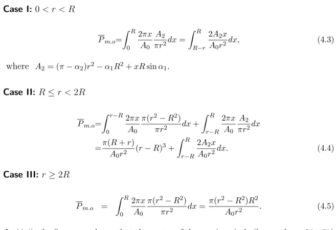
b. Probability of Moving Out C(a, R), Pm.o

The probability that one of the neighbors C(b, R) moves out of the detection range of node a within time t is the probability that node b moves out of circle C(a, R), more specifically, which is the shadowed area outside of the detection circle made by nodea, as shown in Fig. 15 (b). There are three possibilities because the range of the node either 1) intersects, 2) includes, or 3) intersects and includes the given node in the following manner,

Case I:₀_{< r < R} Pm.o= Z R 0 2πx A0 A2 πr2dx= Z R R−r 2A2x A0r2 dx, (4.3) where A2 = (π−α2)r2−α1R2+xRsinα1. Case II: _R_≤_{r <}_2R Pm.o= Z r−R 0 2πx A0 π(r2−R2) πr2 dx+ Z R r−R 2πx A0 A2 πr2dx =π(R+r) A0r2 (r₋R)3+ Z R r−R 2A2x A0r2 dx. (4.4) Case III:_r_≥_2R Pm.o = Z R 0 2πx A0 π(r2₋R2) πr2 dx= π(r2₋R2)R2 A0r2 . (4.5)

In (4.4), the first term shows that the center of the moving circle (larger than C(a, R)) ranges from 0 tor−Rresulting in the moving circle encompassing the circle C(a, R), while the second term accounts for the intersection between the moving circle and circle C(a, R).

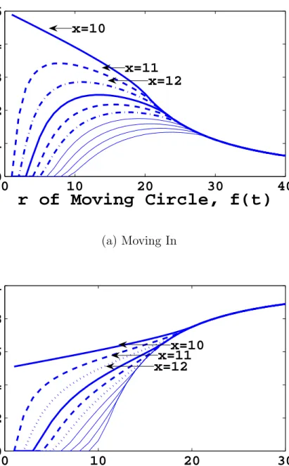
Fig. 16 depicts the functions, Pm.iand Pm.o, considering (4.1) to (4.5) according torforRs = 10 whose value decides the stiffness of these functions, not the monotonic

(57)

0

10

20

30

0

0.2

0.4

0.6

0.8

1

r of Moving Circle, f(t)

Probability

Avg. Probability of In/Out

Moving In

Moving Out

Fig. 16. Pm.i vs. Pm.o

increase or decrease. While Pm.i starts at 0.2 and decreases gradually, Pm.oincreases expeditiously. (4.1) through (4.5) have been devised for average probability, meaning that regardless of the distance given by variable X, from the area of interest, every sensor has the same probability. But, intuitively, at given time t, sensors outside or inside the rim have a larger probability of moving in or out, respectively. Therefore, if we specify this individual probability of moving in and out, each sensor can make a more accurate decision. This insight can be formalized in the following equations,

Pm.i|X=x=              A1 πr2 0< r <2R, R≤x < R+r R2 r2 r≥2R, R≤x < r−R A1 πr2 r≥2R, r−R≤x≤r+R (4.6)