Model based Word Embeddings from Decompositions of Count Matrices

Model-based Word Embeddings from Decompositions of Count Matrices

Karl Stratos Michael Collins Daniel Hsu

Columbia University, New York, NY 10027, USA {stratos, mcollins, djhsu}@cs.columbia.edu

Abstract

This work develops a new statistical un-derstanding of word embeddings induced from transformed count data. Using the class of hidden Markov models (HMMs) underlying Brown clustering as a genera-tive model, we demonstrate how canoni-cal correlation analysis (CCA) and certain count transformations permit efficient and effective recovery of model parameters with lexical semantics. We further show in experiments that these techniques empir-ically outperform existing spectral meth-ods on word similarity and analogy tasks, and are also competitive with other pop-ular methods such as WORD2VEC and GLOVE.

1 Introduction

The recent spike of interest in dense, low-dimensional lexical representations—i.e., word embeddings—is largely due to their ability to cap-ture subtle syntactic and semantic patterns that are useful in a variety of natural language tasks. A successful method for deriving such embed-dings is the negative sampling training of the skip-gram model suggested by Mikolov et al. (2013b) and implemented in the popular software WORD2VEC. The form of its training objective was motivated by efficiency considerations, but has subsequently been interpreted by Levy and Goldberg (2014b) as seeking a low-rank factor-izationof a matrix whose entries are word-context co-occurrence counts, scaled and transformed in a certain way. This observation sheds new light on WORD2VEC, yet also raises several new ques-tions about word embeddings based on decompos-ing count data. What is the right matrix to de-compose? Are there rigorous justifications for the choice of matrix and count transformations?

In this paper, we answer some of these ques-tions by investigating the decomposition specified by CCA (Hotelling, 1936), a powerful technique for inducing generic representations whose com-putation is efficiently and exactly reduced to that of a matrix singular value decomposition (SVD). We build on and strengthen the work of Stratos et al. (2014) which uses CCA for learning the class of HMMs underlying Brown clustering. We show that certain count transformations enhance the ac-curacy of the estimation method and significantly improve the empirical performance of word rep-resentations derived from these model parameters (Table 1).

In addition to providing a rigorous justifica-tion for CCA-based word embeddings, we also supply a general template that encompasses a range of spectral methods (algorithms employing SVD) for inducing word embeddings in the lit-erature, including the method of Levy and Gold-berg (2014b). In experiments, we demonstrate that CCA combined with the square-root transforma-tion achieves the best result among spectral meth-ods and performs competitively with other popu-lar methods such as WORD2VEC and GLOVE on word similarity and analogy tasks. We addition-ally demonstrate that CCA embeddings provide the most competitive improvement when used as features in named-entity recognition (NER). 2 Notation

We use[n]to denote the set of integers{1, . . . , n}. We denote them×mdiagonal matrix with values

v1. . . vm along the diagonal by diag(v1. . . vm). We write [a1. . . am]to denote a matrix whosei -th column isai. The expected value of a random variableXis denoted byE[X]. Given a matrixΩ and an exponenta, we distinguish the entrywise power operationΩhai _{(i.e., Ω}hai

i,j = (Ωi,j)a) from the matrix power operation Ωa _{(defined only for} squareΩ).

3 Background in CCA

In this section, we review the variational charac-terization of CCA. This provides a flexible frame-work for a wide variety of tasks. CCA seeks to maximize a statistical quantity known as the Pear-son correlation coefficient between random vari-ablesL, R∈R:

Cor(L, R) := p E[LR]−E[L]E[R]

E[L2_]−E[L]2p_E[R2_]−E[R]2

This is a value in[−1,1]indicating the degree of linear dependence betweenLandR.

3.1 CCA objective LetX∈Rn_{andY ∈R}n0

be two random vectors. Without loss of generality, we will assume thatX

and Y have zero mean.1 _{Let m ≤ min(n, n}0_).

CCA can be cast as finding a set of projection vec-tors (called canonical directions)a1. . . am ∈ Rn andb1. . . bm ∈Rn0 such that fori= 1. . . m:

(ai, bi) = arg max

a∈Rn_{, b∈R}n0 Cor(a

>_{X, b}>_{Y) (1)}

Cor(a>_{X, a}>

jX) = 0 ∀j < i Cor(b>Y, b>_jY) = 0 ∀j < i

That is, at eachiwe simultaneously optimize vec-tors a, b so that the projected random variables

a>_{X, b}>_{Y ∈Rare maximally correlated, subject}

to the constraint that the projections are uncorre-lated to all previous projections.

Let A := [a1. . . am] and B := [b1. . . bm]. Then we can think of the joint projections

X =A>X Y =B>Y (2)

as newm-dimensional representations of the orig-inal variables that are transformed to be as corre-lated as possible with each other. Furthermore, of-tenmmin(n, n0_{), leading to a dramatic}

reduc-tion in dimensionality.

3.2 Exact solution via SVD

Eq. (1) is non-convex due to the termsaandbthat interact with each other, so it cannot be solved exactly using a standard optimization technique. However, a method based on SVD provides an efficient and exact solution. See Hardoon et al. (2004) for a detailed discussion.

1_{This can be always achieved through data preprocessing} (“centering”).

Lemma 3.1 (Hotelling (1936)). Assume X and

Y have zero mean. The solution (A, B) to (1) is given by A = E[XX>_]−1/2_{U and B =}

E[Y Y>_]−1/2_{V where the i-th column of U ∈} Rn×m _{(V ∈ R}n0_×m

) is the left (right) singular vector of

Ω :=E[XX>_]−1/2_E[XY>_{]E[Y Y}>_]−1/2 ₍₃₎

corresponding to thei-th largest singular valueσi. Furthermore,σi =Cor(a>i X, b>i Y).

3.3 Using CCA for word representations As presented in Section 3.1, CCA is a general framework that operates on a pair of random vari-ables. Adapting CCA specifically to inducing word representations results in a simple recipe for calculating (3).

A natural approach is to set X to represent a word and Y to represent the relevant “context” information about a word. We can use CCA to project X and Y to a low-dimensional space in which they are maximally correlated: see Eq. (2). The projectedXcan be considered as a new word representation.

Denote the set of distinct word types by[n]. We setX, Y ∈ Rn_{to be one-hot encodings of words} and their associated context words. We define a context word to be a word occurring withinρ po-sitions to the left and right (excluding the current word). For example, with ρ = 1, the following snippet of text where the current word is “souls”:

Whatever our souls are made of

will generate two samples of X ×Y: a pair of indicator vectors for “souls” and “our”, and a pair of indicator vectors for “souls” and “are”.

CCA requires performing SVD on the following matrixΩ∈Rn×n_:

Ω =(E[XX>_]−E[X]E[X]>₎−1/2 (E[XY>_]−E[X]E[Y]>₎ (E[Y Y>_]−E[Y]E[Y]>₎−1/2

At a quick glance, this expression looks daunting: we need to perform matrix inversion and multipli-cation on potentially large dense matrices. How-ever, Ω is easily computable with the following observations:

2011). To see why, let{(x(i)_{, y}(i)_)}N

i=1beN sam-ples ofXandY. Consider the sample estimate of the termE[XY>_]−E[X]E[Y]>_:

1

N

N

X

i=1

x(i)_(y(i)₎>₋ 1

N2 N

X

i=1

x(i)

! _N X

i=1

y(i)

!>

The first term dominates the expression whenNis large. This is indeed the setting in this task where the number of samples (word-context pairs in a corpus) easily tends to billions.

Observation 2. The (uncentered) covariance matrices E[XX>_{] and E[Y Y}>_{] are diagonal.}

This follows from our definition of the word and context variables as one-hot encodings since E[XwXw0] = 0forw6=w0 andE[Y_cY_c0] = 0for c6=c0_.

With these observations and the binary definition of (X, Y), each entry in Ω now has a simple closed-form solution:

Ωw,c = pP(Xw= 1, Yc= 1)

P(Xw= 1)P(Yc= 1) (4)

which can be readily estimated from a corpus.

4 Using CCA for parameter estimation In a less well-known interpretation of Eq. (4), CCA is seen as a parameter estimation algorithm for a language model (Stratos et al., 2014). This model is a restricted class of HMMs introduced by Brown et al. (1992), henceforth called the Brown model. In this section, we extend the result of Stratos et al. (2014) and show that its correctness is preserved under certain element-wise data trans-formations.

4.1 Clustering under a Brown model

A Brown model is a 5-tuple (n, m, π, t, o) for

n, m∈Nand functionsπ, t, owhere

• [n]is a set of word types.

• [m]is a set of hidden states.

• π(h)is the probability of generatingh∈[m] in the first position of a sequence.

• t(h0_{|h)is the probability of generatingh}0 _∈ [m]givenh∈[m].

• o(w|h) is the probability of generatingw ∈

[n]givenh∈[m].

Importantly, the model makes the following addi-tional assumption:

Assumption 4.1 (Brown assumption). For each word typew∈ [n], there is a unique hidden state

H(w) ∈ [m] such that o(w|H(w)) > 0 and

o(w|h) = 0for allh6=H(w).

In other words, this model is an HMM in which observation states are partitioned by hidden states. Thus a sequence of N words w1. . . wN ∈ [n]N has probabilityπ(H(w1))×QiN=1o(wi|H(wi))×

Q_N−1

i=1 t(H(wi+1)|H(wi)).

An equivalent definition of a Brown model is given by organizing the parameters in matrix form. Under this definition, a Brown model has param-eters (π, T, O) where π ∈ Rm _{is a vector and}

T ∈ Rm×m_{, O ∈ R}n×m _{are matrices whose} en-tries are set to:

πh =π(h) h∈[m]

Th0_,h=t(h0|h) h, h0 ∈[m] Ow,h =o(w|h) h∈[m], w∈[n] Our main interest is in obtaining some represen-tations of word types that allow us to identify their associated hidden states under the model. For this purpose, representing a word by the correspond-ing row ofO is sufficient. To see this, note that each row of O must have a single nonzero entry by Assumption 4.1. Let v(w) ∈ Rm _{be the w} -th row ofO normalized to have unit2-norm: then

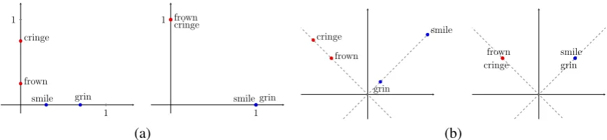
v(w) =v(w0_{)iffH(w) =H(w}0_{). See Figure 1(a)}

for illustration.

A crucial aspect of this representational scheme is that its correctness is invariant to scaling and rotation. In particular, clustering the normalized rows of diag(s)Ohai_diag(s2)Q> _{where O}hai _is

any element-wise power of O with any a 6= 0,

Q∈Rm×m_{is any orthogonal transformation, and}

s1 ∈ Rn and s2 ∈ Rm are any positive vectors yields the correct clusters under the model. See Figure 1(b) for illustration.

4.2 Spectral estimation

1 1

smile grin frown cringe

1 1

smile grin frown

cringe _smile

grin frown cringe

smile grin frown

cringe

(a) (b)

Figure 1: Visualization of the representational scheme under a Brown model with2hidden states. (a) Normalizing the original rows ofO. (b) Normalizing the scaled and rotated rows ofO.

spectral method for consistent parameter estima-tion ofO.

To state the theorem, we define an additional quantity. Letρbe the number of left/right context words to consider in CCA. Let (H1, . . . , HN) ∈ [m]N _{be a random sequence of hidden states} drawn from the Brown model whereN ≥2ρ+ 1. Independently, pick a positionI ∈[ρ+ 1, N −ρ] uniformly at random. Define π˜ ∈ Rm _where ˜

πh :=P(HI=h)for eachh∈[m].

Theorem 4.1. Assume π >˜ 0 and rank(O) = rank(T) = m. Assume that a Brown model (π, T, O) generates a sequence of words. Let

X, Y ∈ Rn _{be one-hot encodings of words and} their associated context words. Let U ∈ Rn×m be the matrix ofmleft singular vectors ofΩhai _∈

Rn×n _{corresponding to nonzero singular values} whereΩis defined in Eq. (4) anda6= 0:

Ωh_w,cai = pP(Xw = 1, Yc= 1)a

P(Xw = 1)aP(Yc= 1)a Then there exists an orthogonal matrix Q ∈

Rm×m _{and a positive s ∈ R}m _{such that U =}

Oha/2i_diag(s)Q>_.

This theorem states that the CCA projection of words in Section 3.3 is the rows ofOup to scaling and rotation even if we raise each element ofΩin Eq. (4) to an arbitrary (nonzero) power. The proof is a variant of the proof in Stratos et al. (2014) and is given in Appendix A.

4.3 Choice of data transformation

Given a corpus, the sample estimate of Ωhai _is

given by:

ˆΩhai

w,c= #(w, c) a

p

#(w)a_#(c)a (5)

where#(w, c)denotes the co-occurrence count of word w and context c in the corpus, #(w) :=

P

c#(w, c), and #(c) := Pw#(w, c). What choice ofais beneficial and why? We usea= 1/2 for the following reason: it stabilizes the variance of the term and thereby gives a more statistically stable solution.

4.3.1 Variance stabilization for word counts The square-root transformation is a variance-stabilizing transformation for Poisson random variables (Bartlett, 1936; Anscombe, 1948). In particular, the square-root of a Poisson variable has variance close to1/4, independent of its mean. Lemma 4.1(Bartlett (1936)). LetXbe a random variable with distribution Poisson(n×p)for any

p ∈ (0,1)and positive integer n. Define Y :=

√

X. Then the variance ofY approaches1/4 as

n→ ∞.

This transformation is relevant for word counts because they can be naturally modeled as Pois-son variables. Indeed, if word counts in a corpus of lengthN are drawn from a multinomial distri-bution over [n] with N observations, then these counts have the same distribution as n indepen-dent Poisson variables (whose rate parameters are related to the multinomial probabilities), condi-tioned on their sum equalingN(Steel, 1953). Em-pirically, the peaky concentration of a Poisson dis-tribution is well-suited for modeling word occur-rences.

4.3.2 Variance-weighted squared-error minimization

At the heart of CCA is computing the SVD of the Ωhai _{matrix: this can be interpreted as solving the}

following (non-convex) squared-error minimiza-tion problem:

min uw,vc∈Rm

X

w,c

Ωhai

w,c−u>wvc

But we note that minimizingunweighted squared-error objectives is generally suboptimal when the target values are heteroscedastic. For instance, in linear regression, it is well-known that aweighted least squares estimator dominates ordinary least squares in terms of statistical efficiency (Aitken, 1936; Lehmann and Casella, 1998). For our set-ting, the analogous weighted least squares opti-mization is:

min uw,vc∈Rm

X

w,c 1 VarΩhw,cai

Ωh_w,cai −u>_wvc

₂

(6)

where Var(X) :=E[X2_]−E[X]2_{. This} optimiza-tion is, unfortunately, generally intractable (Sre-bro et al., 2003). The square-root transformation, nevertheless, obviates the variance-based weight-ing since the target values have approximately the same variance of 1/4.

5 A template for spectral methods

Figure 2 gives a generic template that encom-passes a range of spectral methods for deriving word embeddings. All of them operate on co-occurrence counts#(w, c)and share the low-rank SVD step, but they can differ in the data transfor-mation method (t) and the definition of the matrix of scaled counts for SVD (s).

We introduce two additional parametersα, β ≤

1to account for the following details. Mikolov et al. (2013b) proposed smoothing the empirical con-text distribution as pˆα(c) := #(c)α/Pc#(c)α and foundα = 0.75to work well in practice. We also found that settingα = 0.75gave a small but consistent improvement over settingα = 1. Note that the choice ofαonly affects methods that make use of the context distribution (s∈ {ppmi,cca}).

The parameter β controls the role of singular values in word embeddings. This is always 0 for CCA as it does not require singular values. But for other methods, one can consider setting

β > 0 since the best-fit subspace for the rows of Ω is given by UΣ. For example, Deerwester et al. (1990) use β = 1and Levy and Goldberg (2014b) useβ = 0.5. However, it has been found by many (including ourselves) that settingβ = 1 yields substantially worse representations than set-tingβ∈ {0,0.5}(Levy et al., 2015).

Different combinations of these aspects repro-duce various spectral embeddings explored in the literature. We enumerate some meaningful combi-nations:

SPECTRAL-TEMPLATE

Input: word-context co-occurrence counts#(w, c), dimen-sionm, transformation methodt, scaling methods, context smoothing exponentα≤1, singular value exponentβ≤1 Output: vectorv(w)∈Rm_{for each wordw∈[n]}

Definitions:#(w) :=P

c#(w, c),#(c) :=Pw#(w, c),

N(α) :=P

c#(c)α

1. Transform all#(w, c),#(w), and#(c):

#(·)←

   

  

#(·) ift=— log(1 + #(·)) ift=log

#(·)2/3 _{ift=two-thirds} p

#(·) ift=sqrt

2. Scale statistics to construct a matrixΩ∈Rn×n_:

Ωw,c←

     

    

#(w, c) ifs=—

#(w,c)

#(w) ifs=reg max

log#(w,c)N(α) #(w)#(c)α,0

ifs=ppmi

#(w,c)

√

#(w)#(c)α

q

N(α)

N(1) ifs=cca

3. Perform rank-mSVD onΩ ≈ UΣV>_{where Σ =} diag(σ1, . . . , σm)is a diagonal matrix of ordered

sin-gular valuesσ1≥ · · · ≥σm≥0.

4. Definev(w)∈Rm_{to be thew-th row ofUΣ}β

normal-ized to have unit2-norm.

Figure 2: A template for spectral word embedding methods.

No scalingt∈ {—, log, sqrt}, s=—. This is a commonly considered setting (e.g., in Penning-ton et al. (2014)) where no scaling is applied to the co-occurrence counts. It is however typically ac-companied with some kind of data transformation.

Positive point-wise mutual information (PPMI)

t=—, s=ppmi. Mutual information is a pop-ular metric in many natural language tasks (Brown et al., 1992; Pantel and Lin, 2002). In this setting, each term in the matrix for SVD is set as the point-wise mutual information between wordwand con-textc:

log pˆ(w, c) ˆ

p(w)ˆpα(c) = log

#(w, c)P_c#(c)α #(w)#(c)α

Typically negative values are thresholded to 0 to keep Ω sparse. Levy and Goldberg (2014b) ob-served that the negative sampling objective of the skip-gram model of Mikolov et al. (2013b) is im-plicitly factorizing a shifted version of this ma-trix.2

Regression t ∈ {—, sqrt}, s = reg. An-other novelty of our work is considering a low-rank approximation of a linear regressor that pre-dicts the context from words. Denoting the word sample matrix by X ∈ RN×n _{and the context} sample matrix by Y ∈ RN×n_{, we seek U}∗ ₌ arg min_U∈Rn×n||Y − XU||2 whose closed-from

solution is given by:

U∗ _{= (X}>_X)−1_X>_{Y (7)}

Thus we aim to compute a low-rank approxima-tion ofU∗_{with SVD. This is inspired by other}

pre-dictive models in the representation learning lit-erature (Ando and Zhang, 2005; Mikolov et al., 2013a). We consider applying the square-root transformation for the same variance stabilizing effect discussed in Section 4.3.

CCA t ∈ {—,two-thirds,sqrt}, s = cca. This is the focus of our work. As shown in The-orem 4.1, we can take the element-wise power transformation on counts (such as the power of 1,2/3,1/2in this template) while preserving the representational meaning of word embeddings un-der the Brown model interpretation. If there is no data transformation (t=—), then we recover the original spectral algorithm of Stratos et al. (2014).

6 Related work

We make a few remarks on related works not al-ready discussed earlier. Dhillon et al. (2011) and (2012) propose novel modifications of CCA (LR-MVL and two-step CCA) to derive word embed-dings, but do not establish any explicit connection to learning HMM parameters or justify the square-root transformation. Pennington et al. (2014) pro-pose a weighted factorization of log-transformed co-occurrence counts, which is generally an in-tractable problem (Srebro et al., 2003). In contrast, our method requires only efficiently computable matrix decompositions. Finally, word embeddings have also been used as features to improve per-formance in a variety of supervised tasks such as sequence labeling (Dhillon et al., 2011; Collobert et al., 2011) and dependency parsing (Lei et al., 2014; Chen and Manning, 2014). Here, we focus on understanding word embeddings in the context of a generative word class model, as well as in em-pirical tasks that directly evaluate the word embed-dings themselves.

7 Experiments

7.1 Word similarity and analogy

We first consider word similarity and analogy tasks for evaluating the quality of word embed-dings. Word similarity measures the Spearman’s correlation coefficient between the human scores and the embeddings’ cosine similarities for word pairs. Word analogy measures the accuracy on syntactic and semantic analogy questions. We re-fer to Levy and Goldberg (2014a) for a detailed description of these tasks. We use the multiplica-tive technique of Levy and Goldberg (2014a) for answering analogy questions.

For the choice of corpus, we use a pre-processed English Wikipedia dump (http:// dumps.wikimedia.org/). The corpus con-tains around 1.4 billion words. We only preserve word types that appear more than 100 times and replace all others with a special symbol, resulting in a vocabulary of size around 188k. We define context words to be 5 words to the left/right for all considered methods.

We use three word similarity datasets each con-taining 353, 3000, and 2034 word pairs.3 _We

report the average similarity score across these datasets under the label AVG-SIM. We use two word analogy datasets that we call SYN (8000 syntactic analogy questions) and MIXED (19544 syntactic and semantic analogy questions).4

We implemented the template in Figure 2 in C++.5 _{We compared against the public}

implemen-tation of WORD2VEC by Mikolov et al. (2013b) and GLOVE by Pennington et al. (2014). These external implementations have numerous hyperpa-rameters that are not part of the core algorithm, such as random subsampling in WORD2VEC and the word-context averaging in GLOVE. We refer to Levy et al. (2015) for a discussion of the effect of these features. In our experiments, we enable all these features with the recommended default settings.

We reserve a half of each dataset (by category) 3_{WordSim-353: http://www.cs.technion.ac.} il/˜gabr/resources/data/wordsim353/; MEN: http://clic.cimec.unitn.it/˜elia.bruni/ MEN.html; Stanford Rare Word: http://www-nlp. stanford.edu/˜lmthang/morphoNLM/.

4_{http://research.microsoft.com/en-us/} um/people/gzweig/Pubs/myz_naacl13_

test_set.tgz; http://www.fit.vutbr.cz/ ˜imikolov/rnnlm/word-test.v1.txt

Configuration 500 dimensions 1000 dimensions Transform (t) Scale (s) AVG-SIM SYN MIXED AVG-SIM SYN MIXED

— — 0.514 31.58 28.39 0.522 29.84 32.15

sqrt — 0.656 60.77 65.84 0.646 57.46 64.97

log — 0.669 59.28 66.86 0.672 55.66 68.62

— reg 0.530 29.61 36.90 0.562 32.78 37.65

sqrt reg 0.625 63.97 67.30 0.638 65.98 70.04

— ppmi 0.638 41.62 58.80 0.665 47.11 65.34

sqrt cca 0.678 66.40 74.73 0.690 65.14 77.70

Table 2: Performance of various spectral methods on the development portion of data.

Transform (t) AVG-SIM SYN MIXED

— 0.572 39.68 57.64

log 0.675 55.61 69.26 two-thirds 0.650 60.52 74.00

sqrt 0.690 65.14 77.70

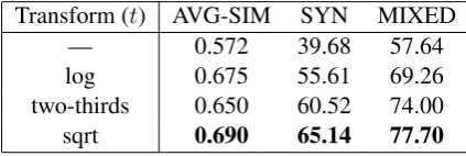
Table 1: Performance of CCA (1000 dimensions) on the development portion of data with different data transformation methods (α= 0.75,β = 0).

as a held-out portion for development and use the other half for final evaluation.

7.1.1 Effect of data transformation for CCA We first look at the effect of different data trans-formations on the performance of CCA. Table 1 shows the result on the development portion with 1000-dimensional embeddings. We see that with-out any transformation, the performance can be quite bad—especially in word analogy. But there is a marked improvement upon transforming the data. Moreover, the square-root transformation gives the best result, improving the accuracy on the two analogy datasets by 25.46% and 20.06% in absolute magnitude. This aligns with the dis-cussion in Section 4.3.

7.1.2 Comparison among different spectral embeddings

Next, we look at the performance of various com-binations in the template in Figure 2. We smooth the context distribution withα = 0.75 for PPMI and CCA. We useβ = 0.5for PPMI (which has a minor improvement overβ = 0) andβ = 0for all other methods. We generally find that using

β = 0is critical to obtaining good performance fors∈ {—,reg}.

Table 2 shows the result on the development portion for both 500 and 1000 dimensions. Even

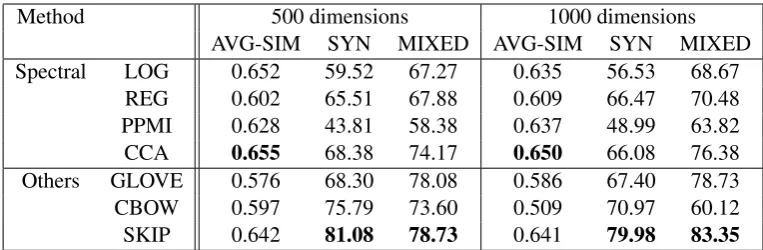
without any scaling, SVD performs reasonably well with the square-root and log transformations. The regression scaling performs very poorly with-out data transformation, but once the square-root transformation is applied it performs quite well (especially in analogy questions). The PPMI scal-ing achieves good performance in word similarity but not in word analogy. The CCA scaling, com-bined with the square-root transformation, gives the best overall performance. In particular, it per-forms better than all other methods in mixed anal-ogy questions by a significant margin.

7.1.3 Comparison with other embedding methods

We compare spectral embedding methods against WORD2VEC and GLOVE on the test portion. We use the following combinations based on their per-formance on the development portion:

• LOG: log transform, — scaling

• REG: sqrt transform, reg scaling

• PPMI: — transform, ppmi scaling

• CCA: sqrt transform, cca scaling

For WORD2VEC, there are two model options: continuous bag-of-words (CBOW) and skip-gram (SKIP). Table 3 shows the result for both 500 and 1000 dimensions.

Method 500 dimensions 1000 dimensions AVG-SIM SYN MIXED AVG-SIM SYN MIXED Spectral LOG 0.652 59.52 67.27 0.635 56.53 68.67

REG 0.602 65.51 67.88 0.609 66.47 70.48 PPMI 0.628 43.81 58.38 0.637 48.99 63.82

CCA 0.655 68.38 74.17 0.650 66.08 76.38

Others GLOVE 0.576 68.30 78.08 0.586 67.40 78.73 CBOW 0.597 75.79 73.60 0.509 70.97 60.12 SKIP 0.642 81.08 78.73 0.641 79.98 83.35

Table 3: Performance of different word embedding methods on the test portion of data. See the main text for the configuration details of spectral methods.

7.2 As features in a supervised task

Finally, we use word embeddings as features in NER and compare the subsequent improvements between various embedding methods. The ex-perimental setting is identical to that of Stratos et al. (2014). We use the Reuters RCV1 cor-pus which contains 205 million words. With fre-quency thresholding, we end up with a vocabu-lary of size around 301k. We derive LOG, REG, PPMI, and CCA embeddings as described in Sec-tion 7.1.3, and GLOVE, CBOW, and SKIP em-beddings again with the recommended default set-tings. The number of left/right contexts is 2 for all methods. For comparison, we also derived 1000 Brown clusters (BROWN) on the same vocabu-lary and used the resulting bit strings as features (Brown et al., 1992).

Table 4 shows the result for both 30 and 50 di-mensions. In general, using any of these lexical features provides substantial improvements over the baseline.6 _{In particular, the 30-dimensional}

CCA embeddings improve the F1 score by 2.84 on the development portion and by 4.88 on the test portion. All spectral methods perform com-petitively with external packages, with CCA and SKIP consistently delivering the biggest improve-ments on the development portion.

8 Conclusion

In this work, we revisited SVD-based methods for inducing word embeddings. We examined a framework provided by CCA and showed that the resulting word embeddings can be viewed as cluster-revealing parameters of a certain model and that this result is robust to data transformation. 6_{We mention that the well-known dev/test discrepancy in} the CoNLL 2003 dataset makes the results on the test portion less reliable.

Features 30 dimensions 50 dimensions Dev Test Dev Test — 90.04 84.40 90.04 84.40 BROWN 92.49 88.75 92.49 88.75 LOG 92.27 88.87 92.91 89.67 REG 92.51 88.08 92.73 88.88 PPMI 92.25 89.27 92.53 89.37 CCA 92.88 89.28 92.94 89.01 GLOVE 91.49 87.16 91.58 86.80 CBOW 92.44 88.34 92.83 89.21 SKIP 92.63 88.78 93.11 89.32 Table 4: NER F1 scores when word embeddings are added as features to the baseline (—).

Our proposed method gives the best result among spectral methods and is competitive to other pop-ular word embedding techniques.

This work suggests many directions for fu-ture work. Past spectral methods that involved CCA without data transformation (e.g., Cohen et al. (2013)) may be revisited with the square-root transformation. Using CCA to induce representa-tions other than word embeddings is another im-portant future work. It would also be interesting to formally investigate the theoretical merits and algorithmic possibility of solving the variance-weighted objective in Eq. (6). Even though the objective is hard to optimize in the worst case, it may be tractable under natural conditions.

Acknowledgments

A Proof of Theorem 4.1

We first define some random variables. Letρ be the number of left/right context words to consider in CCA. Let(W1, . . . , WN) ∈ [n]N be a random sequence of words drawn from the Brown model where N ≥ 2ρ+ 1, along with the correspond-ing sequence of hidden states (H1, . . . , HN) ∈ [m]N_{. Independently, pick a position I ∈ [ρ +} 1, N −ρ] uniformly at random; pick an integer

J ∈ [−ρ, ρ]\{0} uniformly at random. Define

B ∈Rn×n_{,u, v ∈R}n_{,π˜ ∈R}m_{, andT˜ ∈R}m×m as follows:

Bw,c :=P(WI =w, WI+J =c) ∀w, c∈[n]

uw :=P(WI =w) ∀w∈[n]

vc:=P(WI+J =c) ∀c∈[n] ˜

πh :=P(HI=h) ∀h∈[m] ˜

Th0_,h:=P(H_I+J =h0|H_I =h) ∀h, h0 ∈[m]

First, we show thatΩhai_{has a particular structure}

under the Brown assumption. For the choice of positive vectors∈ Rm_{in the theorem, we define}

sh:= (Pwo(w|h)a)−1/2for allh∈[m].

Lemma A.1. Ωhai _=AΘ>_whereΘ∈Rn×m_has rankmandA∈Rn×m_{is defined as:}

A:=diag(Oπ˜)−a/2Ohaidiag(˜π)a/2diag(s)

Proof. Let O˜ := OT˜. It can be algebraically verified that B = Odiag(˜π) ˜O>_{, u = Oπ˜, and}

v = ˜Oπ˜. By Assumption 4.1, each entry ofBhai

has the form

Bhai w,c =

  X

h∈[m]

Ow,h×π˜h×O˜c,h

 

a

=Ow,H(w)טπH(w)×O˜c,H(w)

_a

=Oa

w,H(w)×π˜Ha(w)×O˜c,aH(w)

= X

h∈[m]

Oa

w,h×π˜ha×O˜ac,h

ThusBhai_=Ohai_diag(˜π)a_{( ˜O}hai₎>_{. Therefore,}

Ωhai_=diag(u)−1/2_Bdiag(v)−1/2hai =diag(u)−a/2_Bhai_diag(v)−a/2

=diag(Oπ˜)−a/2_Ohai_diag(˜π)a/2_diag(s) diag(s)−1diag(˜π)a/2( ˜Ohai)>diag( ˜Oπ˜)−a/2

This gives the desired result.

Next, we show that the left component ofΩhai

is in fact the emission matrix O up to (nonzero) scaling and is furthermore orthonormal.

Lemma A.2. The matrixAin Lemma A.1 has the expressionA =Oha/2i_{diag(s)and has} orthonor-mal columns.

Proof. By Assumption 4.1, each entry ofAis sim-plified as follows:

Aw,h = o(w|h)

a_×π˜a/2 h ×sh

o(w|H(w))a/2_×π˜a/2

H(w) =o(w|h)a/2×sh

This proves the first part of the lemma. Note that:

[A>A]h,h0 =

s2 h×

P

wo(w|h)a ifh=h0 0 otherwise Thus our choice ofsgivesA>_A=Im×m. Proof of Theorem 4.1. With Lemma A.1 and A.2, the proof is similar to the proof of Theorem 5.1 in Stratos et al. (2014).

References

Alexander C Aitken. 1936. On least squares and lin-ear combination of observations.Proceedings of the Royal Society of Edinburgh, 55:42–48.

Rie Kubota Ando and Tong Zhang. 2005. A frame-work for learning predictive structures from multiple tasks and unlabeled data. The Journal of Machine Learning Research, 6:1817–1853.

Francis J Anscombe. 1948. The transformation of poisson, binomial and negative-binomial data.

Biometrika, pages 246–254.

MSo Bartlett. 1936. The square root transformation in analysis of variance. Supplement to the Journal of the Royal Statistical Society, pages 68–78.

Peter F Brown, Peter V Desouza, Robert L Mercer, Vincent J Della Pietra, and Jenifer C Lai. 1992. Class-based n-gram models of natural language.

Computational Linguistics, 18(4):467–479.

Danqi Chen and Christopher D Manning. 2014. A fast and accurate dependency parser using neural net-works. InProceedings of the Empirical Methods in Natural Language Processing, pages 740–750. Shay B Cohen, Karl Stratos, Michael Collins, Dean P

Ronan Collobert, Jason Weston, L´eon Bottou, Michael Karlen, Koray Kavukcuoglu, and Pavel Kuksa. 2011. Natural language processing (almost) from scratch. The Journal of Machine Learning Re-search, 12:2493–2537.

Scott C. Deerwester, Susan T Dumais, Thomas K. Lan-dauer, George W. Furnas, and Richard A. Harshman. 1990. Indexing by latent semantic analysis. Jour-nal of the American Society for Information Science, 41(6):391–407.

Paramveer Dhillon, Dean P Foster, and Lyle H Ungar. 2011. Multi-view learning of word embeddings via cca. InProceedings of the Advances in Neural In-formation Processing Systems, pages 199–207. Paramveer S. Dhillon, Jordan Rodu, Dean P. Foster,

and Lyle H. Ungar. 2012. Two step cca: A new spectral method for estimating vector models of words. InProceedings of the International Con-ference on Machine learning.

David Hardoon, Sandor Szedmak, and John Shawe-Taylor. 2004. Canonical correlation analysis: An overview with application to learning methods.

Neural Computation, 16(12):2639–2664.

Harold Hotelling. 1936. Relations between two sets of variates. Biometrika, 28(3/4):321–377.

Erich Leo Lehmann and George Casella. 1998.Theory of point estimation, volume 31. Springer Science & Business Media.

Tao Lei, Yu Xin, Yuan Zhang, Regina Barzilay, and Tommi Jaakkola. 2014. Low-rank tensors for scor-ing dependency structures. InProceedings of the As-sociation for Computational Linguistics, volume 1, pages 1381–1391.

Omer Levy and Yoav Goldberg. 2014a. Linguistic reg-ularities in sparse and explicit word representations. In Proceedings of the Computational Natural Lan-guage Learning, page 171.

Omer Levy and Yoav Goldberg. 2014b. Neural word embedding as implicit matrix factorization. In ceedings of the Advances in Neural Information Pro-cessing Systems, pages 2177–2185.

Omer Levy, Yoav Goldberg, Ido Dagan, and Israel Ramat-Gan. 2015. Improving distributional simi-larity with lessons learned from word embeddings.

Transactions of the Association for Computational Linguistics, 3.

Tomas Mikolov, Kai Chen, Greg Corrado, and Jef-frey Dean. 2013a. Efficient estimation of word representations in vector space. arXiv preprint arXiv:1301.3781.

Tomas Mikolov, Ilya Sutskever, Kai Chen, Greg S Cor-rado, and Jeff Dean. 2013b. Distributed representa-tions of words and phrases and their compositional-ity. InProceedings of the Advances in Neural Infor-mation Processing Systems, pages 3111–3119.

Patrick Pantel and Dekang Lin. 2002. Discover-ing word senses from text. In Proceedings of the ACM SIGKDD international conference on Knowl-edge discovery and data mining, pages 613–619. ACM.

Jeffrey Pennington, Richard Socher, and Christopher D Manning. 2014. Glove: Global vectors for word representation. InProceedings of the Empiri-cial Methods in Natural Language Processing, vol-ume 12.

Nathan Srebro, Tommi Jaakkola, et al. 2003. Weighted low-rank approximations. InProceedings of the In-ternational Conference on Machine learning, vol-ume 3, pages 720–727.

Robert G. D. Steel. 1953. Relation between pois-son and multinomial distributions. Technical Report BU-39-M, Cornell University.