Prototype Driven Learning for Sequence Models

Prototype-Driven Learning for Sequence Models

Aria Haghighi

Computer Science Division

University of California Berkeley

[email protected]

Dan Klein

Computer Science Division

University of California Berkeley

[email protected]

Abstract

We investigate prototype-driven learning for pri-marily unsupervised sequence modeling. Prior knowledge is specified declaratively, by provid-ing a few canonical examples of each target an-notation label. This sparse prototype information is then propagated across a corpus using distri-butional similarity features in a log-linear gener-ative model. On part-of-speech induction in En-glish and Chinese, as well as an information extrac-tion task, prototype features provide substantial er-ror rate reductions over competitive baselines and outperform previous work. For example, we can achieve an English part-of-speech tagging accuracy of 80.5% using only three examples of each tag and no dictionary constraints. We also compare to semi-supervised learning and discuss the system’s error trends.

1

Introduction

Learning, broadly taken, involves choosing a good model from a large space of possible models. In su-pervised learning, model behavior is primarily de-termined by labeled examples, whose production requires a certain kind of expertise and, typically, a substantial commitment of resources. In unsu-pervised learning, model behavior is largely deter-mined by the structure of the model. Designing models to exhibit a certain target behavior requires another, rare kind of expertise and effort. Unsuper-vised learning, while minimizing the usage of la-beled data, does not necessarily minimize total ef-fort. We therefore consider here how to learn mod-els with the least effort. In particular, we argue for a certain kind of semi-supervised learning, which we callprototype-drivenlearning.

In prototype-driven learning, we specify prototyp-ical examples for each target label or label configu-ration, but do not necessarily label any documents or sentences. For example, when learning a model for

Penn treebank-style part-of-speech tagging in En-glish, we may list the 45 target tags and a few exam-ples of each tag (see figure 4 for a concrete prototype list for this task). This manner of specifying prior knowledge about the task has several advantages. First, is it certainly compact (though it remains to be proven that it is effective). Second, it is more or less the minimum one would have to provide to a human annotator in order to specify a new annota-tion task and policy (compare, for example, with the list in figure 2, which suggests an entirely different task). Indeed, prototype lists have been used ped-agogically to summarize tagsets to students (Man-ning and Sch¨utze, 1999). Finally, natural language does exhibit proform and prototype effects (Radford, 1988), which suggests that learning by analogy to prototypes may be effective for language tasks.

In this paper, we consider three sequence mod-eling tasks: part-of-speech tagging in English and Chinese and a classified ads information extraction task. Our general approach is to use distributional similarity to link any given word to similar pro-totypes. For example, the word reported may be linked to said, which is in turn a prototype for the part-of-speech VBD. We then encode these pro-totype links as features in a log-linear generative model, which is trained to fit unlabeled data (see section 4.1). Distributional prototype features pro-vide substantial error rate reductions on all three tasks. For example, on English part-of-speech tag-ging with three prototypes per tag, adding prototype features to the baseline raises per-position accuracy from 41.3% to 80.5%.

2

Tasks and Related Work: Tagging

For our part-of-speech tagging experiments, we used data from the English and Chinese Penn treebanks (Marcus et al., 1994; Ircs, 2002). Example sentences

(a) DT VBN NNS RB MD VB NNS TO VB NNS IN NNS RBR CC RBR RB .

The proposed changes also would allow executives to report exercises of options later and less often .

(b) NR AD VV AS PU NN VV DER VV PU PN AD VV DER VV PU DEC NN VV PU ! " # $ % & ’ ( ) * + , - . / 0 * + , 1 2 3 4 5 6 7

(c) FEAT FEAT FEAT FEAT NBRHD NBRHD NBRHD NBRHD NBRHD SIZE SIZE SIZE SIZE

Vine covered cottage , near Contra Costa Hills . 2 bedroom house ,

FEAT FEAT FEAT FEAT FEAT RESTR RESTR RESTR RESTR RENT RENT RENT RENT

modern kitchen and dishwasher . No pets allowed . $ 1050 / month

Figure 1: Sequence tasks: (a) English POS, (b) Chinese POS, and (c) Classified ad segmentation

are shown in figure 1(a) and (b). A great deal of re-search has investigated the unsupervised and semi-supervised induction of part-of-speech models, es-pecially in English, and there is unfortunately only space to mention some highly related work here.

One approach to unsupervised learning of part-of-speech models is to induce HMMs from un-labeled data in a maximum-likelihood framework. For example, Merialdo (1991) presents experiments learning HMMs using EM. Merialdo’s results most famously show that re-estimation degrades accu-racy unless almost no examples are labeled. Less famously, his results also demonstrate that re-estimation can improve tagging accuracies to some degree in the fully unsupervised case.

One recent and much more successful approach to part-of-speech learning iscontrastive estimation, presented in Smith and Eisner (2005). They utilize task-specific comparison neighborhoods for part-of-speech tagging to alter their objective function.

Both of these works require specification of the legal tags for each word. Such dictionaries are large and embody a great deal of lexical knowledge. A prototype list, in contrast, is extremely compact.

3

Tasks and Related Work: Extraction

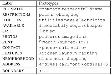
Grenager et al. (2005) presents an unsupervised approach to an information extraction task, called CLASSIFIEDShere, which involves segmenting clas-sified advertisements into topical sections (see fig-ure 1(c)). Labels in this domain tend to be “sticky” in that the correct annotation tends to consist of multi-element fields of the same label. The over-all approach of Grenager et al. (2005) typifies the process involved in fully unsupervised learning on new domain: they first alter the structure of their HMM so that diagonal transitions are preferred, then modify the transition structure to explicitly model boundary tokens, and so on. Given enough

refine-Label Prototypes

ROOMATES roommate respectful drama

RESTRICTIONS pets smoking dog

UTILITIES utilities pays electricity

AVAILABLE immediately begin cheaper

SIZE 2 br sq

PHOTOS pictures image link

RENT $month *number*15*1

CONTACT *phone* call *time*

FEATURES kitchen laundry parking

NEIGHBORHOOD close near shopping

ADDRESS _{address carlmont *ordinal*5}

BOUNDARY ; . !

Figure 2: Prototype list derived from the develop-ment set of the CLASSIFIEDS data. The BOUND-ARY field is not present in the original annotation, but added to model boundaries (see Section 5.3). The starred tokens are the results of collapsing of basic entities during pre-processing as is done in (Grenager et al., 2005)

ments the model learns to segment with a reasonable match to the target structure.

In section 5.3, we discuss an approach to this task which does not require customization of model structure, but rather centers on feature engineering.

4

Approach

In the present work, we consider the problem of learning sequence models over text. For each doc-umentx= [xi], we would like to predict a sequence

of labelsy = [yi], wherexi ∈ X andyi ∈ Y. We

construct a generative model,p(x, y|θ), whereθare the model’s parameters, and choose parameters to maximize the log-likelihood of our observed dataD:

L(θ;D) = X

x∈D

logp(x|θ)

= X

x∈D

logX

y

yi

−1

!DT,NN"

yi

!NN,VBD"

xi

reported

xi−1 witness

f(xi, yi) =

    

   

word=reported

suffix-2=ed

proto=said

proto=had

    

   

∧VBD

f(yi₋₁, yi) =DT∧NN∧VBD

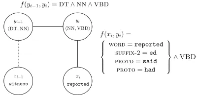
Figure 3: Graphical model representation of trigram tagger for English POS domain.

4.1 Markov Random Fields

We take our model family to be chain-structured Markov random fields (MRFs), the undirected equivalent of HMMs. Our joint probability model over(x, y)is given by

p(x, y|θ) = 1

Z(θ)

n Y

i=1

φ(xi, yi)φ(yi−1, yi)

whereφ(c)is a potential over a cliquec, taking the formexp

θT_{f(c) , andf(c) is the vector of}

fea-tures active over c. In our sequence models, the cliques are over the edges/transitions(yi−1, yi)and

nodes/emissions(xi, yi). See figure 3 for an

exam-ple from the English POS tagging domain.

Note that the only way an MRF differs from a conditional random field (CRF) (Lafferty et al., 2001) is that the partition function is no longer ob-servation dependent; we are modeling the joint prob-ability ofxandyinstead ofygivenx. As a result, learning an MRF is slightly harder than learning a CRF; we discuss this issue in section 4.4.

4.2 Prototype-Driven Learning

We assume prior knowledge about the target struc-ture via aprototype list, which specifies the set of target labelsY and, for each labely ∈ Y, a set of prototypes words,py ∈ Py. See figures 2 and 4 for

examples of prototype lists.1

1_{Note that this setting differs from the standard}

semi-supervised learning setup, where a small number of fully la-beled examples are given and used in conjunction with a larger amount of unlabeled data. In our prototype-driven approach, we never provide a singlefullylabeled example sequence. See sec-tion 5.3 for further comparison of this setting to semi-supervised learning.

Broadly, we would like to learn sequence models which both explain the observed data and meet our prior expectations about target structure. A straight-forward way to implement this is to constrain each prototype word to take only its given label(s) at training time. As we show in section 5, this does not work well in practice because this constraint on the model is very sparse.

In providing a prototype, however, we generally mean something stronger than a constraint on that word. In particular, we may intend that words which are in some sense similar to a prototype generally be given the same label(s) as that prototype.

4.3 Distributional Similarity

In syntactic distributional clustering, words are grouped on the basis of the vectors of their pre-ceeding and following words (Sch¨utze, 1995; Clark, 2001). The underlying linguistic idea is that replac-ing a word with another word of the same syntactic category should preserve syntactic well-formedness (Radford, 1988). We present more details in sec-tion 5, but for now assume that a similarity funcsec-tion over word types is given.

Suppose further that for each non-prototype word type w, we have a subset of prototypes,Sw, which

are known to be distributionally similar tow(above some threshold). We would like our model to relate the tags ofwto those ofSw.

One approach to enforcing the distributional as-sumption in a sequence model is by supplementing the training objective (here, data likelihood) with a penalty term that encourages parameters for which eachw’s posterior distribution over tags is compati-ble with it’s prototypesSw. For example, we might

maximize,

X

x∈D

logp(x|θ)−X w

X

z∈Sw

KL(t|z||t|w)

where t|w is the model’s distribution of tags for word w. The disadvantage of a penalty-based ap-proach is that it is difficult to construct the penalty term in a way which produces exactly the desired behavior.

at eachwfor whichz ∈Sw(see figure 3). One

ad-vantage of this approach is that it allows the strength of the distributional constraint to be calibrated along with any other features; it was also more successful in our experiments.

4.4 Parameter Estimation

So far we have ignored the issue of how we learn model parametersθwhich maximizeL(θ;D). If our model family were HMMs, we could use the EM al-gorithm to perform a local search. Since we have a log-linear formulation, we instead use a gradient-based search. In particular, we use L-BFGS (Liu and Nocedal, 1989), a standard numerical optimiza-tion technique, which requires the ability to evaluate

L(θ;D)and its gradient at a givenθ.

The density p(x|θ) is easily calculated up to the global constant Z(θ) using the forward-backward algorithm (Rabiner, 1989). The partition function is given by

Z(θ) = X

x

X

y n

Y

i=1

φ(xi, yi)φ(yi−1, yi)

= X

x

X

y

score(x, y)

Z(θ) can be computed exactly under certain as-sumptions about the clique potentials, but can in all cases be bounded by

ˆ

Z(θ) =

K

X

`=1

ˆ

Z`(θ) =

K

X

`=1

X

x:|x|=`

score(x, y)

WhereKis a suitably chosen large constant. We can efficiently computeZˆ`(θ)for fixed`using a

gener-alization of the forward-backward algorithm to the lattice of all observations xof length `(see Smith and Eisner (2005) for an exposition).

Similar to supervised maximum entropy prob-lems, the partial derivative ofL(θ;D)with respect to each parameterθj (associated with feature fj) is

given by a difference in feature expectations:

∂L(θ;D)

∂θj

= X

x∈D

Ey|x,θfj−Ex,y|θfj

The first expectation is the expected count of the fea-ture under the model’s p(y|x, θ) and is again eas-ily computed with the forward-backward algorithm,

Num Tokens

Setting

48K

193K

BASE

42.2

41.3

PROTO

61.9

68.8

PROTO+SIM

79.1

80.5

Table 1: English POS results measured by per-position accuracy

just as for CRFs or HMMs. The second expectation is the expectation of the feature under the model’s joint distribution over allx, ypairs, and is harder to calculate. Again assuming that sentences beyond a certain length have negligible mass, we calculate the expectation of the feature for each fixed length`and take a (truncated) weighted sum:

Ex,y|θfj=

K

X

`=1

p(|x|=`)Ex,y|`,θfj

For fixed`, we can calculateEx,y|`,θfjusing the

lat-tice of all inputs of length`. The quantityp(|x|=`) is simplyZˆ`(θ)/Zˆ(θ).

As regularization, we use a diagonal Gaussian prior with varianceσ2

= 0.5, which gave relatively good performance on all tasks.

5

Experiments

We experimented with prototype-driven learning in three domains: English and Chinese part-of-speech tagging and classified advertisement field segmenta-tion. At inference time, we used maximum poste-rior decoding,2which we found to be uniformly but slightly superior to Viterbi decoding.

5.1 English POS Tagging

For our English part-of-speech tagging experiments, we used the WSJ portion of the English Penn tree-bank (Marcus et al., 1994). We took our data to be either the first 48K tokens (2000 sentences) or 193K tokens (8000 sentences) starting from section 2. We used a trigram tagger of the model form outlined in section 4.1 with the same set of spelling features re-ported in Smith and Eisner (2005): exact word type,

2_{At each position choosing the label which has the highest}

Label Prototype Label Prototype

NN % company year NNS years shares companies JJ new other last VBG including being according MD will would could -LRB- -LRB-

-LCB-VBP are ’re ’ve DT the a The RB n’t also not WP$ whose

-RRB- -RRB- -RCB- FW bono del kanji

WRB when how where RP Up ON IN of in for VBD said was had

SYM c b f $ $US$C$

CD million billion two # #

TO to To na : – : ;

VBN been based compared NNPS Philippines Angels Rights RBR Earlier duller “ “ ‘ non-“

VBZ is has says VB be take provide JJS least largest biggest RBS Worst NNP Mr. U.S. Corp. , ,

POS ’S CC and or But

PRP$ its their his JJR smaller greater larger

PDT Quite WP who what What

WDT which Whatever whatever . . ? !

EX There PRP it he they

” ” UH Oh Well Yeah

Figure 4: English POS prototype list

Correct Tag Predicted Tag % of Errors

CD DT 6.2

NN JJ 5.3

JJ NN 5.2

VBD VBN 3.3

NNS NN 3.2

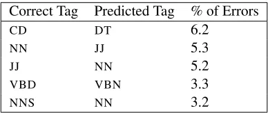
Figure 5: Most common English POS confusions for

PROTO+SIMon 193K tokens

character suffixes of length up to 3,initial-capital, contains-hyphen, andcontains-digit. Our only edge features were tag trigrams.

With just these features (our baseline BASE) the problem is symmetric in the 45 model labels. In order to break initial symmetry we initialized our potentials to be near one, with some random noise. To evaluate in this setting, model labels must be mapped to target labels. We followed the common approach in the literature, greedily mapping each model label to a target label in order to maximize per-position accuracy on the dataset. The results of

BASE, reported in table 1, depend upon random ini-tialization; averaging over 10 runs gave an average per-position accuracy of 41.3% on the larger training set.

We automatically extracted the prototype list by taking our data and selecting for each annotated la-bel the top three occurring word types which were not given another label more often. This resulted

in 116 prototypes for the 193K token setting.3 For comparison, there are 18,423 word types occurring in this data.

Incorporating the prototype list in the simplest possible way, we fixed prototype occurrences in the data to their respective annotation labels. In this case, the model is no longer symmetric, and we no longer require random initialization or post-hoc mapping of labels. Adding prototypes in this way gave an accuracy of 68.8% on all tokens, but only 47.7% on non-prototype occurrences, which is only a marginal improvement over BASE. It appears as

though the prototype information is not spreading to non-prototype words.

In order to remedy this, we incorporated distri-butional similarity features. Similar to (Sch¨utze, 1995), we collect for each word type a context vector of the counts of the most frequent 500 words, con-joined with a direction and distance (e.g +1,-2). We then performed an SVD on the matrix to obtain a re-duced rank approximation. We used the dot product between left singular vectors as a measure of distri-butional similarity. For each wordw, we find the set of prototype words with similarity exceeding a fixed threshold of 0.35. For each of these prototypes z, we add a predicatePROTO=zto each occurrence of w. For example, we might addPROTO=saidto each

token ofreported(as in figure 3).4

Each prototype word is also its own prototype (since a word has maximum similarity to itself), so when we lock the prototype to a label, we are also pushing all the words distributionally similar to that prototype towards that label.5

3_{To be clear: this method of constructing a prototype list}

required statistics from the labeled data. However, we believe it to be a fair and necessary approach for several reasons. First, we wanted our results to be repeatable. Second, we did not want to overly tune this list, though experiments below suggest that tuning could greatly reduce the error rate. Finally, it allowed us to run on Chinese, where the authors have no expertise.

4_{Details of distributional similarity features: To extract}

con-text vectors, we used a window of size 2 in either direction and use the first 250 singular vectors. We collected counts from all the WSJ portion of the Penn Treebank as well as the entire BLIPP corpus. We limited each word to have similarity features for its top 5 most similar prototypes.

5_{Note that the presence of a prototype feature does not}

This setting, PROTO+SIM, brings the all-tokens accuracy up to 80.5%, which is a 37.5% error re-duction overPROTO. For non-prototypes, the accu-racy increases to 67.8%, an error reduction of 38.4% overPROTO. The overall error reduction fromBASE

toPROTO+SIMon all-token accuracy is 66.7%. Table 5 lists the most common confusions for

PROTO+SIM. The second, third, and fourth most common confusions are characteristic of fully super-vised taggers (though greater in number here) and are difficult. For instance, bothJJs andNNs tend to occur after determiners and before nouns. TheCD

andDTconfusion is a result of our prototype list not containing acontains-digitprototype forCD, so the predicate fails to be linked toCDs. Of course in a realistic, iterative design setting, we could have al-tered the prototype list to include a contains-digit prototype forCDand corrected this confusion.

Figure 6 shows the marginal posterior distribu-tion over label pairs (roughly, the bigram transi-tion matrix) according to the treebank labels and the

PROTO+SIM model run over the training set (using a collapsed tag set for space). Note that the broad structure is recovered to a reasonable degree.

It is difficult to compare our results to other sys-tems which utilize a full or partial tagging dictio-nary, since the amount of provided knowledge is substantially different. The best comparison is to Smith and Eisner (2005) who use a partial tagging dictionary. In order to compare with their results, we projected the tagset to the coarser set of 17 that they used in their experiments. On 24K tokens, our

PROTO+SIMmodel scored 82.2%. When Smith and Eisner (2005) limit their tagging dictionary to words which occur at least twice, their best performing neighborhood model achieves 79.5%. While these numbers seem close, for comparison, their tagging dictionary contained information about the allow-able tags for 2,125 word types (out of 5,406 types) and the their system must only choose, on average, between 4.4 tags for a word. Our prototype list, however, contains information about only 116 word types and our tagger must on average choose be-tween 16.9 tags, a much harder task. When Smith and Eisner (2005) include tagging dictionary entries for all words in the first half of their 24K tokens, giv-ing tagggiv-ing knowledge for 3,362 word types, they do achieve a higher accuracy of 88.1%.

Setting Accuracy

BASE 46.4

PROTO 53.7

PROTO+SIM 71.5

PROTO+SIM+BOUND 74.1

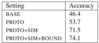
Figure 7: Results on test set for ads data in (Grenager et al., 2005).

5.2 Chinese POS Tagging

We also tested our POS induction system on the Chi-nese POS data in the ChiChi-nese Treebank (Ircs, 2002). The model is wholly unmodified from the English version except that the suffix features are removed since, in Chinese, suffixes are not a reliable indi-cator of part-of-speech as in English (Tseng et al., 2005). Since we did not have access to a large aux-iliary unlabeled corpus that was segmented, our dis-tributional model was built only from the treebank text, and the distributional similarities are presum-ably degraded relative to the English. On 60K word tokens,BASEgave an accuracy of 34.4,PROTOgave 39.0, and PROTO+SIMgave 57.4, similar in order if not magnitude to the English case.

We believe the performance for Chinese POS tag-ging is not as high as English for two reasons: the general difficulty of Chinese POS tagging (Tseng et al., 2005) and the lack of a larger segmented corpus from which to build distributional models. Nonethe-less, the addition of distributional similarity features does reduce the error rate by 35% fromBASE.

5.3 Information Field Segmentation

INPUNC

PRT

TO

VBN

LPUNC

W

DET

ADV

V

POS

ENDPUNC

VBG

PREP

ADJ

RPUNC

N

CONJ INPUNC PR

T

T

O

VBN LPUNC W DET AD

V

V POS ENDPUNC VBG PREP ADJ RPUNC N CONJ

INPUNC

PRT

TO

VBN

LPUNC

W

DET

ADV

V

POS

ENDPUNC

VBG

PREP

ADJ

RPUNC

N

CONJ INPUNC PR

T

T

O

VBN LPUNC W DET AD

V

V POS ENDPUNC VBG PREP ADJ RPUNC N CONJ

(a) (b)

Figure 6: English coarse POS tag structure: a) corresponds to “correct” transition structure from labeled data, b) corresponds toPROTO+SIMon 24K tokens

ROOMATES

UTILITIES

RESTRICTIONS

AVAILABLE

SIZE

PHOTOS

RENT

FEATURES

CONTACT

NEIGHBORHOOD

ADDRESS

ROOMATES

UTILITIES

RESTRICTIONS

AVAILABLE

SIZE

PHOTOS

RENT

FEATURES

CONTACT

NEIGHBORHOOD

ADDRESS

ROOMATES UTILITIES RESTRICTIONS AVAILABLE SIZE PHOTOS RENT FEATURES CONTACT NEIGHBORHOOD ADDRESS

(a) (b) (c)

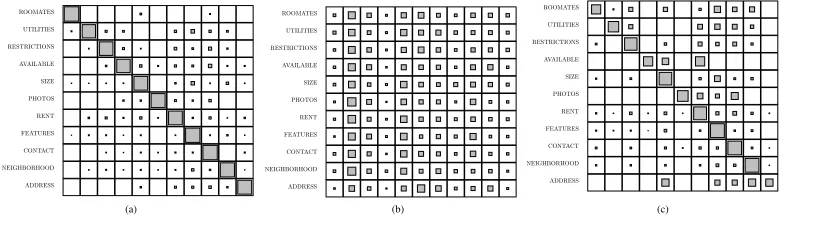
Figure 8: Field segmentation observed transition structure: (a) labeled data, (b) BASE(c)

BASE+PROTO+SIM+BOUND(after post-processing)

figure 8), though we did change the similarity func-tion (see below).

On the test set of (Grenager et al., 2005),

BASEscored an accuracy of 46.4%, comparable to Grenager et al. (2005)’s unsupervised HMM base-line. Adding the prototype list (see figure 2) without distributional features yielded a slightly improved accuracy of 53.7%. For this domain, we utilized a slightly different notion of distributional similar-ity: we are not interested in the syntactic behavior of a word type, but its topical content. Therefore, when we collect context vectors for word types in this domain, we make no distinction by direction or distance and collect counts from a wider win-dow. This notion of distributional similarity is more similar to latent semantic indexing (Deerwester et al., 1990). A natural consequence of this definition of distributional similarity is that many neighboring words will share the same prototypes. Therefore distributional prototype features will encourage la-bels to persist, naturally giving the “sticky” effect of the domain. Adding distributional similarity

fea-tures to our model (PROTO+SIM) improves accuracy substantially, yielding 71.5%, a 38.4% error reduc-tion overBASE.6

Another feature of this domain that Grenager et al. (2005) take advantage of is that end of sen-tence punctuation tends to indicate the end of a field and the beginning of a new one. Grenager et al. (2005) experiment with manually adding bound-ary states and biasing transitions from these states to not self-loop. We capture this “boundary” ef-fect by simply adding a line to our protoype-list, adding a new BOUNDARY state (see figure 2) with a few (hand-chosen) prototypes. Since we uti-lize a trigram tagger, we are able to naturally cap-ture the effect that theBOUNDARYtokens typically indicate transitions between the fields before and after the boundary token. As a post-processing step, when a token is tagged as a BOUNDARY

6_{Distributional similarity details: We collect for each word}

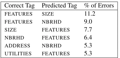
Correct Tag Predicted Tag % of Errors

FEATURES SIZE 11.2

FEATURES NBRHD 9.0

SIZE FEATURES 7.7

NBRHD FEATURES 6.4

ADDRESS NBRHD 5.3

UTILITIES FEATURES 5.3

Figure 9: Most common classified ads confusions

token it is given the same label as the previous non-BOUNDARY token, which reflects the annota-tional convention that boundary tokens are given the same label as the field they terminate. Adding the

BOUNDARY label yields significant improvements, as indicated by the PROTO+SIM+BOUNDsetting in Table 5.3, surpassing the best unsupervised result of Grenager et al. (2005) which is 72.4%. Further-more, ourPROTO+SIM+BOUNDmodel comes close to thesupervisedHMM accuracy of 74.4% reported in Grenager et al. (2005).

We also compared our method to the most ba-sic semi-supervised setting, where fully labeled doc-uments are provided along with unlabeled ones. Roughly 25% of the data had to be labeled in order to achieve an accuracy equal to our

PROTO+SIM+BOUNDmodel, suggesting that the use of prior knowledge in the prototype system is partic-ularly efficient.

In table 5.3, we provide the top confusions made by ourPROTO+SIM+BOUNDmodel. As can be seen, many of our confusions involve theFEATUREfield, which serves as a general purpose background state, which often differs subtly from other fields such as

SIZE. For instance, the parenthical comment:( mas-ter has walk - in closet with vanity )is labeled as a SIZE field in the data, but our model proposed

it as a FEATURE field. NEIGHBORHOOD and AD-DRESS is another natural confusion resulting from the fact that the two fields share much of the same vocabulary (e.g[ADDRESS 2525 Telegraph Ave.]vs.

[NBRHD near Telegraph]).

Acknowledgments We would like to thank the anonymous reviewers for their comments. This work is supported by a Microsoft / CITRIS grant and by an equipment donation from Intel.

6

Conclusions

We have shown that distributional prototype features can allow one to specify a target labeling scheme in a compact and declarative way. These features give substantial error reduction on several induction tasks by allowing one to link words to prototypes ac-cording to distributional similarity. Another positive property of this approach is that it tries to reconcile the success of sequence-free distributional methods in unsupervised word clustering with the success of sequence models in supervised settings: the similar-ity guides the learning of the sequence model.

References

Alexander Clark. 2001. The unsupervised induction of stochas-tic context-free grammars using distributional clustering. In

CoNLL.

Scott C. Deerwester, Susan T. Dumais, Thomas K. Landauer, George W. Furnas, and Richard A. Harshman. 1990. In-dexing by latent semantic analysis.Journal of the American Society of Information Science, 41(6):391–407.

Trond Grenager, Dan Klein, and Christopher Manning. 2005. Unsupervised learning of field segmentation models for in-formation extraction. InProceedings of the 43rd Meeting of the ACL.

Nianwen Xue Ircs. 2002. Building a large-scale annotated chi-nese corpus.

John Lafferty, Andrew McCallum, and Fernando Pereira. 2001. Conditional random fields: Probabilistic models for seg-menting and labeling sequence data. InInternational Con-ference on Machine Learning (ICML).

Dong C. Liu and Jorge Nocedal. 1989. On the limited mem-ory bfgs method for large scale optimization. Mathematical Programming.

Christopher D. Manning and Hinrich Sch¨utze. 1999. Founda-tions of Statistical Natural Language Processing. The MIT Press.

Mitchell P. Marcus, Beatrice Santorini, and Mary Ann Marcinkiewicz. 1994. Building a large annotated corpus of english: The penn treebank. Computational Linguistics, 19(2):313–330.

Bernard Merialdo. 1991. Tagging english text with a proba-bilistic model. InICASSP, pages 809–812.

L.R Rabiner. 1989. A tutorial on hidden markov models and selected applications in speech recognition. InIEEE. Andrew Radford. 1988. Transformational Grammar.

Cam-bridge University Press, CamCam-bridge.

Hinrich Sch¨utze. 1995. Distributional part-of-speech tagging. InEACL.

Noah Smith and Jason Eisner. 2005. Contrastive estimation: Training log-linear models on unlabeled data. In Proceed-ings of the 43rd Meeting of the ACL.