Trinity College Dublin
School of Computer Science and Statistics
M.Sc in Computer Science
Partitioning POMDPs for multiple input types, and
their application to dialogue managers
Author:
Grace
Cowderoy
Supervisors:
Dr. Carl
Vogel
Dr. John
Kelleher
Prof. Nick
Campbell
Partitioning POMDPs for multiple
input types, and their application
to dialogue managers
Approved by Dissertation Committee: Saturnino Luz
Declaration
I declare that this report details entirely my own work. Due acknowledgements and references are given to the work of others where appropriate. I agree to deposit this thesis in the University’s open access institutional repository or allow the Library to do so on my behalf, subject to Irish Copyright Legislation and Trinity College Library conditions of use and acknowledgement.
Grace Cowderoy
Abstract
This research looks at the POMDP models used for dialogue management within Spoken Dialogue Systems (SDS). In particular, it examines the difficulty of handling multimodal inputs. It proposes a generalisation of the POMDP model in order to tackle this.
Contents
1 Introduction 1
1.1 Spoken Dialogue Systems . . . 1
1.2 Aims . . . 2
1.3 Significance of Study . . . 2
1.4 Outline of Thesis . . . 3
2 Current Literature 4 2.1 Human-Computer Interactions . . . 4
2.1.1 Mutual Understanding . . . 6
2.2 Mathematics of POMDPs . . . 8
2.2.1 Policies . . . 10
2.3 Literature Review . . . 12
2.4 Current problems . . . 14
3 Partitioning the POMDP 17 3.1 Learning a POMDP . . . 17
3.2 Motivation for Partitioning . . . 18
3.3 Partitioning the POMDP state space . . . 20
3.3.1 Defining the model . . . 20
3.3.2 Update Function . . . 21
3.3.3 Dependent Partitions . . . 22
3.3.4 Theoretical Results . . . 23
4 Evaluation 25 4.1 Programming the model . . . 26
4.2 Comparison software . . . 26
4.3 Results . . . 27
5 Conclusion 29
5.1 Future Work . . . 30 5.2 Final Remarks . . . 31
List of Figures 32
Bibliography . . . 33
Chapter 1
Introduction
This dissertation looks at the current methods and procedures of spoken dialogue systems such as Siri or Cortana. It discusses how humans and computers interact. In particular, it focuses on the mathematics behind how computers decide how to respond to an input which may or may not be human. The dissertation then proposes a method to improve on the limits of the current mathematical model. This method can be used with multiple input modules, such as microphones, webcams or laser sensors. This method is evaluated with a simulation of three input modules. In the evaluation, the time taken to make the decision via this method is one-third of the time needed via current methods. The following section 1.1 introduces the concept of a dialogue system, and briefly mentions imple-mentations of such systems.
1.1
Spoken Dialogue Systems
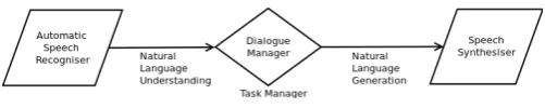
A spoken dialogue system is a program which communicates with a human through speech, and is also known as a Speech Dialogue System (SDS). Spoken dialogue systems are expanding in use, with common deployments including call centres and voice interfaces such as Apple’s Siri. A basic spoken dialogue system is made up of six main components (Jurafsky et al., 2000, p. 857), as seen in Figure 1.1. These are as follows:
• An Automatic Speech Recogniser (ASR), which takes input from the microphone and transcribes
it;
• A Natural Language Understanding component (NLU);
• A Dialogue Manager;
• A Task Manager;
Figure 1.1: Diagram of a SDS
• A Text-to-Speech synthesiser, which realises the text output from the NLG as sound and plays it through the speakers.
A common deployment of a SDS is in a call centre, to handle basic tasks, such as fielding the call to the correct department. This deployment can make use of a task-based approach that is suitable for rule-based or frame-based systems. These are often based on a single sensor: the verbal phone input. A key problem is the noise that the ASR must deal with, and the resulting uncertainty that can cause difficulties for the dialogue manager.
More recently, spoken dialogue systems have provided an interface with mobile devices, with Apple’s Siri being the most recognisable example. Unlike a call centre, a smart device may have multiple types of sensory information available to it, such as a camera; physical orientation; heart rate sensor; etc. Previous multimodal systems, such as the SEMAINE toolkit (Schr¨oder, 2010) force the sensory input to be combined before the information is passed to the dialogue manager. Similarly, dialogue managers to date have required the infomation to be combined. Young (2010) on Cognitive User Interfaces shows that a Partially Observable Markov Decision Process (POMDP) may be applied to sensors other than ASR, but this requires an individual POMDP for each sensor.
1.2
Aims
While spoken dialogue systems are widely implemented, at present they are restricted to a singular input type. Typically, this is automatic speech recognition. The aim of this thesis is to examine how current models may be expanded to handle multiple inputs in modular form. This is done by evaluating a mathematical model called Partially Observable Markov Decision Processes (POMDPs) for tractability, and partitioning it in order to handle modular inputs.
1.3
Significance of Study
such as collision detection which requires three-dimensional motion, being able to handle multiple modular inputs is of significant value, as it allows the system to expand beyond current POMDP solver software.
1.4
Outline of Thesis
Chapter 2
Current Literature
This chapter discusses human-computer interaction, and introduces a mathematical model type called Partially Observable Markov Decision Processes (POMDPs). The chapter starts by discussing human-computer interaction, and the motivations for using a dialogue interface. In subsection 2.1.1, the issues that dialogue managers face are discussed, notably ambiguity. The many sources of ambiguity are considered in relation to dialogue managers, and how they handle and resolve uncertainty. Then, section 2.2 formally defines the POMDP model, and is extended by subsection 2.2.1, which discusses the concept of a policy. A policy is determined for a specific POMDP, and directly affects the outcome of the POMDP.
The chapter then summarises the history and motivation of POMDPs as dialogue managers. It looks at how POMDPs have been trained from data in order to produce a dialogue manager. It then looks at the computational complexity of calculating an optimal policy for a given POMDP, and discusses approximation techniques for calculating an optimal policy. Other examples of the POMDP structure used for dialogue management are examined, particularly variations of the POMDP structure, or where it is combined with other techniques.
The chapter then moves on to consider current problems with the state-of-the-art approach. In particular, it considers the issues of when a system has multiple modules of input. The key problem raised here is that of scaling - that each possible combination of states from each of the inputs must have its own state under the standard POMDP model. This results in an extremely large state-space. The final section introduces concepts needed to understand the model which is proposed in the next chapter, in order to address these problems.
2.1
Human-Computer Interactions
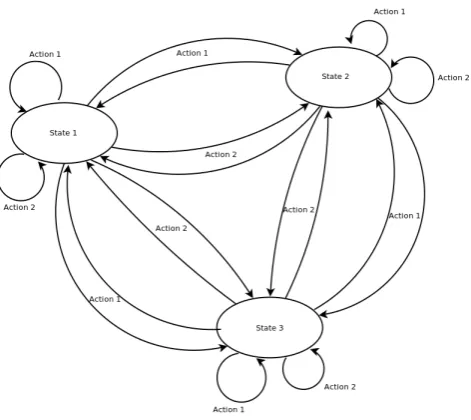
Figure 2.1: Diagram of a Markov Decision Process
been deployed within smart mobile devices, but there is a great deal more to be done within the field of Human-Computer Interaction. While graphical user interfaces (GUIs) have been the base of most human-computer interaction for the past twenty years, they require the visual focus of the user. Moving towards a dialogue interface reduces this dependency on the visual focus, allowing it to be used in more scenarios, such as situations that must be hands-free. The dialogue manager is an important aspect of a SDS. Its role is to decide, given the input from the NLU component, what the output of the NLG should be. Initially, dialogue managers were rule-based systems of if-then statements. Each possible scenario that the system might encounter needed to be coded individually. The simplest type of dialogue manager uses a finite-state machine (sometimes called a finite state automaton, or FSA) as the underlying architecture. In these, there is a flow-chart style diagram which the dialogue runs through, with no variation beyond the paths allowed by the FSA, and no flexibility. In effect, the system controls the conversation. My work makes use of a statistical model, a Partially Observable Markov Decision Process (POMDP), which takes into account input in addition to the ASR. A POMDP is more flexible than a FSA, since it takes into account the possibility that the observed input was flawed. This is a result of the observation function (section 2.2). My model further allows for the input from multiple independent streams, in order to reduce the noise of the observed inputs.
with a set of statesS that the system may be in; a set of actions Athat the system may take; and a reward functionr:A×S→R,denoted asr(a, s), that rewards the system for taking an actionafrom states. A stateiis called an absorbing state if, once the system is in stateiit will remain ini. That is, ifP(Xt+1 =i|Xt=i) = 1, theniis an absorbing state. This means that the system, once in this state, will never leave, asP(Xt+2=i|Xt+1=i) =P(Xt+1=i|Xt=i) = 1, and similarly for all future states. If P(Xt+1 =i|Xt=i)<1, then the state is not an absorbing state, by definition. Typically, one assumes that the system terminates on absorption. Initialising the MDP will designate one of the states as the start state. The reward is accumulated by the system over each time step, and the final cumulated reward may be viewed as how well the system performed. In order to maximise the total reward accumulated, a policy is used (subsection 2.2.1). A decision rule dictates to the system which actiona to take when it is in a given states. A policy is a set of decision rules. Figure 2.1 shows a basic MDP without a reward function, with 3 states and 2 actions available to the system. An example reward functionR :S×A→R might define the following: R(s1, a1) = 10 and R(s1, a2) = 1. This would bias the system towards taking actiona1 from states1 over taking actiona2 if large positive values are preferred. R would be defined for alls∈S anda∈A. However, there is still a possibility that the system will take some other action, (determined by the policy and whether short-term or long-term gains are preferred.) What action the system takes is determined by the policy, which can be adjusted to favour short-term or long-term gains. Note that the reward is dependent on the state that the system is in when it takes the action, but independent of the state that the system moves to.
Like the rule-based systems, MDPs rely on the input being dependable, despite the many potential sources of error. The MDP system believes that at each time point, it is in a single specific state, with no possibility of being in a different one. However, this contradicts a key feature of natural human-human dialogue: dialogue is uncertain.
2.1.1
Mutual Understanding
mind of the user. The intentions and goals of the user, inferred via the realised words, are treated by the dialogue manager as states. In this way, the dialogue manager attempts to model the goals of the user from the observed input received.
However, ambiguity of language is not the only issue that human-human conversation must handle. In human-human dialogue, a technique called common ground, discussed by Clark (1996), can be used to maintain disambiguation of language, but also handle established conventional meanings within communities of practice. Thus, utterances that are particular to a community or dialect are understood by those belonging to that community, but also serve as markers of identity as members of that community. As such, the knowledge of the community may impact the understanding of the utterance. Analogously for the dialogue manager, this means that the user model that provides input into a dialogue system could affect how an utterance is understood. Hence, the inaccuracy of the user model could introduce uncertainty into the system.
Another source of uncertainty within human-human dialogue is that of the utterer’s meaning. Grice (1989) has a theory of utterer’s meaning which distinguishes between what is said; what is implicated conventionally; and what is implicated for conversation. The interaction of these types of meaning can lead to uncertainty as to which meaning is actually intended. For a dialogue system, this means that the output of the Natural Language Understanding component may contain a meaning other than what was intended by the utterer. This in turn compounds the uncertainty that the dialogue manager must deal with.
The uncertainty discussed above is inherent to human-human conversation. When a computer is introduced to play the role of one of the participants, further uncertainty is introduced. As men-tioned, which meaning is inferred by the Natural Language Understanding component can introduce uncertainty. This uncertainty may be greater than when humans converse, since humans are better at identifying which meaning is implied by the utterer. Other technical sources of uncertainty includes how the input speech signal is processed, which can affect the performance of the ASR. This may also be affected by the accent of the utterer and the amount of background noise.
to what is already known by the system. The system makes its decisions dependent on the belief state, which can be considered as the distribution over user possible user intents, with the highest probability corresponding to the most likely user intent. This handles the uncertainty better, since every input is considered relative to what was previously uttered by the user and by the system, so increasing the robustness of the system. The mathematics of POMDPs are further described below in section 2.2.
2.2
Mathematics of POMDPs
A partially observable Markov Decision process (POMDP) is a stochastic process - a mathematical system which varies with respect to timet∈N.
For any set ∆ ⊆R, a collection {Xt: t∈ ∆} of random variables is called a stochastic process. Note that a POMDP works in discrete time units, so here one may consider ∆ =N. A POMDP is a Markov process, which means that the Markov property holds. This property states that, conditional on the present, the future is independent of the past. Denote the probability of eventA occurring as
P(A).
A stochastic process {Xt, t= 0,1,2, ...}is called a Markov process if for non-negative integerss, t and any collection of states (x0, x1, x2, ...) the following probability holds:
P(Xt+s=xt+s|Xt=xt, Xt−1 =xt−1, ..., X0 =x0) =P(Xt+s=xt+s|Xt=xt). This is known as the Markov Property. Note that the Xt−1 =xt−1, ..., X0 =x0 term dependencies on the left-hand side are discarded in the right-hand side. This is equivalent to saying that, conditional on the present, the future is independent of the past. Equivalently, what happens tomorrow depends on what happens today. What happens today depends on what happened yesterday, but what happens tomorrow does not depend on what happened yesterday.
A basic diagram of a POMDP can be seen in Figure 2.2. Here, the POMDP has 3 states and 2 actions like the earlier MDP (Figure 2.1), but is faded out because we do not know exactly which state the system is in. The observations are used to form a statistical distribution, represented in the image by the bar chart, which denotes the belief state. The policy is then consulted, and this determines which action should be taken. The action then feeds back into the POMDP for the next time state.
Formally, a POMDP is a tuple, {S, A, T, R, O, Z, λ, b0}, where:
1. S is a set of states;
2. A is a set of actions;
3. T is a transition function, T :S×A→S;
4. R is a reward function,R:S×A→R;
Figure 2.2: Diagram of a POMDP
6. Z is a observation function;
7. λis a discount factor; and
8. b0is the initial belief state
A POMDP has a set of statesS (item 1) which describe the world in which it operates. However, at any given point in time after initiation of the system (t >0), the state which the system is in may not be known exactly. Instead, the state is inferred from the inputs received about its external world. These inputs are called ‘observations’O (item 5) and the probability of receiving a certain inputois considered with respect to the states, so allowing the system infer from the observation which state the system is most likely to be in.
However, since this is a probability, the system maintains a distribution over the states. This distribution is referred to as the ‘belief state’ for each time unit.
More formally, the belief state at timet,btis a vector ofmdimensions, wheremis the number of states in the system. That is to say,bt= (bt1, bt2, ..., btm). Note that for given timet,∀i∈S,bti ∈[0,1], andbti is the probability of the system being in stateiat time t. Thus,P
ib t
i= 1 at all time unitst. The initial belief state,b0 (item 8) is predetermined and part of the initialisation process. There-after, for time t > 0, the belief state depends on the initial belief state, the actions taken, and the observations received.
The parameters of the distribution can change with time. For example, b0 could be the uniform distribution, but at some later time the distribution bt might morph to show peaks for particular states.
The POMDP accepts inputs from its external world, which are referred to as observations. In the context of a dialogue manager, these observations may come from ASR, facial recognition, or any sensory input where the signal has been processed. The system can perform actions from the set A
(item 2) which may affect its world. These may include applying a parser, waiting a period of time, or outputting a message to a synthesiser.
in a given belief state. A policy is a tree of decision rules, dictating what the system should do for each belief state (subsection 2.2.1). This tree allows for the different possible observations that might be received by the system, but for a realised sequence of belief states and observations, one sequence of the branching process is actually followed. Typically, the policy is calculated offline ahead of implementing the POMDP, and aims to maximise the total expected reward, as dictated by the reward function (item 4).
It is possible to bias a system towards certain actions by specifying the reward functionR(item 4) to do so. This can be considered as giving the system “points” for taking a certain action from a certain belief state.
For each action, from each state, there is a probability to go to each other state. These probabilities are determined by the transition matrixT (item 3). Similarly, for each observation and action-state pair, there is a probability of what the next state is. These probabilities form the observation matrix
Z (item 6). The variableλ(item 7) is the discount factor, which affects the reward function. It helps prevent the system from remaining in one (undesired) state or in a loop, if the states involved are not termination or absorbing states. It works by reducing a proportion of the reward given the system at each time step. This works to balance whether the system will favour immediate rewards or long term rewards.
2.2.1
Policies
White (1993, p. 26) writes that for Markov Decision Processes “a decision rule δt for time unit t determines a probability distribution of actions a ∈ A when the history is known ... a policy is a sequence of decision rules. A policy is denoted by π and takes the form π = (δ1, δ2, ., ., ., ., .δt, ., .)” Note that each policyπmaps from a belief state to the set of actions A, i.e. π:bt→A.
Crucially, a policy informs the system what action to take at any time unit of the decision process. In section 2.2, the reward function, R : S ×A → R was introduced. As stated there, the reward function can be used to bias the system towards certain actions. This is done by calculating an optimal policy, which is one which maximises the expected total reward.
For the firstntime units, let Θ denote the cumulative discounted reward, wherert is the realised reward, Θ =Pn
t=1λ
trt. The expected return,
E(Θ) is dependent on the realised reward,rt, which in turn depends on the belief state and on the policyπwhich dictates which belief states may realistically be achieved. Note that not all belief states may be achieved from the initial belief state, b0. Only those belief states which may, through a finite sequence of actions be realised, are achievable. Further, as some actions and observations are more probable than others, some belief states are significantly unlikely to occur.
Vπ(b) =P∞
t=0λ tr(b
t, at) =P∞t=0
P
si∈Sb t
ir(si, a) =P∞t=0
P
si∈Sb t
ir(si, π(bt)),
wherebtis the distribution over all states at time t, andbti is the probability of the system being in statesi at time t.
The performance of the system is dependent on the policy, as the value function depends on the policy. An optimal policy π∗(b), whereπ∗(b)∈A, is one that maximises the value function. Within a spoken dialogue system, a POMDP dialogue manager will perform best when its policy is optimal. Thus, the computational tractability of calculating the optimal policy is relevant. Papadimitriou & Tsitsiklis (1987) demonstrated that calculating the optimal policy exactly is PSPACE-hard, dependent on the state-space|S|. This places the problem in the same complexity class as several other problems, listed by Garey & Johnson (1979), such as the equivalence problem for non-deterministic finite state automata (determining whether two automata A1, A2 accepting the same input alphabet Σ, where Σ≥2 recognise different languages). More importantly, it is in the NP complexity class. Algorithms exist to calculate the optimal policy exactly, such as Kaelbling et al. (1998), but these swiftly become impractical when|S|+|O| ≥23, which took 2 hours to calculate on machines in the 1990s (Littman et al., 1995). This is because the belief space grows exponentially. However, the lack of tractable exact algorithms does not prevent POMDPs being used as dialogue managers. A number of algorithms exist to calculate an approximation to the optimal policy, beginning with the Point Based Value Iteration algorithm introduced by Pineau et al. (2003), which was applied to a POMDP with 870 states, 5 actions and 30 observations. Approximation algorithms restrict the belief space to reachable belief states – those beliefs that are possible from the current belief state. More recent algorithms include the SARSOP algorithm, introduced by Kurniawati et al. (2008). Work in reinforcement learning has also looked at ways to improve the way the reward function is defined. More details can be found in section 2.3. Whilst the policies learnt from approximation algorithms are not the exact optimal policy, they are usable within dialogue managers. Thomson et al. (2007) adapted a technique for MDPs, Q-learning, to approximate a policy for a tourist information domain dialogue manager. Within this domain, the learnt policy successfully completed 90.6% of the 160 dialogues. The main drawback of the Q-learning technique is the several thousand dialogues needed to train the policy initially. Typically, this learning needs to be done in advance, but may be combined with reinforcement learning for further improvement.
2.3
Literature Review
The history of POMDPs is a long one. They originated out of operations research, in particular the design of control systems (˚Astr¨om, 1965), as an expansion of Markov Decision Processes. The motivation then was to handle situations when the state variables could not be measured, and were not completely observable. This applies to a number of situations, dialogue as one of them. Outside the field of human-computer interaction, POMDPs have been successfully implemented in a variety of fields. These include collision detection in unmanned aerial vehicles, (Temizer et al., 2010); in treatment of heart disease, (Hauskrecht & Fraser, 2000); and conserving endangered species, (Chad`es et al., 2008). Having mentioned these other areas which make use of POMDPs, the rest of this section will focus on the history of POMDPs within dialogue systems.
The use of Partially Observable Markov Decision Processes (POMDPs) as dialogue managers began with the paper by Williams & Young (2007). This paper gave examples of a POMDP being used as a statistical model base for a dialogue manager and marked a shift towards statistical dialogue managers with POMDPs providing the core model. The motivation for this was to handle the input from automatic speech recognisers which were, and remain, unreliable. The main advantage of using a POMDP is that the model takes into account the notion that the observations received may be uncertain, as it considers the probability of receiving that observation. A POMDP gives more flexibility over the more tractable Markov Decision Process (MDP) which assumes that the exact state is known exactly at all times. The motivation was built upon further by Young et al. (2010), which described the mathematics of POMDPs. Like Williams & Young (2007), Young et al. (2010) model the user intent as the states of the POMDP, an approach which was followed by later work, including Chinaei & Chaib-draa (2011) and Yoshino & Kawahara (2014).
The literature that builds on Williams & Young (2007) has been in three broad areas: the training of states, actions, observations and transition function from a corpus; the problem of approximating policies; and implementing POMDP models as dialogue managers.
POMDP.
Papadimitriou & Tsitsiklis (1987) demonstrated that calculating the optimal policy with respect to the reward function is intractable; more specifically, it isP SP ACE-hard. However, the Point-Based Value Iteration (PBVI) algorithm, introduced by Pineau et al. (2003) provided the first algorithm that approximated an optimal policy, allowing it to scale to real-world-sized problems. Point Based Value Iteration (PBVI) selects a number of points in the belief space and calculates the value function of these points. It maintains a backup operator in order to calculate the value function at timet. This backup operator is then modified to retain a singleα-vector for each belief point. Later algorithms include the SARSOP algorithm described by Kurniawati et al. (2008) which adapted PBVI to optimally reachable belief spaces; and adaptions of Q-learning for MDPs Thomson et al. (2007) were evaluated against PBVI. (Kurniawati et al., 2008, p. 2) describe PBVI as “the first point-based algorithm that demonstrated good performance on a large POMDP called Tag, which has 870 states.” This particular POMDP was based in the robotic domain and was inspired by the game of lasertag. Kurniawati et al. (2008) also mention two other point-based algorithms, HSVI2 and FSVI, on which their SARSOP algorithm is based. Thomson et al. (2007, p.11) offer an alternative approach for approximating a policy that differs from the point-based approaches discussed earlier. Instead, the approach is based on Q-learning, which the authors describe as “a technique for online learning traditionally used in an MDP framework” that is in the Monte-Carlo style iterative algorithm.
However, the method of defining the reward function in Williams & Young (2007) was manual. Conservatively, actions that were desired were given a positive reward, and those that were not were discouraged with negative values by the reward function. Frequently, in a real world scenario, the reward function is unknown, but observable (Cao & Guo, 2004). However, whilst reward functions which mimic the observed reward are of interest, since they affect the policy and the behaviour of the POMDP, they are not the focus of discussion here.
One approach to handling the many different concepts that are combined in dialogue managers is in the work of Varges et al. (2011). In this work, a different POMDP was implemented for each task, each with its own policy. A task-structure controller was used to determine which POMDP was active. This controller was a AND-OR graph with a common root node - effectively a strict hierarchy of multiple POMDPs. This hybrid structure, whilst relatively tractable, requires that the controller has understood the ASR correctly in order to pass control to the correct POMDP. This negates the motivation of using a POMDP: that what is understood about the world is known to be a flawed understanding.
Others have looked at partitioning a POMDP, notably Hsiao et al. (2007). However, their work focussed on moving a robot around a two dimensional space, not a speech dialogue system. Also, while they use the term ‘partition’, this is in reference to regions of a single state space where the probability of being in that region is high. This affects the belief state, which may have a high certainty of being in a particular region. However, in this scenario, there is only one input type, which is the contact status of the robot sensor. As such, whilst dividing the belief state into such regions has computational advantages, the concepts in this paper are different to those presented below for maintaing a partition for each feature set.
2.4
Current problems
As section 2.3 explains, whilst POMDPs have been used as dialogue managers since 2007, there remains a problem of tractability when the model is scaled to a large state space. Attempts to handle this have formed hybrid systems, but these fail to take full advantage of the flexibility and uncertainty handling that the POMDP provides. Hybrid systems require that the correct POMDP is chosen by a rule-based controller, which struggle with faulty ASR.
One example of a hybrid system is Wu et al. (2015), which used a POMDP dialogue manager as a means of knowledge acquisition via slot-filling. To better handle the uncertainty introduced by the ASR, they used an N-best list as a distribution of the observations. In their work, they used humans to teach the system properties of various objects. They divided the 128 user goals into four sets, and noted that|Su|is the size of the Cartesian product of the four sets (six sets of two elements each, and a further two sets of one element each.) They consider a total of 3841 states,s= (su, au, sd) plus an absorbing state, wheresd is the dialogue history, andau is the user action. The POMDP agent has 134 actions available to it.
In the research on dialogue managers to date, there have been two main approaches: hand-crafted finite-state automata (FSA), and the statistical approach of MDPs and POMDPs (Williams & Young (2007), Young et al. (2013), Thomson et al. (2007)). It certainly has advantages over previous rule-based models such as FSAs or slot-filling models due to its flexibility, and over the more tractable Markov Decision Process model due to its handling of uncertain input.
against a hand-crafted FSA and against a POMDP trained on a Wizard-of-Oz system. The task was for the human user to instruct a Nao robot to traverse a maze with imaginary rules and to manipulate a graspable object. The dialogues evoked by the three systems were evaluated on 15 metrics, of which 9 were objective and 6 subjective. The objective evaluations included average number of repetitions, average number of turns, and overall dialogue duration. The subjective measures were the multiple answer questions from the user survey.
However, in expanding dialogue managers to handle multiple tasks, the POMDP does not make best use of all the information that is available to it. Currently, dialogue managers have any multi-modal features combined into a vector before the POMDP model receives the state. That is, for each feature f ∈ F and g ∈ G, the multimodal feature is treated as the vector (f, g). This necessitates a large state space, because every possible combination of features requires its own state. In turn, this makes updating the belief function less tractable, since to update the belief function, one must calculate for each state the probability of being in that state. Thus forFi, i∈I whereI is an index set (a set used to label the collection of feature sets) andFiis a set of features, the state space needed by the POMDP isQ
i∈I|Fi|. This means that scaling remains an issue. Due to the large state space required, sensitivity to a given feature within a state is reduced, because it competes with other states which have the same feature in alternative combinations.
In the model I propose below, the state space remains partitioned by the input features. The overall state space can be considered as a function of these partitions. This means that the number of states over which the system must maintain a belief distribution is reduced, since each input feature set is considered with its own distribution. Thus, the uncertainty of each input type is independent from the uncertainty from other input types. Wherever there are actions which do not affect at least one input type, there is a reduction in the number of calculations needed to update the belief state. This increases overall tractability.
By retaining the partitions of the state space, the sensitivity to different features increases, since each distribution is over a smaller number, so any deviation from the expected distribution is more noticeable. Also with these partitions of the state space, the weightings on the feature sets can be dynamic, adjusted depending on what information comes from each input feature. As a result of the increased sensitivity, the actions could be adjusted to target a single feature set, and the POMDP policy can be adjusted to reflect this. This model is a version of a POMDP, which means that unlike the hybrid systems described earlier, it retains the flexibility to move between states in the partition. Also, it handles the uncertainty of the inputs because it does not require a rule-based controller to determine whether a partition should be in focus.
The intuition behind this is that knowing the component pieces gives information about the combi-nation of them. For example, consider a course that is assessed via continuous assessment (component
knowing f(c, e). The reverse may not be. That is to say, knowing f(c, e) does not give information about c or e. Also, if a distribution over C is available, then identifying deviation of c from the distribution is possible. Likewise with E. Further, it is possible to identify deviation between the distributions overC andE.
Chapter 3
Partitioning the POMDP
This chapter briefly looks at how a POMDP model can be trained from data, based on the literature and my own work to apply the method to a different corpus. The motivation for training a POMDP from data is that it makes the states of the POMDP directly correlate to the corpus it is trained on, rather than being formed by handcrafting. The chapter then looks at motivation for partitioning a POMDP for modular input. The main motivation is to reduce computational costs. Partitioning the POMDP allows the total number of states to be reduced. This reduces the costs associated with simulating a POMDP. A secondary motivation is to reduce the noise in the system. Partitioning maintains a separation of the input methods. This means that the system can use each input type independently. The system can also use the alternative input types to resolve uncertainty. For example, the separation allows the system to detect when there are discrepancies between the input types. These discrepancies could hold further information, such as when ASR and prosodic information are in conflict may indicate sarcasm.
3.1
Learning a POMDP
Hidden Topic Markov Models (HTMMs) were introduced by Gruber et al. (2007) for modelling the words in a text corpus as topics, by combining Latent Dirichlet Allocation with Hidden Markov Models. Chinaei et al. (2009) adapted this method to dialogue corpora, with the motivation that the topics which are learnt by the HTMM are correlated to the intention encoded within user utterances. Chinaei & Chaib-draa (2011) apply this method to the SACTI corpus of wizard-user dialogues. Here, learning the topics via an HTMM to represent the user intention, the topics are then used as the states of a POMDP, in accordance with Williams & Young (2007), where the states represent the user ‘goal’ or intent.
successful than with four topics. A naive Bayes classifier was used to assign topics to utterances. The dialogue moves that were included in the annotated maptask were treated as the actions and the observations when performed by the follower and the guide respectively. These were aligned with the utterances in order to calculate the transition matrix and the observation matrix. The entries in the matrix was calculated as follows: T(s1, a1, s2) =
count(s1,a1,s2)+1
count(s1,a1)+K where K =|S|. This is adjusted from Chinaei et al. (2009) in order to ensure that each row of the transition matrix sums to 1, which the APPL software by Kurniawati et al. (2008) checks prior to approximating a policy.
3.2
Motivation for Partitioning
Having trained a POMDP on dialogue data, one questions whether it is possible to expand this model and training to multiple modular inputs. When humans interact, there is more than what words are said; there is information in how they are said. An effective dialogue system should be able to handle this extra information. Recall that Figure 1.1 represents a SDS, and note that a POMDP dialogue manager is designed to only handle a single input type: from the ASR. As areas such as gesture recognition and facial recognition improve, these provide other input streams which might be used to reduce the noise from the ASR input. These streams will also have inherent uncertainties, but these uncertainties may be different from those of the ASR. The model I propose handles these multiple input streams within the dialogue manager itself, and is designed to accept any number of input types, not just the single ASR input currently accepted by most current dialogue managers. This can be shown in Figure 3.1.
These additional input streams can be used to reduce the noise which the POMDP dialogue manager has to handle. My model maintains these streams as separate input types, independent of the other input streams. This is in contrast to combining the input prior to the dialogue manager, as is customary. By combining the input sets in this way, as a function of the input streams, the number of possible observations is the Cartesian product of all possible inputs. Thus, if there are 20 possible prosodic classes, (set|P|= 20), and 15 possible recognised gestures (set |G|= 15), then there would be 300 possible input observations over which the POMDP must maintain a distribution (denoteT=
P×G,|T|= 300). Since solving a POMDP exactly is already intractable, handling additional input streams is computationally difficult, despite the potential for noise reduction. My model maintains the streams as separate, independent input types, and instead calculates a distribution over each input type. Thus, instead of a single distribution over 300 observations, the system maintains two distributions: one over the 20 prosodic classes, and one over the 15 recognisable gestures.
Since T is a function of P and G, ∀t ∈ T, t = f(p, g), where p ∈ P and g ∈ G. This means that knowing p, g implies knowing t. Given sufficient data, the function f may be approximated if necessary. This means that considering the setsP andGseparately will be no worse than considering
Figure 3.1: Diagram of a SDS
is easier than identifying deviation from the distribution over |T|. Weightings on P and G can be dynamic and adjusted in real time if needed. This means that the system can adapt for any variance in quality from P and Gin real time. In addition, fewer calculations need to be performed at each stage, since the two distributions overP andGhave |P|+|G|= 35 probabilities to be calculated at each time step, instead of 300 =|T| =|P| × |G|. In general, forxi ∈N,Pnj=1xi <Q
n
j=1xi. Here, this means that even if the input sets are large, this model will be more tractable than one where the inputs are combined, since the number of calculations that need to be performed at each time step is reduced.
Whilst the model describes feature sets in the abstract sense, these should be defined by the input streams. Thus, if the facial recognition allows forfn possible expressions, then that should form one partition, of sizefn.
3.3
Partitioning the POMDP state space
3.3.1
Defining the model
Let S represent the set of states of a POMDP, and denote the size of S as n, i.e. |S| = n. Let
s∈S represent a user intention, or goal, that has been identified from the input streams of a spoken dialogue system.
Suppose thatScan be partitioned into “domains”, whereSis a function of those domains. Suitable domains would be separate input streams, such as ASR and facial recognition. Denote these domains as ˜Si where i∈I is a finite indexing set, with|I|=k. Then S =f( ˜S1,S˜2, ...,S˜k). If∀i∈I, the ˜Si are independent, thenf may simply be the product ofP( ˜Si). Otherwise,f may represent a Bayesian network of the ˜Si. Further, for anys∈S, there is a unique domain ˜Si to which each statesbelongs. This is equivalent to stating that for i, j ∈ I such that i 6=j if s ∈ S˜i then s /∈ S˜j. This forms a partition ofS, since the ˜Siare disjoint and the ˜Si coverS. Where possible, there should be some link between members of a domain, e.g. from the same input stream; within the same semantic category; a domain of topics; a domain of dialogue type.
Note that S =S
i∈IS˜i. For each ˜Si, let ni denote the size of ˜Si. I.e. ni =|S˜i|. Note that the partition sizes need not be equal. Thus, without loss of generality, one can order the ˜Si by size, such thatni≤ni+1,∀i∈I. Also, note that the following holds, since the sets ˜Siare disjoint (eachsbelong to a unique ˜Si) and cover the setS:
n=|S|=|[ i∈I
˜
Si|=X i∈I
|S˜i|=X i∈I
ni. (3.1)
Let ˜bi(t) denote the belief probability distribution at timetover the class ˜Si. This ˜bi(t) will have
ni dimensions, since|S˜i|=ni. We can consider the vector of the ˜bi(t)s as representing a multivariate distribution. Thus, the realised belief at timet,b(t) is a random vector which takes values from the ˜
bi(t)s. The inital belief at timet= 0 isb(0) =hb˜1(0),˜b2(0), ...,˜bk(0)i.
Suppose that the observations can be classified in real time into the same “domains” as the states. Then an observation at time t can be represented as o(t) = h˜o1(t),o˜2(t), ...,˜ok(t)i, where for some
i ∈ I, ˜oi(t) is not null. Similarly to the belief function, these observation sets ˜oi(t) each form a distribution over the one of the observation domains. Likewise, the realised observation o(t) can be viewed as a random vector with components from the ˜oi(t). For anyi∈I thatoi(t) is null, then set
bi(t+ 1) = bi(t). Otherwise, use an update function as defined below to calculate bi(t+ 1), where
bi(t+ 1) is a function ofbi(t), a(t) andoi(t) fora(t) the realised action.
For each action a∈A, letTa denote the transition function over the entire state spaceS. LetPa denote the n×n matrix, where the states s∈S are grouped according to their domain ˜Si. Further assume that the ˜Si are ordered by size, such that|S˜i|=ni≤ni+1= ˜Si+1,∀i∈I.
as a hidden markov model, and updated accordingly when observationoi(t) arrives.
If action a affects only one domain and is closed under that domain, ˜Si (that is,Ta( ˜Si) ⊆ S˜i), then the function Ta can be represented as a square ni ×ni matrix existing somewhere along the diagonal of Pa. This is because the probability of Ta(sj, sk) = 0 where sj or sk ∈/ S˜i. As such, only entries in the matrix Pa where both the row and the column component represent an si ∈ S˜i will be non-zero. This includes the entries forTa(si, si), which are denoted along the diagonal ofPa. Similarly, ifsi, si+1∈S˜i, thenTa(si, si+1), denoted just off of the diagonal ofPa, may be non-zero.
If action a affects only domains ˜Si and ˜Sj and is closed over those domains, such that for any other domain ˜Sk, 6 ∃sk ∈ S˜k, k 6=i, j such that Ta(si) =sk norTa(sj) = sk, then for each element
si ∈S˜i and sj ∈S˜j, Ta denotes the functionT :A×S˜i×S˜j →S˜i×S˜j fora∈A. Without loss of generality, assumeni ≤nj, since the ˜Sis are ordered by size. As before, we can consider the matrix
Pa. Now, the matrix may only have non-zero entries whereversi ∈ S˜i∪S˜j. If action a∈A is not closed under one domain, e.g. Ta : ˜Si →S˜j, then it should be treated as though it affects multiple domains,Ta: ˜Si×S˜j→S˜i×S˜j.
Note that the reward functionR:A×S
i∈IS˜i →Rneed only be defined whereTa :A×Si∈IS˜i→
S
i∈IS˜i is defined. This is because whereTa :A×Si∈IS˜i →Si∈IS˜i is undefined, the probability of taking actionafromS
i∈IS˜is 0. Thus, defining the reward function whereTa:A×Si∈IS˜i →Si∈IS˜i is undefined would be to define a function which will never be used.
3.3.2
Update Function
The belief state for each ˜bi(t+ 1) over domain ˜Sifor given actionashould be updated in the following manner:
1. if the realised actionahas no effect on domain ˜Siand observationoi(t) is null, then set ˜bi(t+1) = ˜
bi(t).
2. if the realised actionahas no effect on domain ˜Siand observation ˜oi(t) is not null, then update ˜
bi(t+ 1) dependent on ˜bi(t) and ˜oi(t), like a Hidden Markov Model (HMM)
3. if the realised actionaaffects the domain ˜Si and observation ˜oi(t) is received, then update as a POMDP update function, ˜bi(t+ 1) for each elementsi∈S˜i, with
P(si(t+ 1)|˜oi(t),˜bi(t), a) = 1 P(˜oi(t)|a,˜bi(t))P
(˜oi(t)|si, a)Ps0
i∈S˜iP(si|a, s
0
i)bs0
i(t).
Here, s0i is used to identify the other states in ˜Si, and where s0i is the state at timet+ 1, ands
is the state at timet.
3.3.3
Dependent Partitions
Thus far, the model described has assumed independence of the partitions. However, it is likely within the scenario of a dialogue system that the observed inputs are not independent. Thus the previously mentioned function f, which links the state space S, with the partitioned domains ˜Si,
S =f( ˜S1,S˜2, ...,S˜k), for indexing set I, k=|I|, and its calculation of the probability, P(S) from the probabilities of the domains ˜Si, may be a Bayesian network, instead of the product of the probabilities.
Consider also when an element x∈S˜1⇒y∈S˜2, or whenx∈S˜1⇔y∈S˜2: Letx∈S˜1and y∈S˜2. Supposex⇒y. ThenP(y|x) = 1.
x y ⇒ P(y|x)
T T T 1
T F F
-F T T 1−P(¬y|¬x) F F T 1−P(y|¬x)
This is a dependency of ˜S2 on ˜S1. Whenx ⇔ y, P(y|x) = 1 and P(¬y|¬x) = 1. Also, P(¬y|x) =
P(y|¬x) = 0
Consider the scenario where there are three sensor inputs: one to observe a yes/no answer; one to observe the presence or absence of a smile; and one to measure temperature. Each sensor is assigned to a domain ˜S. Let ˜Sy denote the domain of a yes/no answer. Let ˜Ssdenote the domain of presence/absence of a smile. Let ˜ST denote the domain of temperature. Then, the update function described in subsection 3.3.2 can be modified for those partitions which are not independent.
Suppose that ˜Ssis dependent on ˜Sy, and that ˜ST is independent of both ˜Sy and ˜Ss.
Then to update ˜ST and ˜Sy is as described above in subsection 3.3.2, but to update ˜Ssrequires the following modifications:
1. if the realised action a has no effect on domain ˜Ss and observation os(t) is null, then for each
s∈S˜sands0 ∈S˜s∪S˜y, set P(s(t+ 1)|s0(t), a) =P(s(t)|s0(t−1), a)
2. if the realised actionahas no effect on domain ˜Ssand observation ˜os(t) is not null, then update ˜
bs(t+ 1) dependent on ˜bs(t)∪˜by and ˜os(t), like a Hidden Markov Model (HMM)
3. if the realised actiona affects the domain ˜Ss and observation ˜os(t) is received, then update as a POMDP update function, ˜bs(t+ 1) for each elementsi∈S˜s, with
P(si(t+ 1)|˜os(t),˜bs(t), a,˜by(t)) = 1
P(˜os(t)|a,˜bs(t),b˜y(t))P(˜os(t)|si, a) P
s0
i∈S˜s∪yP(si|a, s
0
i)˜bs0
i(t).
3.3.4
Theoretical Results
To calculate the updated ˜bi(t+ 1) over ˜Si, with|S˜i|=ni for a givena, requires calculating ˜bi(t+ 1) for eachs∈S˜i. Since there arenielements of ˜Si, to update ˜bi(t+ 1) requiresni calculations when ˜Si is independent. For eachs∈S˜i this is, at most,
˜bs
i(t+ 1) =
1 P(˜oi(t)|a,˜bi(t))
P(˜oi(t)|si, a)
X
i∈I
X
si∈S˜i
P(s0i|a, si)˜bsi(t)
(3.2)
This may be reduced whenever there is a null observation for one of the ˜oi(t). Note that to calculate the entire overall distribution, b(t+ 1) requires calculating each of the ˜bi(t+ 1). Since b(t+ 1) = h˜b1(t+ 1),˜b2(t+ 1), ...,b˜k(t+ 1)i, and each ˜bi(t+ 1) hasni calculations, to calculateb(t+ 1) requires
P
i∈Ini=|S|calculations, the size of the entire state space.
The crucial part here is to consider the possible pairs of the si, s0i, which are needed to cal-culate P
i∈I
P
si∈S˜iP(s
0
i|a, si)bsi(t). Here, s
0
i is used to identify si(t+ 1), with si denoting si(t). For a given a, if a does not affect the domain ˜Si, P(s0|a, s) = 0. Thus, it is known already that
P
i∈I
P
si∈S˜iP(s
0
i|a, si)bsi(t) = 0. If the actionaaffects a single domain ˜Si, then there aren 2
i possible pairings to consider in order to update ˜bi. Further, updating the other domains unaffected by a is either ˜biagain if the observation is null, or reduced to considering ˜bi(t) and ˜oi(t), independent of the actiona. If the actionaaffects domains ˜Si, with|S˜i|=ni and ˜Sj, and|S˜j|=nj, that is to say that given actiona, there is some pair (si, sj) such thatTa(si, sj)6= 0 then there are at mostninj pairings of (si, sj) to consider, given thats0 ∈S˜j.
This means that for any partitioned state space and action a, the maximum number of pairings that needs be considered is P
i∈I
P
j∈Ininj This can be reduced wherever there is a domain that is unaffected by action a, say ˜Si,|S˜i| = ni, since Pi∈I
P
si∈S˜iP(s
0
i|a, si)bsi(t) = 0, a calculation of order ni. This means that the number of pairings that need to be considered for action a is
P
i∈I
P
j∈Ininj−Pi∈I,Ta( ˜Si)=0ni.
Compare this to a belief distribution over the unpartitioned state space,S, where the probability of being in states0 at time t+ 1 is calculated as:
b0(s0) =P(s0|o0, a, b) = P(o
0|s0, a, b)
P(s0|a, b) P(o0|a, b)
= P(o
0|s0, a)P
s∈SP(s
0|a, b, s)
P(s|a, b) P(o0|a, b)
(3.3)
=P(o
0|s0, a)P
s∈SP(s0|a, s)b(s)
P(o0|a, b) (3.4)
where b is the belief distribution at timet. b(s) denotes the probability of being in states. b0 is the updated belief distribution at timet+ 1,ais the action taken at timet,sis the unobserved state at timet,s∈S, ands0 is the unobserved state to which the machine transitions (Williams & Young, 2007, p.395). Similarly, to calculate the entire belief stateb0=P
If the action aaffects domains ˜Si,with|S˜i|=ni and ˜Sj, and|S˜j|=nj, that is to say that given action a, there is some pair (si, sj) such that Ta(si, sj)6= 0 then there are at most ninj pairings of (si, sj) to consider, given thats0∈S˜j.
To compare the number of calculations needed in order to calculate , note that for the unpartitioned space, (P
i∈Ini)2:
X
i∈I
ni
!2
=X
i∈I
X
j∈I
ninj (3.5)
At best, the unpartitioned state space is of order P
i∈I
P
j∈Ininj, which is at least as large as the order of the partitioned state space.
X
i∈I
X
j∈I
ninj≥
X
i∈I
X
j∈I
ninj−
X
i∈I,Ta( ˜Si)=0
ni
(3.6)
This means, that by partitioning the state space, there are potential computational benefits, since the total number of calculations may be reduced. These computational advantages will occur whenever there is at least one actionaand one domain ˜Si⊆Ssuch thatahas no effect on ˜Si, or when for some observational domain, there is some null observation.
Chapter 4
Evaluation
In order to test the claims in subsection 3.3.4, ideally a corpus of dialogue which was annotated for multiple input types would have been found. The work by Stoia et al. (2008) was the closest found, but using the gaze-tracking as an input was not replicable within the lab. As an alternative, based on the work of Shahryari & Hamilton (2016), a car advisory system was simulated. Six of the traffic signs recognised by Shahryari & Hamilton (2016) were used as states of the partitioned POMDP: Give Way, Stop, No Entry, No Left Turn, No Right Turn and Speed Limit 40. These then formed the states of the “traffic signs” partition. The other partitions were speed and navigation. In the speed class, the four states were: speed 0; speed 20; speed 40; and speed 60. The navigation class consisted of three states: Go Straight, Turn Left, and Turn Right. This resulted in a total of thirteen states for the transition, observation and reward functions.
The system was able to advise the simulated human driving the car. There were five possible advisory actions that the system could offer. These were as follows: Advise Slow Down; Advise Speed Up; Advise Turn Left; Advise Turn Right; and Advise Go Straight.
The observed behaviour of the simulated human became the observations available to the system. These six possible observations were: IncreaseSpeed; DecreaseSpeed; SetDirectionGoStraight; SetDi-rectionTurnLeft; SetDirectionTurnRight; NoResponse. The NoResponse observation was included to allow for those scenarios when there was no change to the system from the simulated human. The transition, observation, and reward functions were hand-crafted. The transition between speed states were limited so that only neighbouring states could be visited. I.e. from speed state 20, the system could go to speed state 0 or state 40, but not to state 60 without first going to state 40. The speed and the navigation beliefs followed on from the previous state; however the camera belief for a new traffic sign was randomly generated at the beginning of each time step.
4.1
Programming the model
The car system was written in C#. There were classes for each partition, plus classes for reading in the transition, observation and reward functions, and classes for performing the update function. There was also a class for classifying which update method should be used for the combination of states, according to subsection 3.3.2.
The system used a greedy policy, based on the most probable state combination. For example, if the belief vector over the speed states was{0.74894, 0.19848, 0.04341, 0.00916}for the states 0, 20, 40, 60 respectively, then the system would look for the rewards that matched the 0 speed state, since it has the greatest probability in this partition. Similarly, the system looked for the reward which matched the most likely traffic sign and direction. The rewards which matched all three of the most likely states were then compared for which action gave the greatest reward. This action was then the action chosen by the system.
In order to provide the comparison software with the equivalent unpartitioned POMDP, the state combinations had to be written out more explicitly. Instead of thirteen states for the partitioned model, each combination of states, one traffic sign, one speed, and one navigation, had to be described individually, for a total of 72 states. As a result, the transition function, observation function, and reward function which had been written for the partitioned POMDP had to be written explicitly for each of these 72 states. This meant that each of the 72 states had to be assigned a specific value in the functions, where before, ‘wildcard’ values had been used for all states in a partition which were not directly affected by that transition combination. This meant that converting the transition, observation and reward functions from the underspecified functions acceptable for the partitioned POMDP took additional time, although the values for the state combinations remained the same.
4.2
Comparison software
Software for calculating exact and approximate optimal policies include Cassandra (2003)’s POMDP-solve and Kurniawati et al. (2008)’s APPL. POMDP-POMDP-solve implements exact solution algorithms to calculate the optimal policy for a given POMDP problem, when written in the POMDP file format. It is written in C, and the most recent version is 5.4, released in May 2015. It runs on GNU/Linux and versions are available for Apple OS X. POMDP-solve aims to calculate an exact solution for a problem, which as mentioned in subsection 2.2.1 is intractable for large problems. While POMDP-solve was attempted to calculate a policy for the car system, it failed after the third iteration, taking 12180.68s to calculate 2015 vectors.
the total expected reward after 100 time steps. The time taken to simulate 100 timesteps was then measured and compared against the partitioned car model software.
4.3
Results
As the key theoretical result described in subsection 3.3.4 was about the time improvements, the time taken to simulate 100 timesteps 1000 times was measured, for both the APPL software and for the partitioned Car Model system. This 1000 simulations of 100 timesteps was repeated 10 times for each of the APPL software and for the Partitioned Model. The results in seconds are:
APPL 338.23 345.60 333.04 332.96 334.18 339.40 335.74 335.79 337.57 342.38 Partitioned 91.515 92.300 95.272 93.154 94.050 94.438 93.247 94.296 93.661 95.713
4.4
Discussion
A key point mentioned in section 4.1 is that to convert the transition, observation, and reward functions from the partitioned POMDP to the unpartitioned POMDP format, takes time and requires each of the 72 states to be explicitly allocated a probability. This is because the partitioned POMDP allows for underspecification when one partition is not relevant to the update function. For example, the transition probability for the state Give Way - 20 - GoStraight, with action AdviseSlowDown, mimics the transition probability for the state Give Way - 20 - TurnLeft with action AdviseSlowDown, and likewise with the state Give Way - 20 - TurnRight with action AdviseSlowDown. In each of these, the direction is unchanged in the following state, as it is independent of this particular action. What is important to this particular action of AdviseSlowDown is the traffic sign and the current speed. As such, the transition probabilities for the partitioned POMDP can be written as P(s0|a=
AdviseSlowDown, sT =GiveW ay, sS = 20), independent of all navigation optionssN ∈{GoStraight, TurnLeft, TurnRight }, where s0 is the next state combination. This contrasts with the POMDP format for the APPL software, where each probability must be explicitly defined. In this particular example, one line is written instead of three. When extended over each of the entire transition function, for any given traffic sign, either the speed partition is irrelevant or the navigation partition is irrelevant (but not both at the same time). With three navigation states and four speed states, this reduces the number of lines in the transition function by at least one third.
The time differences in the simulations is broadly in line with the predictions made in subsec-tion 3.3.4. Where an observation is not relevant to update a partition, speed or direction, that partition updates via a different method - method 1. or method 4. Similarly, when the action is not relevant to a partition, the updates happen via a different method - method 1 or method 2. While ex-tra input data is necessary in order to classify which update method should be used, this is countered by fewer total lines within the transition, reward and observation functions.
Chapter 5
Conclusion
This study set out to investigate dialogue managers within the context of a dialogue system, and to identify how the mathematical model used for dialogue managers behaves.
This report has described the field of spoken dialogue systems and human-computer interaction. It has reviewed the mathematics and literature of Partially Observable Markov Decision Processes (POMDPs), and their application and use in dialogue managers. It has reviewed the literature of solving and approximating policies for POMDPs. It has described work on training a POMDP model from the HCRC maptask corpus, and my theoretical model to partition the POMDP state space, together with theoretical results on time improvements. These theoretical findings are a key result, as they demonstrate under what conditions a partitioned POMDP is of benefit. Note that this theoretical model is a generalised version of a POMDP, since a POMDP is simply a partitioned POMDP where all states are handled within a single partition.
5.1
Future Work
Comparing policies for the two models would be challenging. Each policy is created for the individual model, and depends on its particular inputs and structure. The optimal policy approximated by Sarsop has a list of 1282 vectors of length 72 (the total number of states) for a given action and given observation, after a timeout of 2 hours. Some action-observation pairs are repeated. The policy for the partitioned POMDP was not optimised, but was a greedy policy. That is to say, the action taken was whichever action that would provide the highest immediate reward. This is because there is no available software for calculating the partitioned POMDP model policy, due to its novelty. For these reasons, comparing the policies directly would be ineffective in evaluating the system.
Ideally, a method of analysis would be to compare the belief state of each model at each timestep. While this would be straightforward with my own model, this also requires that the comparison software, APPL (Kurniawati et al., 2008), be edited to output the belief state at each time step. I attempted to do this. I identified the nextBelSt object in the code at Line 393, SimulationEngine.cpp, which contains the belief as a SparseVector object. I attempted to use cout ¡¡ nextBelState -¿ bvec to output the belief. However, this is a pointer to a SparseVector object, which currently is displayed as an address. In order to display this as a dense vector, I looked at the SparseVector code, to see how the vectors are being stored. It appears to have been written by the original programmers, rather than using a library designed to handle sparse vectors. The documentation for this particular SparseVector library does not describe what method is being used to store the sparse vectors efficiently. One library that is available for handling sparse vectors is uBLAS, available from Boost, which provides a set of libraries for the C++ language that are peer-reviewed. This library could handle much of the functionality that APPL requires, and has documentation readily available for it. Editing the partitioned POMDP software to output the beliefs over each of the partitions would be straightforward, as they are stored in arrays.
The next step would be converting the beliefs over the partitions to a single vector which could be compared with the belief from the APPL software. This would be done in the following manner: For the timestep t, for each partition Si , for each component j ∈ J such thatsj ∈ Si, calculate
Q
5.2
Final Remarks
This study has shown that partitioning a POMDP model can improve the time taken to simulate a POMDP, making it three times faster in this particular scenario. In general however, such substantial improvements cannot be guaranteed; only that improvements will occur whenever an action occurs independently of a partition. The time improvements will correlate directly to how often such an action occurs, and to the size of partition which is independent of said action. This result, with its associated constraints, is significant as it will allow some large POMDPs to be reduced in size via partitioning, whenever independent partitions can be identified. This will make POMDPs more tractable when dealing with multiple input types. It would be interesting to see the model applied to a multimodal dialogue system, acting as the dialogue manager. Inputs such as automatic speech recognition, and associated prosodic features, would be of particular interest. A model trained on a corpus of sarcastic voices, with the above inputs would be worthwhile, as this model may have a potential use to detect sarcasm.
List of Figures
1.1 Diagram of a SDS . . . 2
2.1 Diagram of a Markov Decision Process . . . 5 2.2 Diagram of a POMDP . . . 9
Bibliography
˚
Astr¨om, K. J. (1965). Optimal control of markov processes with incomplete state information.Journal of Mathematical Analysis and Applications,10(1), 174–205.
Blei, D. M., Ng, A. Y., & Jordan, M. I. (2003). Latent dirichlet allocation. the Journal of machine Learning research, 3, 993–1022.
Cao, X.-R., & Guo, X. (2004). Partially Observable Markov Decision Processes with reward informa-tion. InDecision and control, 2004. cdc. 43rd ieee conference on (Vol. 4, pp. 4393–4398).
Cassandra, A. R. (2003). Pomdp solve. Retrieved fromhttp://www.pomdp.org/code/index.html
(Accessed 19-09-2017)
Chad`es, I., McDonald-Madden, E., McCarthy, M. A., Wintle, B., Linkie, M., & Possingham, H. P. (2008). When to stop managing or surveying cryptic threatened species.Proceedings of the National Academy of Sciences,105(37), 13936–13940. Retrieved fromhttp://www.pnas.org/content/105/
37/13936 doi: 10.1073/pnas.0805265105
Chinaei, H. R., & Chaib-draa, B. (2011). Learning dialogue POMDP models from data. InAdvances in artificial intelligence (pp. 86–91). Springer.
Chinaei, H. R., Chaib-draa, B., & Lamontagne, L. (2009). Learning User Intentions in Spoken Dialogue Systems. InIcaart (pp. 107–114).
Clark, H. H. (1996). Using language. Cambridge University Press.
Garey, M. R., & Johnson, D. S. (1979). Computers and intractability: A guide to the theory of np-completeness. New York, NY, USA: W. H. Freeman & Co.
Grice, H. P. (1989). Studies in the Way of Words. Harvard University Press.
Gruber, A., Weiss, Y., & Rosen-Zvi, M. (2007). Hidden Topic Markov models. In International conference on artificial intelligence and statistics (pp. 163–170).
Hauskrecht, M., & Fraser, H. (2000). Planning treatment of ischemic heart disease with partially observable markov decision processes.Artificial Intelligence in Medicine,18(3), 221 - 244. Retrieved fromhttp://www.sciencedirect.com/science/article/pii/S0933365799000421 doi: https:// doi.org/10.1016/S0933-3657(99)00042-1
Hsiao, K., Kaelbling, L. P., & Lozano-Perez, T. (2007). Grasping POMDPs. InRobotics and automa-tion, 2007 ieee international conference on (pp. 4685–4692).
Kaelbling, L. P., Littman, M. L., & Cassandra, A. R. (1998). Planning and acting in partially observable stochastic domains. Artificial intelligence,101(1), 99–134.
Kurniawati, H., Hsu, D., & Lee, W. S. (2008). SARSOP: Efficient Point-Based POMDP Planning by Approximating Optimally Reachable Belief Spaces. InRobotics: Science and systems (Vol. 2008).
Lison, P. (2015). A hybrid approach to dialogue management based on probabilistic rules. Computer Speech & Language,34(1), 232–255.
Littman, M. L., Cassandra, A. R., & Kaelbling, L. P. (1995). Efficient Dynamic-programming Updates in Partially Observable Markov Decision Processes.
Papadimitriou, C. H., & Tsitsiklis, J. N. (1987). The complexity of Markov decision processes.
Mathematics of operations research,12(3), 441–450.
Pineau, J., Gordon, G., & Thrun, S. (2003). Point-based value iteration: An anytime algorithm for POMDPs. InIjcai (Vol. 3, pp. 1025–1032).
Schr¨oder, M. (2010, January). The SEMAINE API: Towards a Standards-based Framework for Building Emotion-oriented Systems. Adv. in Hum.-Comp. Int., 2010. Retrieved from http://
dx.doi.org/10.1155/2010/319406 doi: 10.1155/2010/319406
Shahryari, S., & Hamilton, C. (2016). Neural network-pomdp-based traffic sign classification under weather conditions. In R. Khoury & C. Drummond (Eds.),Advances in artificial intelligence: 29th canadian conference on artificial intelligence, canadian ai 2016, victoria, bc, canada, may 31 - june 3, 2016. proceedings (pp. 122–127). Cham: Springer International Publishing. Retrieved from
http://dx.doi.org/10.1007/978-3-319-34111-8 17 doi: 10.1007/978-3-319-34111-8 17
Stoia, L., Shockley, D. M., Byron, D. K., & Fosler-Lussier, E. (2008, May). Scare: A situated corpus with annotated referring expressions. InProceedings of the 6th international conference on language resources and evaluation (lrec 2008). Marrakesh, Morocco.
Temizer, S., Kochenderfer, M., Kaelbling, L., Lozano-P´erez, T., & Kuchar, J. (2010). Collision avoidance for unmanned aircraft using markov decision processes. In Aiaa guidance, navigation, and control conference (p. 8040).
Thomson, B., Schatzmann, J., Weilhammer, K., Ye, H., & Young, S. (2007). Training a real-world POMDP-based Dialogue System. In Proceedings of the workshop on bridging the gap: Academic and industrial research in dialog technologies (pp. 9–16).
White, D. J. D. J. (1993).Markov Decision Processes [Book; Book/Illustrated]. Chichester [England] ; New York : John Wiley & Sons.
Williams, J. D., & Young, S. (2007). Partially observable Markov decision processes for spoken dialog systems. Computer Speech & Language,21(2), 393–422.
Wu, G., Yuan, C., Leng, B., & Wang, X. (2015). Finite-to-infinite n-best pomdp for spoken dia-logue management. InChinese computational linguistics and natural language processing based on naturally annotated big data (pp. 369–380). Springer.
Yoshino, K., & Kawahara, T. (2014). Information navigation system based on POMDP that tracks user focus. In15th annual meeting of the special interest group on discourse and dialogue (p. 32).
Young, S. (2010, May). Cognitive User Interfaces.Signal Processing Magazine, IEEE,27(3), 128-140. doi: 10.1109/MSP.2010.935874
Young, S., Gaˇsi´c, M., Keizer, S., Mairesse, F., Schatzmann, J., Thomson, B., & Yu, K. (2010). The Hidden Information State Model: A practical framework for POMDP-based spoken dialogue management. Computer Speech & Language,24(2), 150–174.
Appendix
Car Advisory System
Table of Contents
Namespace Index
Packages
Here are the packages with brief descriptions (if available):