Modeling Recurrent Events in Panel Data Using Mixed Poisson Models

Modeling Recurrent Events in Panel Data Using

Mixed Poisson Models

V. Savani and A. Zhigljavsky

Abstract— This paper reviews the applicability of the mixed Poisson process as a model for recurrent events in panel data. Methods for testing goodness of fit of the mixed Poisson process are compared and the model is applied to consumer purchases of a product.

Keywords: mixed Poisson models; panel data analysis; recurrent events; renewal processes; market research

1

Introduction

This paper considers mixed Poisson processes for the analysis of panel data. We define panel data as a collec-tion of sampled individuals from a populacollec-tion observed over a period of time called the analysis period. Dur-ing the analysis period, each unit has events occurrDur-ing at random (exponentially distributed) times. We aim to statistically model the occurrence of events for the pop-ulation as a whole using mixed Poisson processes.

Section 2 reviews the theory of mixed Poisson models. Section 3 considers methods for assessing goodness of fit of the mixed Poisson model.

2

Background

This section presents the fundamentals of mixed Poisson process theory (see [4] for a detailed description of mixed Poisson processes).

2.1

Mixed Poisson distributions (MPDs)

A random variableX has a mixed Poisson distribution if it has probability mass function (p.m.f.)

px=P(X =x) =

_∞

0− λxe−λ

x! dF(λ), x= 0,1,2. . . . (1)

whereF(λ) is a cumulative distribution function (c.d.f.) of a random variable which takes values in the interval (0,∞). The distribution with c.d.f.F(λ) is often termed the ‘structure’ distribution. The structure distribution

∗_{School of Mathematics, Cardiff University, Senghennydd Road,} Cardiff, UK, CF24 4AG. E-mail: SavaniV@Cardiff.ac.uk; Zhigl-javskyAA@Cardiff.ac.uk. We would like to thank Phil Parker of ACNielsen / BASES for providing household transaction data.

often depends on parametersθ(unknown in practice) so thatFΛ(λ) =FΛ(λ;θ).

A common structure distribution is the gamma distribu-tion with density funcdistribu-tion

f(λ) = 1

akΓ(k)λ

k−1_e−λ/a_{, a >0, k >0, λ >0 ;}

the resulting MPD is the negative binomial distribution (NBD) with probabilities

px= Γ(k+x)

x!Γ(k)

1 1+a k a 1+a x

, x= 0,1,2, . . . k >0, a >0. (2)

In the case of panel data analysis, equation (1) has the following natural interpretation: if the number of events for each individual in a fixed time period follows the Pois-son distribution and the mean of this PoisPois-son distribution has c.d.f. F(λ) then the number of events for a random individual has the mixed Poisson distribution (note that this holds for any fixed time interval).

2.2

Mixed Poisson processes (MPPs)

LetX = (X(t1), X(t2), . . . , X(tn)) be a random vector

with 0 =t0 < t1 < . . . < tn representing an increasing

sequence of time points, letx= (x1, x2, . . . , xn) be a

vec-tor of non-negative integers with 0 =x0x1. . .xn

and let λ > 0 be the intensity of a process, then given the multivariate Poisson distribution

P(X=x|Λ =λ) =

n−1

i=0

[λ(ti+1−ti)]xi+1−xi

(xi+1−xi)! e

(−λ(ti+1−ti))_,

(3)

the mixed Poisson process is consequently defined as a process {X(t) : t ∈ {t1, t2, . . . , tn}} whose

finite-dimensional distributions are

P(X=x) =

_∞

0− P(X =x|Λ =λ)dFΛ(λ). (4)

HereFΛ(λ) is the c.d.f. of a random variable Λ with sup-port (0,∞).

2.3

Measures of recurrence

Measures of recurrence are functionals of the MPD that summarise the repeat behavior of the occurrence of an event. Statistical estimators of these measures are com-monly used for the analysis of data in fields such as con-sumer research (see e.g. [2]), insurance (see e.g. [4]) and health care (see e.g. [1]). The measures can be used in any field where the theory of MPPs is applicable.

In consumer research, where an event represents the pur-chase of a product, the measures of recurrence are more commonly known as repeat buying measures. The repeat buying measures are functionals of the one-dimensional mixed Poisson distribution and represent measures of re-currence within a fixed time period. In consumer re-search, more accurate forecasts of sales can be achieved by considering aggregate sales broken down into the re-peat buying measures (see e.g. [3]).

Assume that the analysis period (0, t] is fixed, the mea-sures defined below are applicable to any time inter-val of length t. Let X(t) be a random variable from the one-dimensional MPD with probabilitiespx(t) (x ∈

{0,1,2, . . .}) and letμ(t) =EX(t) denote the mean of the MPD. We now define various characteristics of recurrence obtained from synonymous measures used in consumer research.

Penetration. The penetration is the probability that at least one event occurs for a random individual.

b(t) = 1−p0(t) = 1−

_∞

0− e

−λt_{dF(λ), 0b(t)1.}

The penetration is a non-linear non-decreasing function oft as tincreases. Note that b(0) = 0 so that no events may occur at time intervals of lengtht = 0. Addition-ally b(∞) = 1; thus, given an infinite amount of time, a random individual will have at least one event with probability one.

Occurrence frequency. The occurrence frequency is the mean number of events for a random individual who has non-zero number of occurrences.

w(t) =E(X(t)|X(t)1) =μ(t)/b(t), w(t)1.

Measured repeat. The r-th (r = 1,2, . . .) measured re-peat is the probability that a random individual is likely to have at least one more event given that the individual has already hadrevents. Ther-th measured repeat is

βr(t) =

1−r_j=0P(X(t) =j)

1−r_j=0−1P(X(t) =j), 0βr(t)1.

Repeats per repeater. Ther-th (r= 1,2, . . .) repeats per repeater is the mean number of events for a random in-dividual who has at leastr+ 1 occurrences. The mean

number of events is usually shifted by the valuerso that the minimum possible value is always one. Ther-th re-peats per repeater is

ωr(t) =μ

(t)−r_j=0jP(X(t) =j)

1−r_j=0P(X(t) =j) −r, ωr(t)1.

2.4

Panel data

We define panel data as a collection of sampled individ-uals from a population observed over a period of time called the analysis period. During the analysis period, each unit has events occurring at random times.

When applying the mixed Poisson process to data we use the following model. We assume that each individuali

has events that occur according to a pure Poisson process with random intensity λi that is fixed over time; thus,

for a fixed individual, inter-event times are independent and identically exponentially distributed with mean 1/λi.

Theλiare random variables from a structure distribution

with c.d.f.F(λ).

Note that an alternative interpretation may be applied (see e.g. [4]) whereby each individual starts with a com-mon fixedλ. For a fixed individual, theλ changes over time according to the number of events observed for that individual. In this paper, we only consider the first inter-pretation mentioned in the previous paragraph.

3

Analysing goodness of fit

The suitability of the mixed Poisson process as a model for panel data is considered by verifying adequacy of i) the mixed Poisson distribution and ii) the mixed Poisson pro-cess. In assessing adequacy, we compare model based es-timators for the measures of recurrence to the empirical estimators.

The measures of recurrence provide a standard set of measures upon which to compare goodness of fit of dif-ferent models. When applying the mixed Poisson model to data, estimates for the measures of recurrence are ob-tained by estimating the vector of parametersθ (e.g. by using maximum likelihood) and computing the measures as described in Section 2.3. Letnj, (j = 0,1,2, . . .)

de-note the number of individuals with j occurrences dur-ing the analysis period and let N be the total number of individuals in the panel; empirical estimators for the measures of recurrence are computed by replacing the probabilityP(X(t) =j) with its sample equivalentnj/N.

3.1

Adequacy of the mixed Poisson

distri-bution

The simplest method of assessing adequacy of the mixed Poisson process is to verify the adequacy of the one di-mensional mixed Poisson distribution by comparing ob-served and expected frequencies of households with a given number of purchase occasions observed during a fixed time interval.

Figure 1 shows observed and expected frequencies when fitting the NBD to panel data using a time interval of length 13 and 52 weeks. It is clear, by observation, that the NBD provides a good fit for the data. The graphs in Figure 1, however, only consider data during the time interval from the start of the analysis to the first 13 and 52 weeks respectively. The mixed Poisson process has the property that the number of events in a fixed time period follows the mixed Poisson distribution irrespective of the start point and the chosen length of the analysis period.

To overcome this problem, we consider plotting ratios of model based estimates for the measures of recurrence to corresponding empirical estimators where the estimation is made using data from multiple time intervals of varying lengths. Figure 2 shows ratios of model based measures of recurrence to empirical measures of recurrence plotted against different lengths of analysis period. For a fixed length of analysis period, each point represents a ratio computed when fitting the model to data in sequential non-overlapping intervals of equal length. Additionally shown are lines for the mean of the estimates together with corresponding 95% confidence intervals. The fact that the ratios are very close to 1 indicate that the NBD provides a good fit for the data over different time inter-vals.

3.2

Adequacy of the mixed Poisson process

When assessing adequacy of the mixed Poisson process, analysing goodness of fit of the mixed Poisson model by considering ratios of model based estimators to empiri-cal estimators does not take into consideration the fact that parameters must remain stationary over time and hence parameter estimates must not differ significantly in different time periods.

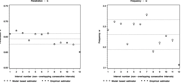
Figure 3 shows time series plots of parameter estimates of

band wcomputed in consecutive non-overlapping inter-vals of length 13 weeks. The plots, in addition, show dot-ted lines representing the overall mean of the estimators and a confidence interval for the mean. The confidence intervals for the mean was computed on the assumption of asymptotic normality of the estimators (for more details see [5]). Note that, for the NBD, the joint parametersb

and w are unique to the joint parameters a and k and thus it is sufficient to consider stationarity of (b, w) when investigating stationarity of (a, k).

The figures indicate that, although the parameter esti-mates forbandware fairly steady, there are two periods for which the estimators significantly differ from one an-other. Note also that, even though the majority of the estimators do not differ significantly, high estimators ofb

tend to have high estimators ofw(i.e. the two estimators seem to be correlated and indeed are correlated).

The methods considered so far only assess adequacy of the one-dimensional marginal distribution of the mixed Poisson process over a fixed analysis period. These meth-ods do not consider the growth of the parameters as the length of the analysis period varies. Figure 4 shows box plots of empirical estimators of penetration and purchase frequency for varying lengths of time window. (For each length of time period, multiple estimators are obtained by taking consecutive non-overlapping analysis periods.) In addition, a solid line is plotted indicating the expected growth of the measure of recurrence based on parame-ter estimates of the mixed Poisson process from a sin-gle period of length 52 weeks. It is clear that the ob-served growth and the model based growth of the mea-sures closely match.

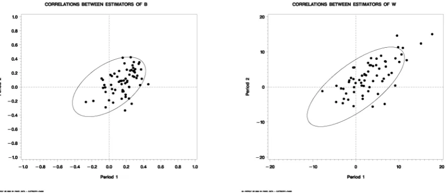
The final method of assessing adequacy of the mixed Poisson process uses the results of [5] in which we de-rive the multivariate asymptotic distributions of statistics and estimators computed over different time intervals us-ing samples observed from mixed Poisson processes. The method of assessing goodness of fit compares the asymp-totic distribution of statistics and estimators (under the assumption that the data are generated from a mixed Poisson process) to the observed distribution of statistics and estimators computed in two different time intervals.

Figure 5 shows, in separate plots, estimators of penetra-tion and purchase frequency computed in two consecutive non-overlapping intervals. The points represent estima-tors obtained from randomly selected sub-groups of the population. In addition, a 95% confidence ellipse is shown which is constructed under the assumption that the data follows a mixed Poisson process and that the estimators are asymptotically normal. The plots again indicate a good fit for the mixed Poisson model.

Figure 1: Assessing adequacy of the MPD (single time interval)

Figure 2: Assessing adequacy of the MPD (multiple time interval)

Figure 4: Assessing adequacy of the MPP using growth curves

Conclusion

The mixed Poisson process has been shown to be an ade-quate model for the modeling of recurrent events in mar-ket research. Numerous methods of assessing adequacy of the mixed Poisson process have been considered. These range from the simplest methods (assessing adequacy of the one-dimensional mixed Poisson distribution) to more complicated methods which take into consideration com-parison of the dynamical behavior the data to the model.

Assessing adequacy of the mixed Poisson processes using methods that take the dynamical behavior of the data into account help examine possible causes of deviation from the model (see e.g. [2]). As a result, it is possible to develop more accurate processes for the modeling of data. For example, it is straightforward to de-seasonalize mixed Poisson processes to homogenous Poisson processes when there are trends in the mean. In the case of panel flow, where individuals have recurrent events that occur ac-cording to a mixed Poisson process for a random period of time, it is possible to extend the standard mixed Pois-son model (see e.g. [6]) to accommodate for panel flow.

References

[1] R. J. Cook and W. Wei. Conditional analysis of mixed poisson processes with baseline counts: implications for trial design and analysis.Biostatistics, 4:479–494, 2003.

[2] A.S.C. Ehrenberg.Repeat-Buying: Facts, Theory and Applications. London: Charles Griffin & Company Ltd.; New York: Oxford University Press., 1988.

[3] Peter S. Fader and Bruce G. S. Hardie. The value of simple models in new product forecasting and customer-base analysis. Appl. Stoch. Models Bus. Ind., 21(4-5):461–473, 2005. ISSN 1524-1904.

[4] J. Grandell. Mixed Poisson processes, volume 77 ofMonographs on Statistics and Applied Probability. Chapman & Hall, London, 1997. ISBN 0-412-78700-8.

[5] V. Savani and A. Zhigljavsky. Asymptotic distribu-tions of statistics and parameter estimates for mixed Poisson processes. J. Statist. Plann. Inference, 137 (12):3990–4002, 2007. ISSN 0378-3758.