Uncertain Decision Tree Inductive Inference
S.M. Fakhrahmad, S. Jafari1Abstract—Induction is the process of reasoning in which General rules are formulated based on limited observations of recurring phenomenal patterns. Decision tree learning is one of the most widely used and practical inductive methods, which represents the results in a tree scheme. Various decision tree algorithms have already been proposed, such as CLS, ID3, Assistant and C4.5. These algorithms suffer from some major shortcomings. In this paper, after discussing the main limitations of the existing methods, we introduce a new decision tree induction algorithm, which overcomes all the problems existing in its counterparts. We also illustrate the advantages and the new features of the proposed method. The experimental results will show the effectiveness of the method in comparison with other methods existing in the literature.
Index Terms—Induction, Classification, Decision Tree Learning, Uncertainty, Outliers
I. INTRODUCTION
Induction or inductive reasoning is a kind of reasoning in which we assert general rules based on limited observations of recurring phenomenal patterns [1,2]. For example, assume that all the people being observed when entering a new city for the first time are short. The conclusion that all the people of the city are short is an
example of induction. Decision tree learning is one of the most widely used and popular inductive methods, which represents the results in a tree scheme [3]. A decision tree is a tree in which each branch node represents a choice between a number of alternatives, and each leaf node represents a classification or decision. A decision tree is
built from a set of data about a number of patterns and represents the decisions or classifications for them. Decision tree learning is best suited to problems in which the training patterns are described in terms of attribute-value pairs, the attribute-values for each attribute range over finitely many fixed possibilities and the target function has discrete values. In other words, we can state the problem of learning decision trees as follows: We have a set of patterns assumed to be correctly categorized into a set of classes. We also have a set of attributes describing the patterns, and each attribute has a finite set of possible values which it can take. We want to use the patterns to learn the structure of a decision tree which will be used to decide the class of an unseen pattern, in the future.
The rest of this paper is organized as follows. Section 2 introduces some existing decision tree learning
1
S.M. Fakhrahmad is with the Department of Computer Engineering, School of Engineering, Islamic Azad University of Shiraz (and PhD student in Shiraz University), Shiraz, Iran
(e-mail: [email protected])
S. Jafari is with the Department of Computer Science & Engineering, School of Engineering, Shiraz University, Shiraz, Iran (e-mail: [email protected])
algorithms. In section 3, our proposed method for decision tree learning and rule extraction is presented and its main advantages are discussed. Experimental results on several benchmark datasets are shown in Section 4. Finally, we give a conclusion at the end of the paper.
II. RELATED WORK
Various decision tree algorithms have already been proposed, such as ID3 [4,5], Assistant and C4.5 [6,7]. These methods have been applied to a wide range of tasks and expert systems including medical diagnosis applications.
This section introduces ID3 and C4.5 methods as two well-known classification algorithms, which represent the classification rules by a decision tree. ID3 is based on a basic algorithm, named CLS (Concept Learning System). Very simply, these algorithms build a decision tree from a fixed set of training patterns. The resulting tree is used to classify future examples. A pattern has some attributes and belongs to a class (like "+" or "-"). The leaf nodes of the decision tree contain the class name whereas a non-leaf node is a decision node. The decision node is an attribute test with each branch (to another decision tree) being a possible value of the attribute. The algorithms use a metric called information gain to help them decide
which attribute goes into a decision node.
A. CLS and ID3
ID3 was originally developed by J. Ross Quinlan at the University of Sydney, in 1975. As mentioned, ID3 is based on the Concept Learning System (CLS) algorithm. Fig. 1 describes the basic CLS algorithm over a set of training patterns S.
Fig. 1. CLS: The basic algorithm for decision tree learning
An important issue in CLS may be the matter of choosing which attribute to test at each node in the tree. In this algorithm, the trainer decides which attribute to select at each node. This is the main difference between CLS and ID3. ID3 improves CLS by adding a heuristic for attribute selection. ID3 searches through the attributes of the training examples and extracts the attribute that best separates the given patterns. If the attribute perfectly classifies the training sets (all negative or all positive)
Algorithm CLS
Input: A set of training pattern S
Output: A Decision tree compatible with all patterns in S
Step 1: If all patterns in S are positive, then create "+" node and halt. Else if all instances in S are negative, create a "-" node and halt. Otherwise select an attribute, A with values v1, ..., vnand create a decision node.
Step 2: Partition the training Patterns in S into subsets S1, S2, ..., Sn according to the values of V.
then ID3 stops; otherwise it recursively operates on the partitioned subsets of each attribute (according to different values an attribute can take) to get the best attribute. The algorithm performs a greedy search, that is, it picks the best attribute and never looks back to reconsider the earlier choices. The details of attribute selection mechanism are as follows.
In ID3, a measure called information gain is defined to
be used to decide which attribute to test at each node.
Information gain is itself calculated using another
measure called entropy, which we first define for the case
of a binary decision problem and then define for the general case.
Given a binary categorization (e.g., "-" and "+"), C, and a set of patterns, S, in which the proportion of examples categorized as "+" by C is p+ and the proportion
of examples categorized as "-" by C is p-, then the entropy
of S is:
(1)
General entropy measure can be defined as follows. Given an arbitrary categorization, C into categories c1, ...,
cn, and a set of examples, S, in which the proportion of
samples in ci is pi, then the entropy of S is:
(2)
When p is very close to zero (meaning that the category
has only a few samples in it), then the log(p) will be a big
negative number, but the p part dominates the calculation,
so the entropy works out to be nearly zero. Since the entropy measures the disorder in the data, this low score is good, as it reflects our desire to reward categories with few examples in. On the other hand, if p is very close to 1
(meaning that the category has most of the samples in), then the log(p) part will be very close to zero, and this
part dominates the calculation, so the overall value gets close to zero. Hence we see that both when the category is nearly - or completely - empty, or when the category nearly - or completely - contains all the examples, the score for the category gets close to zero, which models what we wanted it to. Note that 0*ln(0) is taken to be zero
by convention.
We now return to the problem of trying to decide the best attribute to select for a particular node in a tree. The following measure calculates a numerical value for a given attribute, A, with respect to a set of samples, S. Note that the values of attribute A will range over a set of possibilities which we call Values(A), and that, for a particular value from that set, v, we write Sv for the set of
examples which have value v for attribute A.
The information gain of attribute A, relative to a collection of samples, S, is calculated as:
The information gain of an attribute can be considered
as the expected reduction in entropy caused by knowing the value of attribute A.
ID3 can deal with very large datasets by performing induction on subsets or windows onto the data. For this
purpose, it selects a random subset of the whole set of training instances (called window) and then repeats the following operations until no exceptions left. It uses the induction algorithm to form a rule to explain the selected window, scans all of the training patterns looking for exceptions to the rule, and adds the exceptions to the window.
ID3 is a non-incremental algorithm; meaning that it derives it learns and builds the decision tree from a fixed set of training instances. If a new instance is added to the dataset, it has to restart the construction of the decision tree. An incremental algorithm can revise its current concept definition and update the results, when a new sample is added to the dataset [8,9,10]. The classes created by ID3 are inductive, that is, given a small set of training instances, the specific classes created by ID3 are expected to work for all future instances. The distribution of the unknowns must be the same as the test cases. Induction classes cannot be proven to work in every case since they may classify an infinite number of instances. Note that ID3 and any inductive algorithm may misclassify data.
B. C4.5
C4.5 is another decision tree learning method which makes a number of improvements to the original ID3 algorithm. The main advantages of C4.5 are as follows:
When building a decision tree, C4.5 can deal with datasets that have patterns with unknown attribute values. In such cases, it evaluates the information gain for an attribute by considering just the patterns for which the attribute is defined.
When using a decision tree (for test data), C4.5 classifies patterns having unknown attribute values by estimating the probability of every possible result. These probabilities are computed using the training data. Finally, all possible class labels appear in the classification result each one with a probability.
C4.5 can also deal with the case of attributes with continuous domains by discretization, as follows. Suppose that attribute Ai has a continuous range. It examines the values for this attribute in the training set. Say they are, in increasing order, V1, V2, .., Vm. Then for
each value Vj, j=1,2,..m, it partitions the records into
those that have Ci values up to and including Aj, and
those that have values greater than Vj. For each of these
partitions it computes the gain, or gain ratio, and chooses the partition that maximizes the gain. For example, if the range of values for an attribute is [0..100]. Different partitions can be verified to find the best partition. If the best partition is found to be 80, then the range of this attribute becomes {<=80, >80}. When dealing with continuous attributes, this discretization method (as a preprocessing step) involves a computational overhead.
III. THE PROPOSED ALGORITHM (UD3)
ID3 and other similar methods for decision tree learning have a number of shortcomings. As the main limitations, they do not represent probabilistic rules; for them, there is no more effect for several identical samples than one; they can not deal with inconsistent data and the results are very sensitive to any change in training patterns.
In this section, we introduce our new decision tree induction algorithm UD3, which aims to overcome the problems existing in existing algorithms. There are differences between the proposed method and its counterparts in their approach for tree construction, rule extraction, noise handling and testing the classifier, which will all be discussed.
A. Decision Tree Construction
The procedure we follow to build a decision tree is somewhat similar to which ID3 does. However, it has some major differences. The first difference is that we define and use some binary codes for logical statements and perform binary operations over them to obtain some hidden information, efficiently.
Definition 1.
Binary Code of the decision factor A, for the discrete
value λ (denoted by BCode(A = λ)) is a binary string having a length equal to the number of training samples. Each bit in this string is associated with a sample of the dataset and is set to 1 if A has the value of λ and 0,
otherwise.
In fact, the value of BCode indicates the truth or untruth of a logical statement throughout all samples of a dataset. Based on Definition 1, we can obtain the BCodes for compound logical statements, as follows. Binary Code for a conjunctive compound statement is obtained by performing logical AND operation over the BCodes of all contained statements; that is,
BCode(A1 = λ1 , A2 = λ2 , … , An = λn) = BCode(A1 = λ1) &
BCode(A1 = λ1) & … & BCode(A1 = λ1) (4)
The metric used by our method for attribute selection is the same as ID3. As known, each node in the decision tree stands for an attribute, say A (decision factor) with each branch being a possible value of the attribute, such as λ. Thus, the truth of the branch labeled by λ
throughout the whole data can be implied by the value of BCode(A = λ). While building the decision tree, we measure different BCodes and assign them to their related branches in the tree. Since some inconsistencies may exist in data, the following situation may occur. Assume that we have used all of the attributes as decision nodes in different levels of the tree. When adding the last attribute to the last level of the tree, we can not state a certain class label as a consequent related to that branch. In such cases, we have to specify the class uncertainly by providing the leaf node the error proportion. To do so in an efficient way, we use the following method which specifies the exact place of all exceptional patterns, too.
For a leaf node, say L which can not be certainly specified, we traverse the tree path from the root towards L. Logical AND operation is then performed over all the BCodes visited in the path. The result is a binary string, say BANT in which the 1-bits show the place of samples
whose attributes exactly match the attribute values existing in the path. Since these samples have different class labels, we would rather select one having fewer exceptions as the target class for the rule implied by the path. For this purpose, we build the BCodes for each class label. Let's assume that we have just two classes (- , +)
and the BCodes for them are denoted by B- and B+. As we
aim to find the exceptions of each class as the consequent of the rule, we perform NOT operation on both B- and B+.
Denote the results by B'- and B'+. As the final step, we
perform AND operation on BANT and each of B'- and B'+,
separately. Let's call the resulting bit strings by B rule - and
B rule +. The number of 1-bits in B rule – (B rule +) shows the
number of exceptional samples violating the rule if we select the – (+) as the rule consequent class. One interesting feature of this method is that the indices of 1-bits exactly show the places of the exceptional patterns in the dataset. The class having fewer exceptions is finally selected as the rule consequent to be represented by the leaf node, L. The proportion of 1-bits in its final BCode is used as the error rate of the rule. The described algorithm is presented in Fig. 2.
Fig. 2. The algorithm for assigning a consequent class to a leaf node which can not be certainly defined
Example 2:
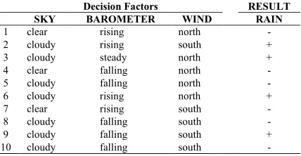
As an example, consider the dataset shown in Fig. 3. This dataset contains a number of training patterns showing whether it had been rainy (or not), sometime in the past. This dataset contains 3 attributes used as decision factors; the sky, the barometer status and the wind direction. Note that there is an inconsistency in the data. That is, the last three patterns show different classes (results), though their attributes are exactly the same. Using the algorithm presented in Fig. 2, this inconsistency is handled while building the decision tree. This is accomplished as follows.
Decision Factors RESULT
SKY BAROMETER WIND RAIN
1 clear rising north -
2 cloudy rising south +
3 cloudy steady north +
4 clear falling north -
5 cloudy falling north -
6 cloudy rising north +
7 clear rising south -
8 cloudy falling south -
9 cloudy falling south +
10 cloudy falling south -
[image:3.612.326.540.550.661.2]
Fig. 3. An example dataset containing inconsistencies
Step1:
BCode(Sky = 'Cloudy') = 0110110111 BCode(Barometer= 'Falling') = 0001100111 BCode(Wind = 'South') = 0101001111
Algorithm FindRuleConsequent
Input: A decision tree T with an uncertain leaf node L Output: The class label for L, provided by an error rate
Step1: Traverse the path from the root towards L,
Perform AND operation on all BCodes in the path; Denote the result by BANT.
Step2: Build BCodes for both classes; Denote the results by B- and B+.
Step3: Perform NOT operation on B- and B+; Denote the results by B-' and B'+.
Step4: Use AND operation between BANTand each of B'- and B'+; Denote the results by Brule- and Brule +.
Step5: For Brule - and Brule + , count the no. of 1-bits (e- and e+) and
select the string containing fewer 1-bits.
Compute the proportion of 1-bits in the selected string as the error rate.
BANT = BCode(Sky = 'Cloudy' , Barometer= 'Falling' ,
Wind = 'South') =
0110110111 & 0001100111 & 0101001111 = 0000000111
Step2:
B- = BCode(Rain = '-') = 1001101101
B+ = BCode(Rain = '+') = 0110010010
Step3:
B-' = 0110010010
B+' = 1001101101
Step4:
Brule - = BANT & B-' = 0000000111 & 0110010010 =
0000000010, e- = 1
Brule + = BANT & B+' = 0000000111& 1001101101=
0000000101, e+ = 2
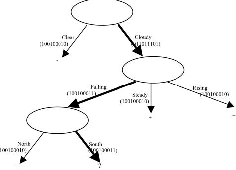
[image:4.612.63.301.338.509.2]The purpose of the above process is to find the proper alternative class label for the "?", shown in Fig. 4. The final bit strings imply that if we replace "?" by "+", the resulting rule will include two exceptions (patterns no. 8 and 10), while selecting "-" will lead to just one exception for the rule (pattern no. 9).
Fig. 4. The Decision tree built for the dataset shown in Fig. 3
A1) Deriving Rule Set
As illustrated before, in ID3, each path from the root of the decision tree to a leaf node will be represented by an if-then rule. That is, the number of rules is equal to the number of leaf nodes of the decision tree. In the proposed method, the rules are extracted from different branches of the tree. However, it has some major differences. The first difference is that in the proposed scheme, we may have uncertain rules (which have exceptions in the training data) and thus a certainty factor (CF) should be defined for them.
To evaluate a rule, we use two well-known metrics, namely, confidence and Support, which are the major
measures in the mining of frequent patterns and association rules [11,12]. The support of a rule X → Y is
defined as the proportion of patterns in the dataset satisfying X and Y, simultaneously. The confidence of a rule X → Y is defined as support(X ∩ Y )/support(X),
i.e., the fraction of all patterns satisfying X, which satisfy Y as well. Since these two factors are important for a rule to be considered as an interesting rule, we use both of them to define a certainty factor for generated rules (CF), as shown in (5).
CF(rule) = Confidence(rule)*Support(rule) (5)
The values of Confidence and Support can also be easily computed from the resulting bit strings. If the class "-" ("+") has been selected for the rule consequent, the support value of the rule can be obtained from the proportion of 1-bits in Brule – (Brule +), which shows the
fraction of patterns that satisfy both the premise and the consequent of the rule.
Support(rule) = e* / (no. of patterns) (6)
where e* stands for e- or e+, based on the rule's
consequent.
Beside their main meaning, e- and e+ imply another
concept, too. e- (e+) is the no. of patterns that violate the
rule whose consequent is "-" ("+"). From another viewpoint, we can say that e- (e+) is the no. of patterns
which satisfy the rule whose consequent is "+" ("-"). Thus, (e- + e+) is the no. of all patterns that satisfy the
premise of the rule, without any attention to their class labels, whereas max(e- , e+) indicates the no. of patterns
that satisfy the whole rule. The Confidence of the rule can be obtained from equation (7).
Confidence(rule) = max(e- , e+) / (e- + e+) (7)
As an example, the certainty factor of the rule discussed in Example 2 can be computed as follows:
e- = 1, e- = 2
Confidence(rule) = max(2,1)/(2+1) = 2/3 Support(rule) = 2/10 = 0.2
CF(rule) = 2/3 * 0.2 = 4/30 = 0.13,
and the resulting rule is presented in the following format: If (Sky = 'Cloudy' AND Barometer= 'Falling' AND Wind = 'South') Then It will not rain (-), CF = 0.13
Now, assume that a decision tree has been built for a dataset containing a large number of attributes. Also, assume that the tree includes many long branches from the root to the leaf nodes, i.e., long if-then rules. In this situation, we may prefer to have rules which have shorter lengths, even if they have smaller CF values. For this purpose, we can select any top-down path, which can be between any two nodes within the tree. The selected path represents the antecedent part of a rule, whose consequent should be determined. We make a small variation to the algorithm presented in Fig. 2 and then follow it to specify the consequent of the rule. The mere change occurs in Step1 of the algorithm, where we traversed the whole path from the root to a leaf node. In the current case, we traverse the selected path and measure BANT just from the
combination of BCodes located within the path.
Example 3:
Consider that the decision tree shown in Fig. 4 has been constructed. Assume that we are just interested in rules having not more than 2 antecedents. The process of rule
BAROMETE R SKY
WIND
Clear Cloudy
Falling
Steady
Rising
North South
-+ ?
(100100010) (011011101)
(100100011)
(100100010)
(100100010)
(100100010) (100100011)
extraction from all branches of the tree can be accomplished straightforward, except the branch which is shown in more significance. This branch has 3 decision factors (and 3 BCodes). Any two of these decision factors can be selected to form a two-antecedent rule. To do so, we traverse the branch and perform AND operation over the BCodes of only two of the decision factors, as we want them to be present in the rule's premise. Selecting
SKY and BAROMETER, for example, the process of rule
extraction will be as follows:
BCode(Sky = 'Cloudy') = 0110110111 BCode(Barometer= 'Falling') = 0001100111
BANT = BCode(Sky = 'Cloudy' , Barometer= 'Falling') =
0110110111 & 0001100111 = 0000100111
B- = BCode(Rain = '-') = 1001101101
B+ = BCode(Rain = '+') = 0110010010
B-' = 0110010010
B+' = 1001101101
Brule - = BANT & B-' = 0000100111 & 0110010010 =
0000000010, e- = 1
Brule + = BANT & B+' = 0000100111 & 1001101101=
0000100101, e+ = 3
The same as the last example, the class "-" is selected again:
If (Sky = 'Cloudy' AND Barometer= 'Falling' AND Wind = 'South') Then It will not rain (-)
Confidence(rule) = max(3,1)/(3+1) = 3/4 Support(rule) = 3/10 = 0.3
CF(rule) = 3/4 * 0.3 = 9/40 = 0.225
A2) Handling Noisy Data
Assuming that there are no inconsistencies in the data (when two examples have exactly the same values for the attributes, but are categorized differently), it is obvious that we can always construct a decision tree to correctly decide for the training cases with 100% accuracy. All we have to do is make sure every situation is catered for down some branch of the decision tree. Of course, 100% accuracy may indicate overfitting. In ID3, if some noisy patterns exist in the dataset, they will be the main cause for overfitting. This is because the decision tree is constructed according to the attribute values of the decision tree. Noisy patterns (outliers) will affect on the structure of the decision tree. In our proposed method, in order to decrease the effect of outliers on the decision tree structure, we follow the following strategy. Consider a dataset structurally similar to the dataset shown in Fig. 3, which contains 1000 training patterns. Assume that the attribute SKY is selected to be located as the root of the
decision tree (the same as Fig. 4). One of the possible values for this attribute is "Clear" which will be
represented by a branch from the root. The same as ID3, we compute the values of p+ and p-, for patterns in which
the value of SKY is "Clear". In ID3 the extension of a
branch will stop only if one of these two values (p+ and p-) is 1 and the other is 0. This means that the
consequent class can now be stated, with certainty. However, in this example, assume that just one of the patterns (in which the value of SKY is "Clear") has the "-"
class label, while all others are from the "+" class. This
pattern is more likely to be an outlier. Thus, we ignore such exceptional patterns while building the decision tree. In general, when there is a high gap between the values of p+ and p- (p+<<p- or p-<<p+) we assume the greater value
to be 1 and the other to be 0. In practice, we define a minimum threshold called ρ for p+/p- or p-/p+. If any of
these proportions is less than ρ, we stop extending of the branch and assign it a consequent class according to the majority. If a proper value is assigned to ρ, this strategy will be very effective for avoiding overfitting. This will be shown experimentally, in Section 4.
A3) Testing the Classifier
In order to classify a test pattern, it is compared with every rule within the rule base, to find the rule which is compatible to be fired. However, in some cases, we may find more than one rules which are satisfied by the pattern attribute values. If all of them have the same consequent, there will be no ambiguity for the pattern's class. Otherwise, suppose that we are encountered two (in case of binary categorization) or n (in case of n-ary categorization) groups of rules, where each group consists of rules showing a different class label. For each group, we compute the average of all CF values belonging to the contained rules. Finally, the rules having the maximum value for their CFs, are used to classify the test sample.
IV. EXPERIMENTAL RESULTS
In order to assess the performance of the proposed scheme over some real-life data, we used the data sets shown in Table I available from UCI ML repository, most of which are medical datasets. For rulebase construction, we used 10CV technique which is a case of n-fold cross validation. In this experiment, we compared our proposed method with two other inductive rule-based methods, ID3 and C4.5, which were introduced in Section 2. Since the datasets contain continuous numeric data, as a preprocessing step, each continuous attribute was discretized by partitioning the domain interval of the attribute into five equi-width intervals.
Table I. Some statistics of the datasets used in our computer simulations
Data set Number of attributes
Number of patterns Number of classes
Iris 4 150 3
Wine 13 178 3
Thyroid 5 215 3
Sonar 60 208 2
Bupa 6 345 2
Pima 8 768 2
Glass 9 214 6
In the implementation of the proposed method, all strategies discussed in Section 3 were attended in order to optimize the accuracy, the efficiency and the interpretability. For a dataset containing n attributes, we
restricted the rules to have not more than n/2 antecedent
conditions. We tested three different values for the ρ (the minimum threshold of p+/p-, as discussed in Section
3.1.2) to evaluate the effect of using this threshold and the proper value it should be assigned to.
The results of the other two methods, ID3 and C4.5 on different datasets are also shown in this table.
Although ID3 always gets the accuracy of 100% over the training data, we can see in Table I that among the three methods, it has the least values of the accuracy over the test data. This narrates from the problem of overfitting in ID3. C4.5 has better accuracies compared to ID3, which can be due to the principal variations it has made in its algorithm.
Comparing the results obtained from running of the proposed method using different values of ρ implies that using this strategy (using a threshold for p+/p-) will have
positive effect on the generalization accuracy and in order to avoid overfitting. However, it should be selected carefully. If the value of ρ is very small (very close to zero), it does not have any effect, since according to the no. of patterns, this proportion may represent even less than 1 pattern out of the whole! On the other hand, if a large value is given to ρ, it may have some negative effect on the classifier's accuracy. In this case, the accuracy may decrease on both the training and the test data.
As shown in Table II, in most cases, when ρ has a relative proper value, the proposed classifier results in better classification rates, compared to the results of C4.5.
V. CONCLUSION
In this paper, we proposed a new decision tree induction algorithm, called UD3. The basis of this method is similar to other decision tree algorithms, such as ID3 and C4.5. However it has some valuable advantages to its counterparts. In order to improve efficiency, the proposed scheme maps some important information into special bit strings and makes use of the speed of logical operations over them during the induction process. On the other hand, the method can deal with inconsistencies in data and also it provides uncertainty. A very important feature of the method which helps much to avoid overfitting, is its flexibility in decision tree making and rule extraction from the tree. Unlike ID3, it does not try to completely satisfy all the training patterns with the constructed tree. In order to obtain a good generalization accuracy, it avoids generating rules for patterns that seem very exceptional, since they are likely to be outliers. For rule extraction from the constructed tree, we are able to choose any path within the tree (not essentially a full path from the root to a leaf node) to be represented as an if-then rule. Every generated rule is provided by a certainty
factor (CF) which is easily calculated and can be used as a metric for rule selection when testing the system.
In order to evaluate the classification ability of the proposed method over some real-life data, we used the some benchmark datasets available from UCI ML repository, most of which are medical datasets. The proposed method was compared with two other inductive rule-based methods, ID3 and C4.5, as two well-known methods. Our method uses a parameter ρ, while constructing the decision tree. The experimental results showed that when a proper value is assigned to ρ, the algorithm will result in better generalization ability, in comparison with ID3 and C4.5.
REFERENCES
[1] John, H., et al., Induction: Processes of Inference, Learning and Discovery, MIT Press, 1986.
[2] S. Muggleton, Inductive Acquisition of Expert Knowledge, Addison-Wesley, 1990.
[3] Breiman, Friedman, Olshen, Stone, Classification and Decision Trees, Wadsworth, 1984.
[4] Andrew Colin, Building Decision Trees with the ID3 Algorithm, Dr. Dobbs Journal, June 1996
[5] P.H., Winston, Excellent introduction to ID3 and its use in building decision trees and rule sets from them, Artificial Intelligence, Third Edition, Addison-Wesley, 1992.
[6] J. Ross Quinlan, Morgan Kaufmann,"C4.5 Programs for Machine Learning", 1993.
[7] Lynn Monson, "Algorithm Alley Column: C4.5", Dr. Dobbs Journal, Jan 1997.
[8] Paul E. Utgoff and Carla E. Brodley, 'An Incremental Method for Finding Multivariate Splits for Decision Trees', Machine Learning: Proceedings of the Seventh International Conference,
pp.58, 1990.
[9] Paul E. Utgoff, "Incremental Induction of Decision Trees", Kluwer Academic Publishers, 1989.
[10] S.M. Fakhrahmad , M.H. Sadreddini and M. Zolghadri Jahromi, "IQPI: An incremental system for answering imprecise queries using approximate dependencies and concept similarities", Accepted for publication in International Journal of Computer Science (IJCS), Vol 34, Issue 2, 185-191 (Dec 2007).
[11] S.M. Fakhrahmad, M.H. Sadreddini and M. Zolghadri Jahromi, "Mining Frequent Itemsets in Large Data Warehouses: A Novel Approach Proposed for Sparse Data Sets", In Proc. of: IDEAL2007, Springer, 16-19 Dec 2007, Birmingham, UK, pp. 517-524.
[12] H. Ishibuchi, T. Yamamoto, Fuzzy rule selection by multi-objective genetic local search algorithms and rule evaluation measures in data mining, Fuzzy Sets and Systems, Vol 141, Issue 1, 59-88 (2004).
[13] S.M. Fakhrahmad and M. Zolghadri Jahromi, "Constructing Accurate Fuzzy Classification Systems: A New Approach Using Weighted Fuzzy Rules", 4th International Conference (IEEE) on Computer Graphics, Imaging and Visualization, (CGIV07), Bangkok, Thailand, 15-17 August 2007, pp. 408-413.
[14] Q. Yang, T. Li, K. Wang, Building association rule based sequential classifiers for web document prediction, Journal of Data Mining and Knowledge Discovery, 8(3) (2004) 253-273.
[15] H. Ishibuchi, T. Yamamoto, Fuzzy rule selection by multi-objective genetic local search algorithms and rule evaluation measures in data mining, Fuzzy Sets and Systems 141 (1) (2004) 59-88.
[16] L. Sánchez, I. Couso, J. A. Corrales, O. Cordón, M. J. Del Jesus, F. Herrera, Combining GP operators with SA search to evolve fuzzyrule based classifiers, Information Sciences 136 (1-4) (2001) 175-191.
[image:6.612.66.295.119.229.2][17] A. Chatterjee and P. Siarry, A PSO-aided neuro-fuzzy classifier employing linguistic hedge concepts, Expert Systems with Applications 33 (4) (2007) 1097-1109.
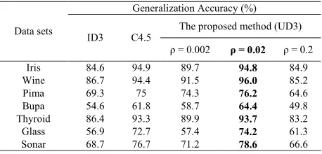
Table II. Classification Accuracies of the proposed method using different values for ρ (minimum threshold for p+/p-) in
comparison with ID3 and C4.5 for data sets of Table I
Generalization Accuracy (%) The proposed method (UD3) Data sets
ID3 C4.5
ρ = 0.002 ρ = 0.02 ρ = 0.2
Iris 84.6 94.9 89.7 94.8 84.9
Wine 86.7 94.4 91.5 96.0 85.2
Pima 69.3 75 74.3 76.2 64.6
Bupa 54.6 61.8 58.7 64.4 49.8
Thyroid 86.4 93.3 89.9 93.7 83.2
Glass 56.9 72.7 57.4 74.2 61.3