Journey Time Estimation Using Route Profiles
Shane Bouchier
A dissertation submitted to the University of Dublin, in partial fulfillment of the requirements for the degree of
Master of Science in Computer Science
Declaration
I declare that the work described in this dissertation is, except where otherwise stated, entirely my own work and has not been submitted as an exercise for a degree at this or any other university.
Signed: ___________________ Shane Bouchier
Permission to lend and/or copy
I agree that Trinity College Library may lend or copy this dissertation upon request.
Signed:________________ Shane Bouchier
Acknowledgements
Abstract
Estimating journey times is of increasing importance in the modern world for the fulfilment of social and business occasions. Probably the most variable journey times are the times experienced when using a road network. Intelligent Transportation Systems (ITS) are used to address this problem to estimate journey times for interested authorities and commuters.
This dissertation presents the design, implementation and evaluation of a tool that is used to generate route profiles for use in the ITS domain. The tool is biased for use on the inter-urban national primary routes in the Republic of Ireland. This ubiquitous computing project allows journey times to be generated using a set of probe vehicles. The probe vehicles are tracked using Global Positioning System (GPS). Journey times are tagged with context data such as the prevailing weather conditions during the time the GPS reading was made.
To accomplish the above goals, a Geographic Information System (GIS) application was developed in order to process GPS and weather data to produce contextualised journey records. These historical records are stored in a database and queried by a web server to deliver records to the road management tool or traveller information system.
Contents
1. INTRODUCTION……...1
1.1. Background ...1
1.2. Previous Work (JETS) ...1
1.3. Route Profiles ...2
1.4. Project Goals...3
1.5. Project Scope ...3
2. STATE OF THE ART ...4
2.1. Journey Time Estimation using Inductive Loops ...4
2.2. Journey Time Estimation using Infra-red...5
2.3. Journey Time Estimation using Road Side Transmitters ...6
2.4. Journey Time Estimation using GPS ...6
2.5. Journey Time Estimation and Weather Impacts ...7
3. BACKGROUND RESEARCH...8
3.1. Weather data available ...8
3.2. Weather Contexts...9
3.3. The Irish Road Weather Information System ...12
3.4. Review of Open Source GIS Systems...16
3.4.1. GRASS (Geographic Resource Analysis Support System) ...16
3.4.2. JUMP (Java Unified Mapping Platform)...18
3.4.3. MapServer ...19
3.4.4. GeoTools ...20
3.4.5. OpenMap ...21
3.5. Evaluation of Open Source GIS Systems ...22
3.5.1. GRASS ...22
3.5.2. JUMP...23
3.5.3. MapServer ...23
3.5.4. GeoTools ...23
3.5.5. OpenMap ...24
3.5.6. GIS Evaluation Conclusion ...25
4. DESIGN……… ...26
4.3. Context Acquisition ...28
4.4. Context Application ...29
4.5. Traveller Information System...31
5. IMPLEMENTATION ...32
5.1. Pre-Processing of Map Data ...32
5.2. Coordinate Conversion...34
5.2.1. Introduction...34
5.2.2. The Irish Grid Reference System ...34
5.2.3. The Modified Airy Ellipsoid...34
5.2.4. The Transverse Mercator...35
5.2.5. Coordinate Conversion...36
5.2.6. Evaluation of Coordinate Conversion ...37
5.2.7. A New Coordinate System ...38
5.3. GPS Data Processing...38
5.4. Map-Matching………...42
5.5. Context Data Processing ...43
5.6. Web Interface………. ...44
6. EVALUATION…….. ...46
6.1. Evaluation of GPS Data ...46
6.2. Evaluation of Weather Data ...47
6.3. Evaluation of Route Profiles...48
7. CONCLUSIONS…….. ...49
7.1. Goals Achieved...49
7.2. Recommendations for Future Work...49
8. APPENDIX………. ...51
Table of Figures
Fig 2.1 Road side cameras and intra-red transmitters………... 6
Fig 3.1 Drivers Response to Weather Conditions when Advised in Idaho….. 10
Fig 3.2 Force 4 to 6 of the Beaufort scale………. 10
Fig 3.3 IceView………. 12
Fig 3.4 ROSA Ice Warning Station……….. 13
Fig 3.5 DRS511 Road/Runway Sensor………. 13
Fig 3.6 The principle of the optical “eye”……… 14
Fig 3.7 WA15, complete with anemometer and wind vane……….. 15
Fig 3.8 Sample Data Set evaluated using GeoTools………. 25
Fig 4.1 Deployment Diagram………... 26
Fig 4.2 Town Schema………... 27
Fig 4.3 Road segment schema……….. 27
Fig 4.4 Journey time data schema………. 27
Fig 4.5 Coordinate Conversion………. 28
Fig 4.6 Weather data schema……… 29
Fig 4.7 Context Acquisition……….. 29
Fig 4.8 Sensor Data Schema………. 30
Fig 4.9 Context Application……….. 30
Fig 4.10 A hierarchical way to represent context………... 30
Fig 4.11 Architecture diagram for the journey time estimation system………. 31
Fig 5.1 Pre-Processing Class Diagram………. 32
Fig 5.2 Motivation for Pre-Processing……….. 33
Fig 5.3 Airy Modified is a better fitting for Ireland rather than GRS80……... 35
Fig 5.4 Transverse Mercator Projection onto a Plane Grid……….. 35
Fig 5.5 Goal of the Coordinate Conversion Module……… 36
Fig 5.6 Irish Parameters to Transverse Mercator……….. 36
Fig 5.7 OSi Computations of E and N from Φ and λ……… 37
Fig 5.8 GeoTools Computations of E and N from Φ and λ……….. 37
Fig 5.9 Sample GPS Data………. 39
Fig 5.10 GPS Processing Class Diagram……… 39
Fig 5.11 towns Table and Sample Data……….. 39
Fig 5.15 Road Buffers Illustration……….. 43
Fig 5.16 Sensor Definition Example………... 43
Fig 5.17 Weather Processing Class Diagram……….. 44
Fig 5.18 Servlet's definition of time periods………... 44
Fig 5.19 Servlet Class Diagram……….. 45
Fig 6.1 Journey time data generated using a fleet of probe vehicles………… 46
Fig 6.2 Aggregated weather data from a roadside weather station…………... 48
Fig 8.1 Web Front End………. 51
1. INTRODUCTION
1.1. Background
The volume of traffic on our roads has increased significantly and more and more people are now using cars as their primary transport means. This has resulted in road networks pushed to their capacity as commuters rush to their place of work/leisure or intended destination. Growing economies across the world means that there is also an increase in commercial traffic. Due to increased road capacity, distance is no longer used for profiling routes in terms of journey time estimation, as time taken is more important information for travellers. Increased volumes of traffic on our roads lead to increased delays as some roads cannot cater for increased volumes so average journey times for particular routes increases.
However, increased traffic volumes are not the only element that effects journey times. Weather has a significant influence on journey times. Heavy rain, snow, ice can
increase journey times. Road events such as road works, accidents, pop concerts, etc, also reduce roadway capacity.
Road management authorities are under pressure to provide a better level of service. Authorities need accurate journey time estimates, so that road segments which have a low customer satisfaction can be pin pointed by the authorities. Road segments in this project refer to the national primary routes between adjacent towns. To address this problem a journey time estimator is required. Traditionally this was done by moving car surveys where an observer would note times at various point along a journey. Lots of research has been done in the past to predict journey times given the speed of a vehicle between two designated points. The designated points would be inductive loops or infra-red detectors.
1.2. Previous Work (JETS)
Estimation System (JETS) prototype for vehicular traffic that is based on the use of GPS data provided by a number of third party information providers. The Distributed Systems Group at Trinity College Dublin completed this work during 2002.
This prototype was developed using C, Java and MapBasic. The prototype processes GPS data only and generates journey times based on these readings. The production of contextualised journey times is a feature that the ITS domain needs. This spawned the initiative to re-architect the above prototype to include support for tagging journey times with context data.
The use of MapBasic or other client-server geographic information systems for the above prototype revealed that a GIS with APIs would be a more flexible solution and less clumsy. The use of a GIS with a Java API would facilitate the portability of the new GIS application and allow it to be less architecturally constrained.
1.3. Route Profiles
Route Profiles are a set of routes that are organised by descriptions of the routes. Routes may be described by:
• Physical Features such as location, curvature, altitude, slope, etc [1]
• Dangers along the route
• Proximity to venues that may cause traffic disruption
• Weather conditions along the route
As manual collection of this data is unfeasible, sensors may be deployed along a route network to collect information that would help to build route profiles.
In the context of journey time estimation, it is important to build route profiles based on weather conditions along a route. The fixed sensors available for this project are
1.4. Project Goals
• Development of a Geographic Information System (GIS) to process Global
Positioning System (GPS) data and other sensor data to produce contextualised data that can be used to manage transport infrastructure in the Intelligent Transportation Systems (ITS) domain.
• The goal of the project is not to predict journey times but rather to estimate journey times based on historical data collected from previous journeys made on particular routes.
• The set of relevant context data that can be tagged to journey times includes
details on weather and road events.
1.5. Project Scope
The GIS application produces route profiles of inter-urban national primary routes in Ireland. The project does not cover journey time estimation for urban routes. The current implementation determines journey times from processing GPS data and does not have support for processing journey time data from, for example, inductive loops or infra-red sensors.
Road management authorities have criteria for whether or not journey times are adequate for road segments. This adequacy equates to a providing a minimum inter-urban journey speed. It is not in the scope of this project to estimate journey times by providing the average speed of a vehicle along a road segment.
2. STATE OF THE ART
Despite the advancements in Intelligent Transportation Systems, the most widely used method of collecting traffic information and journey times are inductance loops. The following sections describe papers or reports that describe different methods used to estimate journey times.
Estimating Travel Times of Field Engineers [2]
British Telecom has a lot of field engineers out on sites and travelling between sites. In order to produce reliable schedules, British Telecom management needs estimates of how long it takes for an engineer to get from one site to another, i.e. inter-job time. A generic platform called Intelligent Travel Time Estimation and Management System (ITEMS) was developed for British Telecom. The Travel Time Estimation System (TTE) receives job data every night and updates its prediction model accordingly. Using the TTE, British Telecom found that it improved their travel time estimates by 10%.
2.1. Journey Time Estimation using Inductive Loops
Journey time estimation using single inductive loop detectors on non-signalised links [3]
This paper describes two techniques for estimating journey times and makes
comparisons between the two. One technique is a mechanistic approach and the other uses a neural network approach. Both techniques use single inductive loop detectors to collect the data. The mechanistic approach estimates journey times every thirty seconds based on the time taken for the vehicle to traverse over the pair of detectors. The neural network approach uses this data, plus average time-gap between the vehicles and percentage occupancy derived from the inductive loops. This data is presented to a neural network for training.
Day-to-Day Travel Time Trends and Travel Time Prediction from Loop Detector Data [4]
This paper presents an approach to estimate journey times given data from single loop detectors and historical travel time information. The current traffic state proved to be a good estimator for the near future (up to twenty minutes). The historical information was more useful for longer range predications. This system relies strictly on detector data. Parameters such as major events, incidents or weather conditions were not included in the model. The paper concludes that the prediction model only works for short stretches of roadway (up to 15km).
2.2. Journey Time Estimation using Infra-red
Travel Time Generation and Dissemination within Centrico [5]
France has invested considerably in traveller information systems to provide travel times to motorists. French motorway company SAPN (Société Des Autoroutes Paris-Normandie) generates travel times from existing spot speed detectors on the A13 motorway northwest of Paris. Accurate journey time information is required on this motorway given its high traffic volume. The company performed several studies and concluded that accurate journey times could be estimated from spot speed
measurements; this also allowed the company to make use of present traffic monitoring investments. The spot speed measurements were made using infra-red. Using the data from the infra-red detectors and existing inductance loops the SAPN system estimates journey times using a multiple linear regression model. The Travel time system then provides information to the SSA (Système de Supervision Autoroutier) which transmits travel times to drivers using FM radio, variable message signs, WAP and the company internet site.
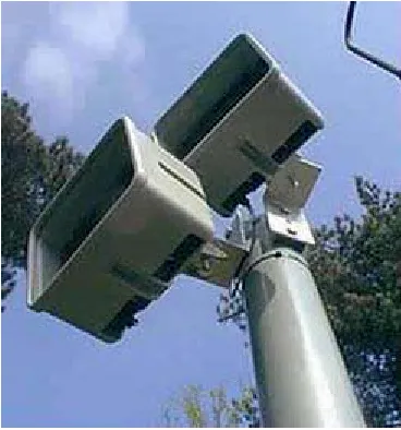
Golden River Traffic [6]
Fig 2.1 Road side cameras and intra-red transmitters (www.goldenriver.com)
2.3. Journey Time Estimation using Road Side
Transmitters
Dynamic Travel Time Prediction with Real-Time and Historic Data [7]
In this paper, data was collected using road side transmitters (RST). When a vehicle (equipped with an electronic pass) passes a RST, the RST radiates a signal to
interrogate the vehicle’s tag. The vehicle responds by transmitting its tag id. Each RST receives information like tag id, detection time, location and lane position. The
information is then recorded and sent to the Operations Information Center (OIC) where it is stored in a database. To ensure that the vehicles make sufficient progress, travel time between two particular readers is calculated and is compared with the average travel time of its leading vehicles travelling on the same segment and in the same time interval.
2.4. Journey Time Estimation using GPS
Journey Time Analysis From GPS based tracking systems [8]
GPS data is matched with a GIS application to determine the journey times. The system was evaluated using people to survey the traffic and when compared with the journey times generated from the GIS application, the results show a 95% confidence interval.
2.5. Journey Time Estimation and Weather Impacts
Analysis of Weather Impacts on Traffic Flow in Metropolitan Washington DC [9]
The Federal Highway Administration (FHWA) has been sponsoring research into the impacts of weather on surface transportation. Some of the research involves
investigating the travel delay associated with the influence of weather. This paper describes two methods used to approximate the delay given the influence of adverse weather.
The first method was regression analysis using surface observations from three Washington area airports. The hourly weather observations from the airports were organised into discrete elements such as Sky Cover, Surface Visibility, Wind Speed, etc. These elements were then converted into categories so that the data could be used later for processing. The travel time data and the weather data was combined by assigning travel times to a weather observation if the travel time lies within thirty minutes before or after the weather observation was made. Since the weather
observations did not correlate with specific road segments, regression models were used to predict travel times on the road segments.
3. BACKGROUND RESEARCH
Weather events such as precipitation, fog, high winds, high water, and extreme temperatures (e.g. ice formation / tar melting) reduce roadway capacity. These events can cause lower traffic speeds, affect traffic volume and increase delay. In poor road weather conditions, arterial traffic volumes can decline by six to thirty percent, depending on the time of day [10].
Weather impacts journey times in many ways:-
• Weather impacts driver behaviour. e.g., In the case of reduced visibility, headway (spacing between vehicles) is naturally increased by virtue of drivers slowing down for safety [10].
• Weather influences which mode of transport the public choose. For example, if
there is heavy rain in the morning, instead of usually walking, one may take the car.
• Vehicles perform differently depending on the weather conditions, e.g., wet
conditions decrease tyre grip and strong wind increases (if travelling against wind direction) wind resistance.
• Weather impacts road safety. Severe winds can cause fallen trees, ice can cause
skids and the sun can cause dazzle. Accidents and infrastructural damage influence journey times.
3.1. Weather data available
The National Roads Authority of Ireland (NRA) has fifty two strategically placed weather stations, called Road Weather Information Systems (RWIS). The following weather data is available from these stations. This data was derived from weather records supplied by the NRA and researching the details of the equipment in use.
• Air Temperature (°C)
• Road Surface Temperature (°C)
o Dry
o Moist
o Wet
o Treated
o Moist & Treated
o Wet & Treated
o Frost
o Snow
o Icy
• Relative Humidity (%)
• Wind Speed (mph)
• Wind Direction (degrees)
• Precipitation State
o No Recent Rainfall
o Light Rainfall
o Medium Rainfall
o Heavy Rainfall
o Snow
• Dew Point Temperature (°C)
• Freezing Point Temperature (°C)
• Five Centimetre Depth Temperature (°C)
• Thirty Centimetre Depth Temperature (°C)
3.2. Weather Contexts
3.2.1. Wind
The Idaho Department of Transportation has a motorist warning system. The system was evaluated between 1993 and 2000 to access changes in driver behaviour when warned of high winds (> 20mph). When drivers were confronted with high winds and
moderate to heavy precipitation without a warning system, average speeds were 12 per
cent lower than average when there were no high winds. [12]
Road Weather Conditions Speed without Advisories
Speed with Advisories
Speed Reduction due to Advisories
High Winds (over 32.2 kph or 20 mph) 88.1 kph (54.8 mph) 68.0 kph (42.3 mph) 23 percent
High Winds & Precipitation 75.6 kph (47.0 mph) 66.2 kph (41.2 mph) 12 percent
[image:19.595.89.562.197.335.2]High Winds & Snow-Covered Pavement 87.9 kph (54.7 mph) 56.9 kph (35.4 mph) 35 percent
Fig 3.1 Drivers Response to Weather Conditions when Advised in Idaho
Research done in Kent University Ohio [13] determined that wind speeds of about 95 mph may tip over high profile vehicles or buses. At a wind speed of 125 mph, fewer than 10% of cars, vans and pick-ups are tipped over.
Given these findings, wind context in this project will be divided into two contexts:
! moderate or no wind (<20 mph)
! high wind (≥ 20 mph)
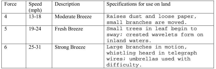
The Beaufort wind scale for use on land describes the dangers of wind speed:
Force Speed (mph)
Description Specifications for use on land
4 13-18 Moderate Breeze Raises dust and loose paper,
small branches are moved.
5 19-24 Fresh Breeze Small trees in leaf begin to
sway; crested wavelets form on inland waters.
6 25-31 Strong Breeze Large branches in motion,
whistling heard in telegraph wires; umbrellas used with
difficulty.
[image:19.595.81.523.577.720.2]3.2.2. Precipitation
All forms of precipitation can impact traffic flow.Precipitation reduces visibility, vehicle performance and roadway capacity [10]. A detailed analysis using Doppler radar data indicated that, during peak periods, travel time increases by roughly twenty four percent with precipitation [9].
This project will use the following precipitation contexts:
! No Rain (Precipitation State: No Recent Rainfall, Light Rainfall)
! Rain (Precipitation State: Medium Rainfall, Heavy Rainfall)
! Snow (Precipitation State: Snow)
These precipitation contexts are biased towards the Irish climate.
3.2.3. Pavement
Condition
It is important to differentiate between precipitation and pavement condition. At the Ministere de l’Equipement et des Transports in France a statistical analysis was performed of precipitation and state of the road. This study determined that during January, February and March, 52.4% of the road weather data received indicates a moist road surface (and 6.4% wet). On the other hand, the road weather data received indicates precipitation (rain/snow) for only 7.6% of the time [14].
This project will use three road state contexts:
! Dry (Road State: Dry)
! Wet (Road State: Moist, Wet)
3.3. The Irish Road Weather Information System
The road ice monitoring system used by the NRA is called IceCast [15]. This allows
local authorities to predict (within certain accuracy) whether segments of the road network are likely to be affected by snow or ice conditions. Road monitoring stations are strategically positioned throughout the road network. The data is collected and relayed to Met Éireann (via GPRS), who inform the local authorities whether road treatment is needed, e.g., gritting.
IceCast Traffic Safety Solutions are supplied by Vaisala, a Finnish company who are the World’s leading supplier of meteorological instruments and services to transport professionals in more than 100 countries. IceCast integrates data from Vaisala ROSA weather stations as well as local forecast data and thermal maps to determine [16]:
• The need to treat the road network
• Which roads to treat
• The time to treat
• The optimum rate of the spread of salt
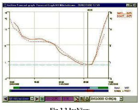
[image:21.595.186.416.526.708.2]IceView is used by Met Éireann [17] to display the ROSA weather station and forecast data. Graphs, maps and tabular displays of current, historic and forecast data are displayed.
Fig 3.3 IceView
ROSA Ice Warning Stations provide real-time weather and pavement data to
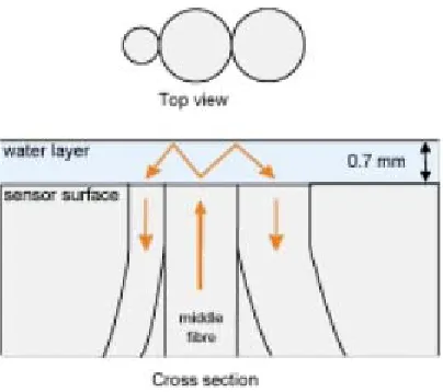
[image:22.595.214.389.175.401.2]immediately inform decision-makers of ice, snow and low visibility. The station reports on surface and ground temperature, water layer thickness, air temperature, humidity, dewpoint and precipitation, and warns of black ice.
Fig 3.4 ROSA Ice Warning Station
Fig 3.5 DRS511 Road/Runway Sensor
[image:22.595.133.476.445.628.2]The following alarms can be generated [18]:
• Rain warning
• Frost warning
• Ice warning
• Ice alarm
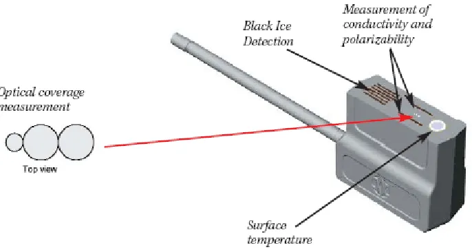
[image:23.595.206.408.333.512.2]The measurement of water layer thickness and the detection of snow or ice on the road surface have been improved by integrating an optical sensor into the road sensor. The optical sensor consists of a construction of optical fibres. The middle fibre emits invisible infra red from the sensor upwards while the two other fibres measure the amount of reflected light. Based on this the sensor is able to measure water layer thickness and the presence of snow and ice.
Fig 3.6 The principle of the optical “eye”
The Finnish Road Administration tested this sensor and in 86% of cases the road state measured was the same as the observed road state. These measurements and others (surface and ground temperature, surface capacitance (for black ice detection) and surface conductivity (for precipitation detection)) are analysed in the ROSA station.
The IceCast system hub provides a robust multi-tasking environment. It manages the collection and handling of observational weather station data.
prediction model. This heat-balance model takes as input forecasts of air and dew point temperature, wind speed, cloud amount and type and rainfall measurements. This data is collected at 3 hourly intervals over a 24 hour period. When the model is run, the output consists of road surface temperatures at hourly intervals and a forecast of the road surface state. Local authority engineers connect to Met Éireann’s server and view the latest forecasts.
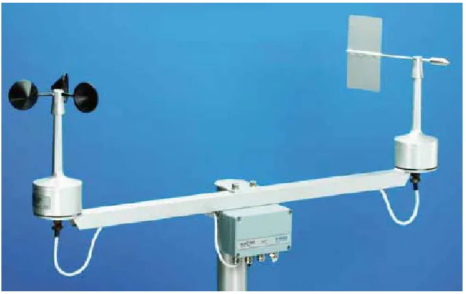
[image:24.595.132.472.339.554.2]The anemometer (WAA151) likely in use by the NRA has an operating range of 75 m/s or 167.8 mph. A wind-rotated chopper disc attached to the shaft of the cup wheel cuts an infrared light beam 14 times per revolution and this generates a pulse from the phototransistor. This pulse rate is directly proportional to the wind speed. There is a heating element in the shaft tunnel to prevent the bearings from freezing.
Fig 3.7 WA15, complete with anemometer and wind vane
The wind vane (WAV151) is counter-balanced, low-threshold and optoelectronic. Infrared LEDs and phototransistors are mounted on six orbits on each side of disk. When the vane turns, the disk creates changes in the code received by the
phototransistors. The code is changed in steps of 5.6°. There is also a heating element in the wind vane.
• Wind tunnel tests
• Vibration tests
• Humidity tests
• Salt fog tests
3.4. Review of Open Source GIS Systems
Geographic Information Systems (GIS) are a combination of spatial data, hardware, and software that allow for complex analysis and querying of mapped information. The successfulness of this research undertaking is heavily dependent on the choice of GIS. The following criteria were used to shortlist candidates:
• Component model
• Relevant APIs
• Data format support
• Usage community
• Robustness
• Lifetime
Sources of information were:
• http://www.freegis.org
• http://www.opensourcegis.org
3.4.1. GRASS (Geographic Resource Analysis
Support System)
(http://grass.itc.it)
GRASS is certainly the largest GIS open source software project. It is written in C and operates through a graphical user interface and shell in X-Windows. A 464 page book is available. GRASS has portability problems on windows (experimental at the
Component model
The GRASS GIS needs to be installed on a server to get the system running. The GRASS GIS is a fully fledged backend processing system, so it would have the capability to implement online systems with spatial analytical capabilities rather than providing visualizations on the clients, which is commonly available in other Web GIS applications. Attributes can be stored in many ways in (external) databases. All
attributes are handled through a common layer called the DBMI library (DataBase Management Interface) which provides several drivers including ODBC.
Relevant APIs
For programming a fully documented C-API (> 800 GIS functions) is provided. Java interfaces are also offered. GRASS-JNI allows programmers to access GRASS data from applications written in Java. It uses JNI (Java Native Interface) language to use the GRASS library and its API closely resembles the GRASS Programmers' API.
Data format support
GRASS can import/export lots of image, raster and vector formats, however there is currently a bug reported against the import of MIF/MID files (MapInfo).
Usage community
GRASS has involved a large number of federal US agencies, universities, and private companies. GRASS is currently used in academic and commercial settings around the world, as well as many governmental agencies including NASA, The National Park Service and The US Census Bureau.
Robustness
Users can write their own code to interface with the documented GIS libraries and by using the GRASS Programmers Manual.
Lifetime
released 1985 and GRASS 5.3 was released in May 2004. GRASS 5.7 is currently under development.
3.4.2. JUMP (Java Unified Mapping Platform)
(http://www.vividsolutions.com/jump)
JUMP is written in 100% pure Java and is a GUI-based application for viewing and processing spatial data.
Component model
JUMP’s workbench for viewing and processing data loads extensions (jar files) on start up such as renderers, plug-ins, curser tools and data sources that uses JUMP’s data structures to draw, load, save and manipulate drawings.
Relevant APIs
JUMP provides APIs exposing all core classes. JUMP provides an API giving full programmatic access to all functions, including I/O, feature-based datasets,
visualization, and all spatial operations. Documentation is available for these API’s.
Data format support
The JUMP geometry model supports all open GIS Consortium data types.
Usage community
Two user communities exist for JUMP. The workbench can be used by anyone who wants to view or process spatial data. Access is given to all APIs that JUMP uses, so developers use the APIs for developing their own applications.
Robustness
be displayed. The JUMP Workbench is designed to be highly modular, open and extensible. New functionality can easily be added and has access to all Workbench components and functions.
Lifetime
JUMP 1.0 was released only in June 2003 and 1.1 in November 2003.
3.4.3. MapServer
(http://mapserver.gis.umn.edu)
MapServer is not a full-featured GIS system but allows users to create "geographic image maps", that is, maps that can direct users to content. MapServer focuses on web mapping and not GIS services. MapServer can display high-quality thematic maps, but it apparently lacks analytic functions of any kind. A GPS tracking system is available as a demo.
Component model
The software builds upon other popular OpenSource or freeware systems like Shapelib, FreeType, Proj.4, GDAL/OGR and others.
Relevant APIs
The MapServer system now supports MapScript which allows popular scripting languages such as Perl, Python, Tk/Tcl, and Java to access the MapServer C API.
Data format support
Vector and raster formats supported.
Usage community
Robustness
MapServer will run on Linux/Apache platforms and is known to compile on most versions of Linux/UNIX, MS Windows and MacOS.
Lifetime
MapServer was originally developed by the University of Minnesota in cooperation
with NASA and the Minnesota Department of Natural Resources.MapServer 1.0 is
around since 1997 and is currently at 4.02.
3.4.4. GeoTools
(http://www.geotools.org)
It is written in Java and is designed to be used by developers for developing geospatial services and applications. It is the leading GIS open source Java library.
Component model
GeoTools is a Java toolkit for developing interactive geographical maps. GeoTools puts emphasis on the client side mapping applets which require little or no server support. The components that make up the GeoTools architecture are Viewer, Scaler, Theme, Layer, Shader, GeoData, Highlight Manager and Shade Style.
Relevant APIs
GeoTools provides over 110 packages with over 1300 Java classes.
Data format support
It supports data source formats such as MapInfo (MIF and MID) and VPF (Vector Product Format). Among the data store formats supported are mySQL (work in progress).
Usage community
Robustness
New map layers can be added easily and all classes come with an abundance of operations. The source code can be recompiled easily.
Lifetime
Work began in 1996 at the University of Leeds. GeoTools is not yet finished but offers many features, the last release was GeoTools 2.0-B4 in May 2004. It has about 117,500 downloads to its credit (sourceforge.net).
3.4.5. OpenMap
(http://openmap.bbn.com)
Component model
OpenMap is a Java Beans based toolkit for building applications and applets needing geographic information. OpenMap provides a set of Swing components that understand geographic coordinates. These components help display map data, and help handle user input events to manipulate that data.
Relevant APIs
OpenMap is primarily for data viewing and offers very little in the way of analysis functionality.
Data format support
The MapInfo functionality in OpenMap supports MIF files, however does not support MID or TAB files. However, TAB files can apparently be exported to MIF using MapInfo.
Usage community
worldwide. BBN Technologies finds that OpenMap provides most customers with 90% of the solution they need and BBN provides consulting for the remaining 10%.
Robustness
OpenMapTM is a trademark of BBN Technologies however users are free to add
features/change source code.
Lifetime
A company called BBN Technologies began developing OpenMap as a web-based client-server tool in 1995 and released it as open source in 1998. It is a member of the Open GIS Consortium since 1995. The latest version is OpenMap 4.6, released February 11, 2004.
3.5. Evaluation of Open Source GIS Systems
3.5.1. GRASS
The evaluation of GRASS was first attempted on a windows environment using (Cygwin/X) which is a linux-like environment for windows. Cygwin 1.5.10-3 tools were installed by selecting all available packages. To use the graphical output an XServer and X11 libraries were required, these were apparently available using the XFree86 options in the Cygwin program setup, however these packages seemed to have been removed from this version. To use winGRASS with the X11 display, precompiled Tcl/Tk libraries (version 8.3.4 was installed) were needed. Finally GRASS 5.0.3 was installed. The graphical output failed to work successfully, along with problems with spaces in files names etc. so the linux implementation of GRASS looked increasingly more attractive and stable.
is not a desired requirement for this project; the message passing (in terms of database queries) between client (e.g. web client) and server will be minimal. GRASS provides a tool for converting MapInfo files to GRASS format, however there is a bug logged against this at the moment and has not been fixed yet; nevertheless, it shouldn’t take a long time to develop a parser to fulfil our needs.
3.5.2. JUMP
The JUMP workbench was evaluated is a practical tool for viewing and processing spatial data. This tool could be useful later adding layers to the maps. The developers of this application; Vivid Solutions, have produced a Java Topology Suite (JTS) which is a really useful API of 2D spatial predicates and functions for scenarios like intersection. The technical specifications, javadoc and a developer’s guide are available for the APIs. These APIs will be useful for the journey time estimator project.
3.5.3. MapServer
This application focuses on map generation or maps that can direct users to content. MapServer is installed and run on a Web Server. MapServer’s features are
characterised by the output format of the maps generated. MapServer may be useful later if the client needs a map to be directed to content e.g. average journey time for a road segment.
3.5.4. GeoTools
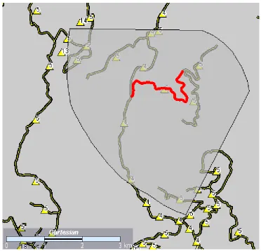
GeoTools was evaluated using sample code and a sample shapefile data set (SpearFish). This GIS application was running as a desktop application. “A shapefile stores
nontopological geometry and attribute information for the spatial features in a data set. The geometry for a feature is stored as a shape comprising a set of vector coordinates” [19]. The Evaluation map had six layers including roads and sites. The shapefile was easily parsed and the features and attributes were extracted. The roads were represented using polylines and the sites represented using polygons. Operations evaluated included
• intersection, which finds the point(s) where two geometries intersect, e.g., a line and a polygon (could be useful for roads and weather station sites).
• distance, which finds the closest distance between two geometries, e.g., a point and a line (could be useful for mapping vehicle position to road segments).
Lots of other operations evaluated also such as: getLength, getArea. See below for a graphical demo of road segments, areas (polygons, e.g., meterlogical area or road event impact) and one highlighted segment, perhaps road closure.
The MathTransform interface is used to apply transformations in GeoTools.
A factory class exists to create a CoordinateTransformation from source and target
CoordinateSystem objects. Pre-made static objects exist in GeoTools such as WGS84 (an earth-fixed Cartesian coordinate system) make it easy to reference commonly used
coordinate systems. CoordinateSystem objects can also be made by hand by parameter
setting (e.g. true and false origins, semi major and semi minor axes) or from well known text embedded in strings parameters.
A MathTransformFactory can also be used in GeoTools, which is a lower level API to give the user more control when creating transforms. Among the key words available to
create a transform is Transverse_Mercator.
Creating a projected coordinate system (in the case of this project, to the National Irish Grid) should not be a difficult task using GeoTools.
3.5.5. OpenMap
Fig 3.8 Sample Data Set evaluated using GeoTools
3.5.6. GIS Evaluation Conclusion
GeoTools was used in this project because:
# Fully Featured GIS
# Has Coordinate Transformation Libraries
# Vast amount of APIs (≈110 packages, ≈1300 classes)
# Ongoing development since 1996
# Multiple file format support
# Robust
# Source code can be recompiled easily
4. DESIGN
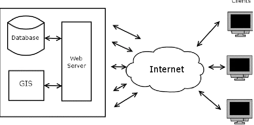
[image:35.595.91.515.166.375.2]This chapter details design decisions made to implement a Journey Time Estimation System. Fig 4.1 shows a high-level view of how the final product may be deployed.
Fig 4.1 Deployment Diagram
The process running on the web server will access only two components; the database where the journey times and context data is stored and the Geographic Information System so that the server process can check which journey times need to be tagged with which context data.
The following sections in this chapter outlines the key modules in the journey time estimator.
4.1. GPS Data Acquisition
The GPS data is available in batches and is batch processed. The GPS data is in csv (comma separated value) format. There are a number of ways to read the batch data.
2. ‘Load’ the batch data into the database and leave the database decide the columns.
3. Treat the batch data as an ODBC (Open Database Connectivity) data source.
Option 1 could be considered as overkill given that each line of the data is a GPS reading and the values are separated by commas, i.e. the data source already has a structure. Option 2 would load the contents of the entire batch of data into the database which isn’t required. Option 3 is a robust solution. As an ODBC data source, the querying component has the flexibility of using SQL to retrieve values in a speedy fashion.
Fig 4.4 shows the data schema for the journey times. One of these records exists for each one-way journey undertaken by a vehicle between two adjacent towns i.e. one road segment. The start time and finish time are necessary (as oppose to just the journey duration) so that this data set can be tagged later with contexts that have the same or similar extent in time. A schema exists for storing a town also as shown in Fig 4.2.
Fig 4.2 Town Schema
Fig 4.3 Road segment schema
| Fi el d | Type | Nul l | Key | Defaul t | Extr a
-- - -- - -- - -- -- - -- - -- - -- - -- - -- - -- - -- -- - -- - -- - -- - -- - -- - -- - -- -- - - -- - -- - -- - -- -- - -- - -- - -- - -- - -- - -- - - | i d | i nt ( 10) unsi gned | | PRI | NULL | aut o_i ncr ement | s egment _i d | i nt ( 11) | YES | | NULL | | s tar t _t i me | char ( 25) | YES | | NULL | | fi ni s h_t i me | char ( 25) | YES | | NULL | | Fi el d | Type | Nul l | Key | Defaul t | Extr a -- - -- - -- - -- -- - -- - -- - -- - -- - -- - -- - -- -- - -- - -- - -- - -- - -- - -- - -- -- - - -- - -- - -- - -- -- - --
| i d | i nt ( 10) unsi gned | | PRI | NULL | aut o_i ncr ement | or i gi n | i nt ( 11) | YES | | NULL |
| dest i nat i on | i nt ( 11) | YES | | NULL | | dis t ance | doubl e | YES | | NULL | | r oad_number | char ( 5) | YES | | NULL |
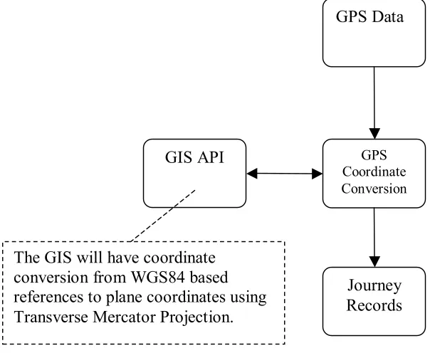
4.2. GPS Coordinate Conversion
[image:37.595.115.417.214.462.2]Conversion must be done from the GPS Geodetic Coordinates (based on WGS84 references) to the Irish National Grid plane coordinates. An implementation of this has already been written in C and MapBasic (former project, see section 1.2) however an implementation using Java and GeoTools would be desirable.
Fig 4.5 Coordinate Conversion
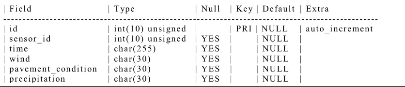
4.3. Context Acquisition
Context data from the sensors in the environment needs to be collected and stored in a database. At the moment this information is available in batches of ASCII files. These files will need to be parsed to extract the appropriate values and then new records will need to be generated from this data. The same decision process was used as in section 4.1 above for reading the context data. These new records should then be uploaded to a data base so that the data can be correlated with the journey times. Fig 4.6 below show the weather data schema, one of these records will represent the data retrieved from each periodic poll of the weather stations.
GPS Data
GPS Coordinate Conversion
GIS API
Journey Records The GIS will have coordinate
Fig 4.6 Weather data schema
Fig 4.7 Context Acquisition
Note that there is no interaction with the GIS here. This will not be done until the user queries the system to retrieve contextualised journey times.
4.4. Context Application
Journey records are essentially the start and finish time of vehicles on the road
[image:38.595.154.457.219.397.2]segments. This data needs to be tagged with context data to produce route profiles for the road segments. One way to correlate journey records and context information is via a relational database. The context data also needs to know properties about the sensors in order to do the map matching. Properties would include the grid coordinates of the sensor.
| Fi el d | Type | Nul l | Key | Defaul t | Extr a
-- - -- - -- - -- -- - -- - -- - -- - -- - -- - -- - -- -- - -- - -- - -- - -- - -- - -- - -- -- - - -- - -- - -- - -- -- - -- - -- - -- - -- - -- - -- - -- -- | i d | i nt ( 10) unsi gned | | PRI | NULL | aut o_i ncr ement | s ens or _i d | i nt ( 10) unsi gned | YES | | NULL |
Fig 4.8 Sensor Data Schema
Fig 4.9 Context Application
The context could also be represented in a hierarchy. Some research articles call these levels: mission, major and sub-contexts or contexts, features and values.
Fig 4.10 A hierarchical way to represent context
In this project the context will be stored in database records without the hierarchical data structure.
| Fi el d | Type | Nul l | Key | Defaul t | Extr a
-- - -- - -- - -- -- - -- - -- - -- - -- - -- - -- - -- -- - -- - -- - -- - -- - -- - -- - -- -- - - -- - -- - -- - -- -- - -- - -- - -- - -- - -- - - | i d | i nt ( 10) unsi gned | | PRI | NULL | aut o_i ncr ement | name | char ( 30) | YES | | NULL | | east i ng | doubl e | YES | | NULL | | nor t hi ng | doubl e | YES | | NULL | | r ange | doubl e | YES | | NULL | | extent | doubl e | YES | | NULL |
Weather
Wind Precipitation Pavement Condition
Dry Icy
Wet High Wind
No Wind No Rain
Rain
Snow
Journey Records
Context Data
GIS Records Journey
4.5. Traveller Information System
[image:40.595.114.543.207.530.2]The traveller information system will be in the form of web server. The web server collects all the required journey times from the journey time database and correlates this information with the context data. This is depicted in Fig 4.11 below.
5. IMPLEMENTATION
5.1. Pre-Processing of Map Data
The digital representation of the Irish national primary route network was received from the National Roads Authority of Ireland (NRA). This representation was compiled using vehicles (with GPS receivers) travelling the route network. The file format of the roads representation was in a MapInfo® format. At the time of implementation,
GeoTools does not support MapInfo® format. A popular format that geotools does support is ERSI shapefiles. MapInfo Professional was used to convert the MapInfo files to shapefile format.
After converting the files to shapefiles a problem was encountered whereby the
segments of roads did not correspond to inter-urban line segments. Fig 5.2 depicts why the pre-processing was necessary, some segments traversed over towns (E.g. 6, 7 of left map), while others represented half of an inter-urban road segment (E.g. 3, 8 of left map). This is a problem because the inter-urban line segments need to be represented as objects in the running software so that operations can be performed such as distance and start and end point of inter-urban line segments. The map data needs to be pre-processed before it can be used in a GIS application.
Fig 5.2 Motivation for Pre-Processing
Algorithm:
1. Read all features from the road shapefile. (features read using
org.geotools.data.FeatureReader)
2. Get all road numbers (e.g. N1..N86) from 1. (getRoadNumbers(), the road
number is an attribute and was read using getAttribute("ROAD") from the
FeatureReader package)
3. Generate routes (e.g. 86 routes) using 1 and 2 above. (getRoads(), select all
roads from the road set ordered by road number and union the roads
(geometries) with a similar road number together.
4. Read all features from the town shapefile. (getTowns(), get a list of all towns
in the shapefile, towns are read using getAttribute("TOWNNAME"))
5. Generate inter-urban new road segments using 3 and 4 above.
(getRoadSegments())
6. Write new inter-urban road segments to a new shapefile using 5 above.
(writeToFile(), writes the new geometries to the new shapefile and the new attributes (road name, origin, destination) to the associated dbf file. This is
accomplished using org.geotools.data.shapefile.shp.ShapefileWriter package
5.2. Coordinate Conversion
5.2.1. Introduction
The journey time estimator system is based on the use of Global Positioning System (GPS) data provided by a fleet of probe vehicles. This data needs to be matched with a map of routes in order to create route profiles. The digital map of routes and towns of Ireland available for this project are referenced using the Irish Grid reference system.
5.2.2. The Irish Grid Reference System
The Irish Grid is a plane co-ordinate system based on a modified Transverse Mercator
Projection. The Irish Grid was developed over more than two hundred years, beginning in 1783 with the Principal Triangulation, which finished in 1832. The Ordnance Survey of Ireland (OSi) carried out a Primary Triangulation (or re-triangulation) of Ireland from 1958 to 1969. In 1975, one adjustment was made (called the 1975 Mapping Adjustment) to produce latitude and longitude positions (geographic co-ordinates) for the primary stations in the reference frame. A modified Airy ellipsoid was used as a model for the earth.
The OSi projects geographic co-ordinates onto the Irish Grid using standard Transverse Mercator projection with Irish parameters (Fig 4). Positions on an Irish Grid are
expressed in two dimensions as Easting (E) and Northing (N) relative to a false origin.
5.2.3. The Modified Airy Ellipsoid
Fig 5.3 Airy Modified is a better fitting for Ireland rather than GRS80
5.2.4. The
Transverse
Mercator
Projecting coordinates from a curved surface onto a flat surface will cause some distortion, but given an appropriate projection system for a region the distortion can be minimised. One projection which retains shape and scale is the Transverse Mercator Projection.
[image:44.595.128.479.472.705.2]A cylinder is wrapped around the ellipsoid so that its circumference (or some of it) touches the ellipsoid along a line of longitude i.e. the central meridian. The radius of the cylinder will match the ‘radius’ of the ellipsoid at one point only, this is the true origin. The origin is chosen to be a central area of the area being projected e.g. the middle of Ireland. The cylinder is then unwrapped providing a flat surface.
The scale of the projected area is correct along the central meridian. However the scale away from the central meridian increases in a uniform way and this can be corrected by applying a scale factor. The scale factor is dependent on the position of the region on the globe.
For convenience purposes a false origin is introduced to rid the coordinate points of negative values. Two constants, one for east coordinates and one for the west coordinates are added to coordinates referenced from the true origin.
5.2.5. Coordinate
Conversion
Fig 5.5 Goal of the Coordinate Conversion Module
Ellipsoid Semi-Major Axis (Airy Modified) 6377340.189 m
Semi-Minor Axis (Airy Modified) 6356034.447 m
True Origin Latitude 53.5 º N
Longitude (Central Meridian) 8.0 º W
False Origin False Easting 200000 m
False Northing 250000 m
Scale Factor 1.000035
Two methods of coordinate conversion in GeoTools were evaluated:
Method 1. Modify Transverse Mercator Projection
A Transverse Mercator Projection implementation is available in the GeoTools2 coordinate transformation package. Relevant parameters can be set to achieve a modified projection. The above Irish parameters (Fig 5.6) were used to create a modified Transverse Mercator Projection.
Method 2. Use CoordinateTransformationFactory
CoordinateTransformationFactory can be used to automatically create transformations
given two CoordinateSystem objects. CoordinateSystem objects can be created by using
pre-made static objects or writing a definition. One such pre-made static object is WGS84 which defines the source coordinate system. No such static object exists for the Irish Grid, so one was created using WKT (Well Known Text) strings to define the coordinate system. The Irish parameters above were used to define the coordinate system.
5.2.6. Evaluation
of
Coordinate Conversion
Two sample computations of coordinate conversion were given in [21].
Location Latitude (Φ) Longitude (λ) Easting (E) Northing (N)
OSO1 53º 21’ 50.5441” 06º 20’ 52.9181” 309958.2645 236141.9291
Howth 53º 22’ 23.1566” 06º 04’ 06.0065” 328546.3442 237617.1863
Fig 5.7 OSi Computations of E and N from Φ and λ
Method 1 Method 2
Location Easting (E) Northing (N) Easting (E) Northing (N)
OSO1 309958.26446095 236141.92909108 309972.85087006 236140.22002974
Howth 328546.34421915 237617.18633968 328563.39666628 237615.66433080
Fig 5.8 GeoTools Computations of E and N from Φ and λ
Using the GeoTools Transverse Mercator implementation and applying the irish parameters (Method 1) appears to work perfectly.
5.2.7. A New Coordinate System
In recent times, the deployment of new technologies, such as GPS and more
computationally powerful computers has highlighted some shortcomings of reference systems. With the advent of GPS it is now more appropriate to maintain accuracy of the survey by using a coordinate system that is compatible with GPS so that there would be little distortion. This is the case for a new projection system for Ireland not using the modified Airy Ellipsoid (a regional ellipsoid) but an accepted global one such as GRS80.
This is a new projection called the Irish Transverse Mercator Projection.
The coordinate conversion can be easily switched to project onto the Irish Transverse Mercator by substituting the parameters above in Fig 4 with new parameters that can be found in [22]. Of course a digital map with points referenced using the Irish Mercator Projection is also required.
5.3. GPS Data Processing
96253817,2003-04-03 16:03:00,"-6.374623055555555","53.485321666666664",71,"30040310030b7a0956fea1d4dc00c641",1491,,5,,,1,"1",,2003-04-05 06:29:47.100000000, 96253818,2003-04-03 16:03:00,"-6.373231388888889","53.48373333333333",68,"30040310030b79f300fea1e86e00bd41",1491,,5,,,1,"1",,2003-04-05 06:29:47.117000000, 96253819,2003-04-03 16:03:00,"-6.370569722222222","53.48078833333334",74,"30040310030b79c996fea20ddc00ce41",1491,,5,,,1,"1",,2003-04-05 06:29:47.133000000, 96253820,2003-04-03 16:03:00,"-6.369043055555555","53.47911833333333",79,"30040310030b79b21afea2235400dc41",1491,,5,,,1,"1",,2003-04-05 06:29:47.133000000, 96253821,2003-04-03 16:04:00,"-6.365974722222222","53.47575666666667",72,"30040310040b7982d4fea24e7a00ca43",1491,,5,,,3,"1",,2003-04-05 06:29:47.150000000, 96253822,2003-04-03 16:04:00,"-6.364483055555556","53.47413",72,"30040310040b796bf4fea2637400c841",1491,,5,,,1,"1",,2003-04-05 06:29:47.163000000, 96253823,2003-04-03 16:04:00,"-6.361536388888889","53.47091833333333",72,"30040310040b793ecafea28ce400c842",1491,,5,,,2,"1",,2003-04-05 06:29:47.163000000, 96253824,2003-04-03 16:04:00,"-6.360128055555555","53.46933666666666",70,"30040310040b79288cfea2a0b200c441",1491,,5,,,1,"1",,2003-04-05 06:29:47.180000000, 96253825,2003-04-03 16:05:00,"-6.357316388888889","53.46618333333333",74,"30040310050b78fc34fea2c83c00cf41",1491,,5,,,1,"1",,2003-04-05 06:29:47.193000000, 96253826,2003-04-03 16:05:00,"-6.355789722222222","53.464535",77,"30040310050b78e506fea2ddb400d743",1491,,5,,,3,"1",,2003-04-05 06:29:47.210000000, 96253827,2003-04-03 16:05:00,"-6.3529430555555555","53.461345",66,"30040310050b78b82afea305bc00ba41",1491,,5,,,1,"1",,2003-04-05 06:29:47.210000000, 96253828,2003-04-03 16:05:00,"-6.351594722222222","53.45986",66,"30040310050b78a348fea318b200b841",1491,,5,,,1,"1",,2003-04-05 06:29:47.227000000, 96253829,2003-04-03 16:06:00,"-6.349169722222222","53.45705",59,"30040310060b787bc4fea33acc00a642",1491,,5,,,2,"1",,2003-04-05 06:29:47.240000000,
Fig 5.9 Sample GPS Data
Fig 5.10 GPS Processing Class Diagram
id (integer unsigned, key) name (char(30)) 1 Slane 2 Ashbourne 3 Ardee 4 Kells 5 Castleblaney 6 Navan
[image:48.595.155.448.597.735.2]id
(integer unsigned, key)
origin (integer) destination (integer) distance (double) road_number (char(5))
1 1 2 22140.09 N02
2 7 5 13602.75 N02
3 3 7 16081.73 N02
4 4 6 13072.78 N03
5 8 9 5027.15 N06
Fig 5.12 segments Table with Sample Data
id
(integer unsigned, key) segment_id (integer) (char(25)) start_time finish_time (char25))
1 4 2003-04-01 14:40:00 2003-04-01 14:50:00
2 3 2003-04-02 13:42:00 2003-04-02 13:55:00
3 2 2003-04-02 13:59:00 2003-04-02 14:10:00
4 1 2003-04-03 14:32:00 2003-04-03 14:47:00
[image:49.595.84.522.100.193.2]5 5 2003-04-04 17:16:00 2003-04-04 17:20:00
Fig 5.13 journey_times Table with Sample Data
The GPS readings are processed one by one using the algorithm below. In order for a journey to be classified as valid then the following must be true:
• A vehicle must travel along a national primary route between adjacent towns. If
a vehicle turns off a national primary route then the position of the vehicle will fail to map onto the road segment and that journey will be void.
• A vehicle must maintain sufficient progress along a road segment. If a vehicle
stops or slows down, then subsequent GPS reading will prove that sufficient progress has not been made (progress determined by distance covered in a period of time) to classify this journey as valid.
• A vehicle must first enter the bounds of the originating town, leave the bounds
of the originating town and enter the bounds of the destination town. Of course the destination town will then become the originating town if the vehicle proceeds onto another road segment.
When the GPS processing is started a MapOfRoadSegments is created. This object
region is created to allow for inaccuracy of the GPS readings. See Map Matching, section 5.4.
Journey Identification Algorithm:
While (get next record ≠ eof) Begin
Convert longitude and latitude If position is in a town
Begin
If start_town == null OR start_town == current position Begin
start_town = current position start_time = current time End
Else Begin
If sufficient progress was made Begin
finish_town = current position
finish_time = current time
Write journey (start_town, finish_town, start_time, finish time) start_town = finish_town
start_time = finish_time End
End End
Else If position lies on a road AND start_town ≠ null If sufficient progress was not made
start_town = null
Else If position does not lie on a road
start_town = null
Fig 5.14 Journey Identification Algorithm
5.4. Map-Matching
There are three classifications of GPS data in this project: 1. Vehicle lies within a town boundary.
public String inTown(double x, double y)
This function returns the town name if the point lies within a town otherwise null. This checking is accomplished using the contains method in the
com.vividsolutions.jts.geom.Geometry package.
2. Vehicle lies along a road segment.
public static boolean inRoadBuffer(double x, double y)
This function returns true if the point lies within a road buffer otherwise false. In this Project the road buffer was set as 200 meters (i.e. 200 meters either side of the road)
(Road buffer was created using
com.vividsolutions.jts.operation.buffer.BufferBuilder)
Fig 5.15 Road Buffers Illustration
5.5. Context Data Processing
The context data for this project contains the name or id of the sensor where the data was acquired from. In order to tag the journeys with context data, the location of the sensors is essential for checking if the road segments and context data are in the same vicinity.
The Sensor information is recorded in a flat ASCII file and is read when the Context data processing takes place. The range of a sensor is the area around the sensor that the data is deemed valid. For example if the range of a sensor is 30 km, then any road segments that lie within this range around that sensor is tagged with data from that sensor if the times correspond. The extent of a sensor is the length of time that data is valid given the context data. For example, weather information is collected every sixty minutes from the weather stations so the extent of the weather sensor is sixty minutes.
name,easting,northing,range,extent
M7 Portlaoise Bypass,248400,196500,30,30 N10 Kilkenny,250100,152300,30,30
N81 Baltinglass,290900,197400,30,30 N11 Arklow Bypass,325900,176900,30,30
Fig 5.17 Weather Processing Class Diagram
5.6. Web Interface
The Traveller Information System running on a web server consists of a Servlet
accessing the journey time records, context data records and the GIS application. Upon receiving a post request from one of the client the server get three parameters:
• Origin
• Destination
• Time of Day (time periods in Fig 5.18)
Time of Day Start time Finish Time
Peak Am 07:00:00 09:59:59
Day 10:00:00 16:29:59
Peak Pm 16:30:00 18:59:59
Night 19:00:00 06:59:59 (next day)
Fig 5.18 Servlet's definition of time periods
The servlet performs the following process:
i. Get all journey records for the submitted origin, destination and time of the day.
[image:53.595.112.488.596.664.2]iv. Display journeys and available contexts.
6. EVALUATION
6.1. Evaluation of GPS Data
[image:55.595.91.538.268.738.2]The correctness of the GPS data was validated by matching the positions recorded with the route network. The trajectory of the vehicle was aligned along the route network without a problem and journey records were obtained. Fig 6.1 below show the journey times obtained from one batch of GPS data. The blank origin or destination corresponds to town in the GIS that was not given a name. The distance given is in meters.
| origin | destination | start_time | finish_time | distance | road_number
The above data set corresponds to the journey times for one probe vehicle fitted with a GPS sensor and can not be a reflection of the journey times for these routes on average. The distances where checked using a road map and were very accurate, given the towns boundaries. A significant amount of vehicles would be required in order to produce more accurate journey times. These journey times would need to be evaluated with surveys or some other means of collecting journey time data, e.g., using a fixed sensors such as inductive loops or infra-red sensors as described earlier in the State of the Art (Chapter 2). This type of infrastructure is unavailable to us.
6.2. Evaluation of Weather Data
The weather data acquired from the road side weather stations was real weather data which was obtained from the National Roads Authority. In order to evaluate the journey time estimation system completely, lots of historical weather data would be required that corresponds with the times in the GPS readings. This data is unavailable to us at the moment and the existence of the data is also questionable. The road side weather data is freely available to the public on an hourly basis, so an archive could be built over time and the archived weather data could be correlated with real GPS data over the same time period.
Fig 6.2 Aggregated weather data from a roadside weather station
6.3. Evaluation of Route Profiles
The Servlet running on a web server correlates the GPS data and the weather data, see section 5.6. The evaluation of the route profiles was performed using the web interface. Given criteria from the client, the servlet retrieved the requested journey times, checked if the road segment lies within a context, found context data for this road segment (if available) and generated route profiles, see Fig 8.2.
| name | time | wind | pavement_condition | precipitation
7. CONCLUSIONS
7.1. Goals Achieved
This project achieved lots of results throughout the course of the project:
• A tool was developed that could be used to provide road management
authorities an indication of the level of service being provided on a road network.
• The tool generates profiles (a route profiling application) of road segments given context information available for the road segments; current traveller information systems only exploit spatial and temporal information.
• The contextualised journey times could be used to identify roads that perform
poorly in adverse weather conditions.
• The contextualised journey times could be used to provide an indication of road
usage patterns, e.g. during heavy precipitation, more people take the car in the morning on a particular route.
• Geotools proved to be perfectly adequate for developing traveller information
systems with respect to journey time estimation.
• Geotools has excellent support for coordinate conversion from longitude and
latitude to the National Irish Grid.
• Geotools is suitable for developing journey time estimators using a set of probe
vehicles tracked by GPS.
• Geotools has support for overlaying context areas on a route network.
• ERSI shapefiles are suitable for representing a road network and context areas.
• Lots of tools are available for viewing and editing ERSI shapefiles.