Abstract—We describe a resource oriented modelling method for robotic flowshops and examplify it on a galvanic plant. We compare the process oriented modelling method with the resource oriented method. The resulting simulation tool can be used for the design of scheduling algorithms. Solutions can be found to compromise between the use of resources and productivity of the plant.
Index Terms—Timed petri nets, hoist scheduling, flexible manufacturing
I. PROBLEM STATEMENT
The increasing use of flexible production environments poses high demands on production planners. Besides the necessity to optimize the stationary production over a long period it is more and more important to be able to change quickly and efficiently between different product modes. For plants with automated transport systems we have to find optimum control sequences for the transporter to meet the requirements. Therefore we have developed a simulation model to find control sequences both for stationary and for flexible production environments.
[image:1.595.80.257.587.703.2]The application considered is a line of basins containing chemical, electrolytic or rinsing bathes served by one or more transporters. The plant consists of m machines M1, …, Mm, an input station M0 and an output station Mm+1 sometimes combined at the same place. The input station contains a set of parts J. Each part has to be processed according to its process plan, the list of the operation times oi, i ∈M at the machines and the transport times tij , i, j ∈M between them.
Fig. 1 Layout of the plant
1
Claudia Fiedler and Wolfgang Meyer are with the Institute of Automation, Hamburg University of Technology, 21071 Hamburg, Germany
(e-mail: [email protected]; [email protected])
The operation times oi of part J are kept in intervals
J J i i
l u,
with a lower bound J i
l and an upper bound J i
u . If the upper bound is equal to the lower bound, we speek of a no-wait condition. The upper bound can be infinity, too. There are one or more transporters Tn concurrently or operating with defined areas on the same or on different tracks. The travel times δij can be constant, additive or Euclidean. Additive travel times follow the triangle equality and Euclidean travel times follow the triangle inequality. They are symmetric (δij=δji) and zero from a machine to itself (δii=0). The transport times tij between the operations oi are the sum of travel times δij and a constant needed for loading and unloading the part. The parts in the input station can be of the same type or of different types. Depending on the types of the parts the goal is either to minimize the cycle time vi for parts of the same type or to minimize the the throughput time in case of different part types.
II. STATE OF THE ART OF SCHEDULING
The general problem is known as robotic flowshop scheduling. The part input sequence (for different parts in the input buffer) has to be specified as well as the sequence of robot moves. [1]and [2] are recommended to get a general idea. We adress the Hoist Scheduling Problem as a special case of robotic flowshops. The operation times are given in intervals. The transporters have Euclidean travel times and loaded transporters are not allowed to wait. The NP-completeness is proven by Crama and Klundert [3]. Phillips and Unger [4] solved the monocyclic case with integer programming. Rodozek and Wallace used a hybrid constraint logic programming (CLP) and mixed integer programming (MIP) algorithm [5]. An overview over different kinds of hoist scheduling problems is given in [6]. They extend the Graham notation applied to robotic flowshop scheduling [2][7] to the varying problems of hoist scheduling.
III. PROCESSBASED MODELLING
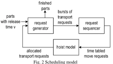
In [8] we presented a process centred modelling method according to the modeling method of [9] for the cyclic hoist scheduling. The general structure is shown in Fig. 2. The parts modelled as process tokens with the processing times as attributes are released to the request generator with constant release time v. The model of the plant (request generator) sends transport requests to the request sequencer if the state of the model has changed because of a finished transport operation and the starting of a tank operation. According to the given priority, the sequencer decides which of the transport request is
Process Centred versus Resource Centred
Modelling for Flexible Production Lines
Fig. 2 Scheduling model
answered next when the transporter is available. Then the time tabled request releases a transporter move if the transporter is not at the needed place. The allocated transporter then causes a transport operation and a new transport request. There are enough process token to lead to a stationary behavior after a transient region at the beginning with the suitable release time V. The start value of V is the sum of the maximal operation time in a tank and the transport times to and from the tank. If a cyclic behavior can not be reached or if the operation times exceed the upper bounds of the given intervals, the release time is increased and the simulation starts again until the given constraints are fulfilled.
[image:2.595.71.269.86.198.2]In the request generator the tank and transport operations of a job are lined up according to the process plan (Fig.3).
Fig. 3 Process plan as A-path
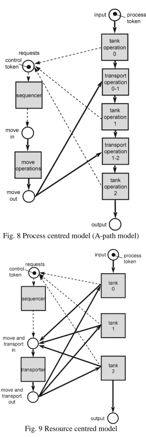
Each operation begins and finishes with a start/stop-transition. This is the so-called A-path. Then the B-path is added: the needed resources for the operations connnected with the start transition of the correspondent operation. In our example we need tank 1 and tank 2 for the tank operations and the transporter for the transport operations. This may vary if there are more transporters or loops in the process plan if a tank is used more than once for a job. Process token symbolize the parts and resource token for the availability of resources are added. A tank resource is occupied if a transport operation to the tank has started and as long the transport operation from the resource has not been finished (Fig.4). The requests are collected in the input place for the sequencer. It is
Fig. 4 A-path and B-path
Fig. 5 Request generator
[image:2.595.125.210.388.572.2]not only important if the transporter is available but also if it is at the needed place. Therefore the transporter availability place is extended to places for the availability at the needed tank (Fig. 5).
[image:2.595.308.540.550.727.2]Fig. 7 Gannt Chart for solution of PhU-benchmark – transporter sequence
Because the loaded transport operations are included in the request generator the transporter model just contains the unloaded movements from each to each other place. Applied to the first benchmark described by Phillips and Unger (PhU) [4] the modelling leads to the optimal solution of 521 seconds for the cycle time V [8]. Fig. 6 shows the gannt chart of the minimal solution of the Phillips/ Unger benchmark problem. The processes are released to the plant with a release time V of 521 seconds and the operation times are given as the lower bounds of the intervals. The rows between two resources symbolise the extension of the operation time from the lower bound. If there is more than one part in the plant the sequencer descides according to the implemented rule the order of loaded and unloaded transport operations for the transporter T as the bottleneck resource.
The descision time of the sequencer is time shifted by the maximal value of the movement time for unloaded transports to enable the transporter to be at the needed tank in due time. The implemented rule here is a special priority rule depending on the size of the operation intervals as described in [8]. The Operation-Due-Date-rule (ODD) wich chooses the next tank dependent on the time difference to the upper bound of the interval leads to good results, too. The more parts are in the plant the more the operation times are extended. After the transient region the transporter shows stationary behavior in the minimal time interval of the release time V=521 seconds. Fig. 7 shows the transporter sequence with the length V. The sequence can be transferred into a programmable logic controller (PLC) to realise the processes with the given constraints in the real plant.
The PhU problem is modelled as a flowline. Therefore deadlocks can not take place. If there are loops in the process plans deadlocks can occur and an deadlock avoidance algorithm has to be implemented. Possibilities to inhibit deadlocks are described in [10]. Our approach is described in chapter V.
IV. RESOURCE CENTRED MODELLING
[image:3.595.354.505.139.590.2]In flexible manufacturing environments there is a fast change in product types. To find sequences for lot switching or for new products the process centred model is unsuitable because for each new
Fig. 8 Process centred model (A-path model)
Fig. 9 Resource centred model
flexibility is reflected in Fig. 9 in the number of process flow connections, too. In the process centred model there is just one way for the parts whereas in the resource centred model the processes can be composed in any order. In [11] the compact modeling as a similar concept is described and the effects on the number of petri net elements are determined.
V. DEADLOCK AVOIDANCE
In Discrete Event Systems with loops in the process plans deadlocks may occur. We therefore need a deadlock avoidance algorithm in the resource centred model to enable the model to simulate processes with loops in the plan. The idea is to prevent the last change in the state of the plant which closes a deadlock. The following example may illustrate the algorithm:
Given are three resources a1, a2 and a3. Each resource has capacity one. Then each resource can handle just one of the processes. For process P1 the actual resource may be a1, for process P2 a2 and for P3 a3. Then these four possibilities for the following two resouces for the three processes are possible:
(
)
(
)
(
)
(
)
(
)
(
)
(
)
(
)
(
)
(
)
(
)
(
)
1 2 1 2 1 2 3 1 3
1 3 1 2 3 2 3 2 3
1 2 3 2 1 3 3 1 2
1 3 2 2 3 1 3 2 1
a a a a a a a a a
a a a a a a a a a
P1 P2 and P3
a a a a a a a a a
a a a a a a a a a
; = = = .
Each combination of the three processes P1, P2 and P3 is a deadlock with either size 2 if two processes or resources are involved or size 3 for three involved processes. For example, if P1=(a1 a2 a1) and P2=(a2 a1 a2) then there is a deadlock because P1 blocks the next tank of P2 and P2 uses the next resource of P1. A deadlock with size 3 occurs if P1=(a1 a2 a1), P2=(a2 a3 a2) and P3=(a3 a1 a3) because there are three involved processes and for each of the three processes there exist a process which uses the next resource.
That means there is a deadlock if :
Let P be the set of processes in the plant
{
P1 Pn}
nP= ... ; ∈ℕ (1) and each Pi consists of the actual and the next operation,
(
i i)
i actual next
P= a a ; i =1...n (2) then there exists a subset Q of P
{
1 m}
; = Q...Q ;m
⊆ ∈
Q P Q ℕ (3)
with
=
Q Q
actual next
A A (4) where AQactual is the set of the actual resources occupied by the processes of Q and AQnextthe set of the next resources used by the processes of Q.
In the implementation of the resource centred model then we have to prohibit the transport of the last part to that resource which leads to (4) and results in a deadlock.
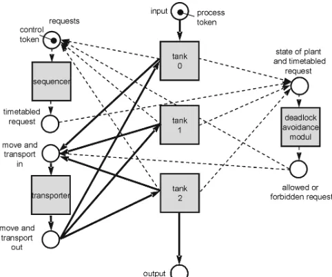
[image:4.595.307.548.276.477.2]In Fig. 10 the simplified model with deadlock avoidance is displayed. The timetabled request is send from the sequencer to the deadlock avoidance modul with information about the actual and the next two resources. The algorithm descides if a deadlock occurs if the process will be transported to the next tank. If so the deadlock avoidance modul sends an inhibit signal to the sequencer for this process and tries the next one. Every time the state of the request generator will change caused by a transport operation all the inhibited requests stored in the deadlock avoidance modul are tested whether the danger for deadlock still holds or not. The sequence decision for concurrent processes is based on the due date of the tank operation the transport would finish. Other priority decisions are possible, too.
Fig. 10 Resource centred model with deadlock avoidance module
VI. ILLUSTRATIVE EXAMPLE
The implemented simulation tool can be used for scheduling algorithms decisions. The result is a transporter sequence in a textfile which can be directly transfered into a PLC to control the transporter. The input is an Excel file with the process plan and the transporter road map. The model is implemented in PACE 5.0, a simulation tool for coloured timed petri nets. [12] Assume the process plan as given in table 1. There are seven tanks.
The result for the flowline is given in Fig. 11. The minimal stationary solution is V=489.
Fig. 11 Gannt chart for the example in table 1
The operation in tank 1 seems to be the bottleneck. If we add another resource M1 in the line the result can be reduced by 41% to V=292 (Fig. 12). Now the transporter is fully occupied and it is unlikely to find a smaller solution without adding another transporter.
Fig. 12 Gannt chart for the example in table 1 with an additional tank 1
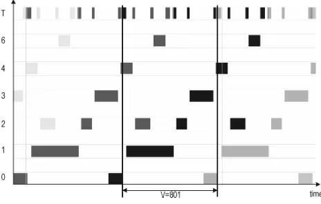
[image:5.595.308.540.191.339.2]If the operation in tank 2 is a rinsing operation and the operation in tank 5 too, we can test what happens if we use just one tank for this operation. Fig. 13 shows the result for just one tank 1 and the loop in the process plan for tank 2. The result of V=801 is really poor. Because of the loop, the smaller stationary solutions found before exceed the upper bounds of the operation times.
Fig. 13 Gannt chart for the example in table 1 with M2=M5
[image:5.595.45.280.288.463.2]But if we add another tank 1 we find a solution of V=385 as the best compromise between the number of resources and the productivity (Fig. 14).
Fig. 14 Gannt chart for the example in table 1 with two M1 and M2=M5
VII. CONCLUSIONS
[image:5.595.48.282.552.724.2]REFERENCES
[1] Y. Crama, V. Kats, J. van de Klundert and E. Levner, “Cyclic scheduling in robotic flowshops” in Annals of Operations Research, vol. 96, pp. 97–124, 2000.
[2] M. Dawande, H.N. Geismar, S.P. Sethi and C. Sriskandarajah,
Sequencing and Scheduling in Robotic Cells: Recent Developments in Journal of Scheduling,.vol. 8, pp. 387–426, 2005.
[3] Y. Crama and J. Klundert, “Robotic flowshop scheduling is strongly NP-complete”, in Ten Years LNMB (W.K.Klein Haneveld, O.J. Vrieze
and L.C.M. Kallenberg, eds.), CWI Tract 122, Amsterdam, pp. 277-286,
1997.
[4] L. W. Phillips and P. S. Unger, “Mathematical Programming Solution of a Hoist Scheduling Program”, AIIE Transactions, vol. 28, no. 2, pp. 219-225, June 1976.
[5] R. Rodošek and M. Wallace, “A Generic Model and Hybrid Algorithm for Hoist Scheduling Problems”, Lecture Notes in Computer Science, vol.1520, pp. 385-399, Springer Verlag, Berlin, 1998.
[6] M.-A. Manier, C. Bloch, “A Classification for Hoist Scheduling Problems”, International Journal of Flexible Manufacturing Systems, vol. 15, no.1, pp. 37 – 55, Jan 2003.
[7] R.L.Graham, E.L. Lawler, J.K. Lenstra, and A.H.G. Rinnoy Kan, “Optimization and approximation in deterministic sequencing and scheduling: A survey”, Annals of Discrete Mathematics, 5, 287-326, 1979.
[8] C. Fiedler, ”Event-driven Generation of Periodic Hoist Schedules”, Proc.
IEEE Conf. Systems, Man, and Cybernetics, Taipei, Oct. 2006.
[9] M. Zhou and F. DiCesare, Petri Net Synthesis for Discrete Event Control of Manufacturing Systems, London: Kluwer Academic Publishers, 1993. [10] M. Lawley, S. Reveliotis, and P. Ferreira, “Design Guidelines for Deadlock-Handling Startegies in Flexible Manufacturing Systems”, The
International Journal of Flexible Manufacturing Systems, Kluwer
Academic Publishers, Boston, 9, pp. 5-30, 1997.
[11] A. v.Drathen, “Compact Modeling of Manufacturing Systems with Petri nets”, Proc. IEEE Conf. Systems, Man, and Cybernetics, Montreal, Oct. 2007.