Many Faces of Feature Importance: Comparing Built in and Post hoc Feature Importance in Text Classification

(1)

Proceedings of the 2019 Conference on Empirical Methods in Natural Language Processing

486

Many Faces of Feature Importance: Comparing Built-in and Post-hoc

Feature Importance in Text Classification

Vivian Lai and Zheng Cai and Chenhao Tan Department of Computer Science

University of Colorado Boulder Boulder, CO

vivian.lai, jon.z.cai, chenhao.tan@colorado.edu

Abstract

Feature importance is commonly used to ex-plain machine predictions. While feature im-portance can be derived from a machine learn-ing model with a variety of methods, the con-sistency of feature importance via different methods remains understudied. In this work, we systematically compare feature importance from built-in mechanisms in a model such as attention values and post-hoc methods that ap-proximate model behavior such as LIME. Us-ing text classification as a testbed, we find that 1) no matter which method we use, impor-tant features from traditional models such as SVM and XGBoost are more similar with each other, than with deep learning models; 2) post-hoc methods tend to generate more similar im-portant features for two models than built-in methods. We further demonstrate how such similarity varies across instances. Notably,

im-portant features donotalways resemble each

other better when two models agree on the pre-dicted label than when they disagree.

1 Introduction

As machine learning models are adopted in so-cietally important tasks such as recidivism pre-diction and loan approval, explaining machine predictions has become increasingly important (Doshi-Velez and Kim,2017;Lipton, 2016). Ex-planations can potentially improve the trustworthi-ness of algorithmic decisions for decision makers, facilitate model developers in debugging, and even allow regulators to identify biased algorithms.

A popular approach to explaining machine pre-dictions is to identify important features for a

particular prediction (Luong et al., 2015;Ribeiro

et al.,2016;Lundberg and Lee,2017). Typically, these explanations assign a value to each feature (usually a word in NLP), and thus enable

visual-izations such as highlighting topkfeatures.

In general, there are two classes of methods: 1) built-in feature importance that is embedded in the machine learning model such as coefficients in lin-ear models and attention values in attention mech-anisms; 2) post-hoc feature importance through credit assignment based on the model such as LIME. It is well recognized that robust

evalua-tion of feature importance is challenging (Jain and

Wallace,2019;Nguyen,2018, inter alia), which is further complicated by different use cases of ex-planations (e.g., for decision makers vs. for de-velopers). Throughout this work, we refer to

ma-chine learning models that learn from data as

mod-elsand methods to obtain local explanations (i.e.,

feature importance in this work) for a prediction

by a model asmethods.

While prior research tends to focus on the inter-nals of models in designing and evaluating meth-ods of explanations, e.g., how well explanations

reflect the original model (Ribeiro et al., 2016),

we view feature importance itself as a subject of study, and aim to provide a systematic character-ization of important features obtained via differ-ent methods for differdiffer-ent models. This view is particularly important when explanations are used to support decision making because they are the only exposure to the model for decision makers. It would be desirable that explanations are con-sistent across different instances. In comparison, debugging represents a distinct use case where de-velopers often know the mechanism of the model beyond explanations. Our view also connects to

studying explanation as a product in cognitive

studies of explanations (Lombrozo,2012), and is

(2)

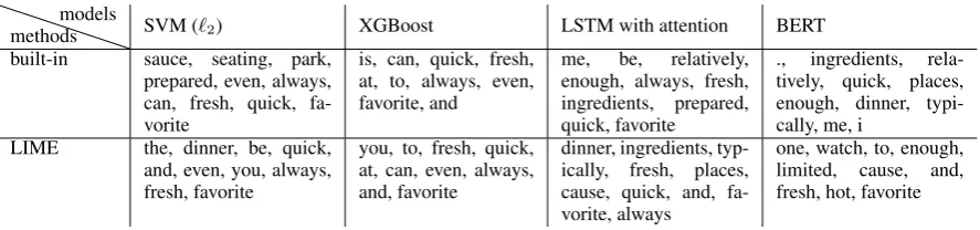
lin-One of favorite places to eat on the King W side, simple and relatively quick. I typically always get the chicken burrito and the small is enough for me for dinner. Ingredients are always fresh and watch out for the hot sauce cause it’s skull scratching hot. Seating is limited so be prepared to take your burrito outside or you can even eat at Metro Hall Park.

methods models

SVM (`2) XGBoost LSTM with attention BERT

built-in sauce, seating, park,

prepared, even, always, can, fresh, quick, fa-vorite

is, can, quick, fresh, at, to, always, even, favorite, and

me, be, relatively,

enough, always, fresh,

ingredients, prepared,

quick, favorite

., ingredients,

rela-tively, quick, places,

enough, dinner, typi-cally, me, i

LIME the, dinner, be, quick,

and, even, you, always, fresh, favorite

you, to, fresh, quick, at, can, even, always, and, favorite

dinner, ingredients,

typ-ically, fresh, places,

cause, quick, and, fa-vorite, always

one, watch, to, enough,

limited, cause, and,

[image:2.595.77.521.100.204.2]

fresh, hot, favorite

Table 1: 10 most important features (separated by comma) identified by different methods for different models for the given review. In the interest of space, we only show built-in and LIME here.

guistic properties important features tend to have. We use text classification as a testbed to answer these questions. We consider built-in importance from both traditional models such as linear SVM and neural models with attention mechanisms, as well as post-hoc importance based on LIME and

SHAP. Table1shows important features for a Yelp

review in sentiment classification. Although most approaches consider “fresh” and “favorite” impor-tant, there exists significant variation.

We use three text classification tasks to charac-terize the overall similarity between important fea-tures. Our analysis reveals the following insights:

• (Comparison between approaches) Deep

learn-ing models generate more different important features from traditional models such as SVM and XGBoost. Post-hoc methods tend to reduce the dissimilarity between models by making im-portant features more similar than the built-in method. Finally, different approaches do not generate more similar important features even if we focus on the most important features (e.g., top one feature).

• (Heterogeneity between instances) Similarity

between important features is not always greater when two models agree on the predicted label, and longer instances are less likely to share im-portant features.

• (Distributional properties) Deep models

gen-erate more diverse important features with higher entropy, which indicates lower consis-tency across instances. Post-hoc methods bring the POS distribution closer to background dis-tributions.

In summary, our work systematically compares important features from different methods for dif-ferent models, and sheds light on how difdif-ferent models/methods induce important features. Our

work takes the first step to understand impor-tant features as a product and helps inform the adoption of feature importance for different

pur-poses. Our code is available athttps://github.com/

BoulderDS/feature-importance.

2 Related Work

To provide further background for our work, we summarize current popular approaches to generat-ing and evaluatgenerat-ing explanations of machine pre-dictions, with an emphasis on feature importance.

Approaches to generating explanations. A bat-tery of approaches have been recently proposed

to explain machine predictions (seeGuidotti et al.

(2019) for an overview), including example-based

approaches that identifies “informative” examples

in the training data (e.g., Kim et al., 2016) and

rule-based approaches that reduce complex

mod-els to simple rules (e.g., Malioutov et al., 2017).

Our work focuses on characterizing properties of feature-based approaches. Feature-based ap-proaches tend to identify important features in an instance and enable visualizations with impor-tant features highlighted. We discuss several di-rectly related post-hoc methods here and introduce

the built-in methods in §3. A popular approach,

LIME, fits a sparse linear model to approximate

model predictions locally (Ribeiro et al., 2016);

Lundberg and Lee(2017) present a unified frame-work based on Shapley values, which can be com-puted with different approximation methods for different models. Gradients are popular for iden-tifying important features in deep learning mod-els since these modmod-els are usually differentiable (Shrikumar et al., 2017), for instance, Li et al.

(2016) uses gradient-based saliency to compare

LSTMs with simple recurrent networks.

(3)

De-spite a myriad of studies on approaches to ex-plaining machine predictions, explanation is a rather overloaded term and evaluating

explana-tions is challenging.Doshi-Velez and Kim(2017)

lays out three levels of evaluations: functionally-grounded evaluations based on proxy automatic tasks, human-grounded evaluations with layper-sons on proxy tasks, and application-grounded based on expert performance in the end task. In

text classification, Nguyen(2018) shows that

au-tomatic evaluation based on word deletion moder-ately correlate with human-grounded evaluations that ask crowdworkers to infer machine predic-tions based on explanapredic-tions. However, explana-tions that help humans infer machine predicexplana-tions may not actually help humans make better deci-sions/predictions. In fact, recent studies find that feature-based explanations alone have limited im-provement on human performance in detecting

de-ceptive reviews and media biases (Lai and Tan,

2019;Horne et al.,2019).

In another recent debate, Jain and Wallace

(2019) examine attention as an explanation

mech-anism based on how well attention values corre-late with gradient-based feature importance and whether they exclusively lead to the predicted la-bel, and conclude that attention is not explanation.

Similarly,Serrano and Smith(2019) show that

at-tention is not a fail-safe indicator for explaining machine predictions based on intermediate

repre-sentation erasure. However, Wiegreffe and

Pin-ter(2019) argue that attention can be explanation

depending on the definition of explanations (e.g., plausibility and faithfulness).

In comparison, we treat feature importance it-self as a subject of study and compare different approaches to obtaining feature importance from a model. Instead of providing a normative judgment with respect to what makes good explanations, our goal is to allow decision makers or model devel-opers to make informed decisions based on prop-erties of important features using different models and methods.

3 Approach

In this section, we first formalize the problem of obtaining feature importance and then introduce the models and methods that we consider in this work. Our main contribution is to compare im-portant features identified for a particular instance through different methods for different models.

Feature importance.For any instancetand a

ma-chine learning modelm:t→y ∈ {0,1}, we use

method h to obtain feature importance on an

in-terpretable representation oft,Itm,h ∈Rd, where

dis the dimension of the interpretable

representa-tion. In the context of text classification, we use unigrams as the interpretable representation. Note that the machine learning model does not neces-sarily use the interpretable representation. Next, we introduce the models and methods in this work.

Models (m). We include both recent deep ing models for NLP and popular machine learn-ing models that are not based on neural networks. In addition, we make sure that the chosen models have some built-in mechanism for inducing fea-ture importance and describe the built-in feafea-ture

importance as we introduce the model.1

• Linear SVM with`2(or`1) regularization.

Lin-ear SVM has shown strong performance in text

categorization (Joachims, 1998). The absolute

value of coefficients in these models is typi-cally considered a measure of feature

impor-tance (e.g.,Ott et al.,2011). We also consider`1

regularization because`1regularization is often

used to induce sparsity in the model.

• Gradient boosting tree (XGBoost).

XG-Boost represents an ensembled tree algorithm that shows strong performance in competitions (Chen and Guestrin,2016). We use the default option in XGBoost to measure feature impor-tance with the average training loss gained when using a feature for splitting.

• LSTM with attention (often shortened as LSTM

in this work). Attention is a commonly used technique in deep learning models for NLP (Bahdanau et al.,2015). The intuition is to as-sign a weight to each token before aggregating into the final prediction (or decoding in machine translation). We use the dot product formulation inLuong et al.(2015). The weight on each to-ken has been commonly used to visualize the importance of each token. To compare with the previous bag-of-words models, we use the aver-age weight of each type (unique token) in this work to measure feature importance.

• BERT. BERT represents an example

architec-ture based on Transformers, which could show different behavior from LSTM-style recurrent

1_{For instance, we do not consider LSTM as a model here}

(4)

networks (Devlin et al., 2019; Vaswani et al.,

2017;Wolf,2019). It also achieves

state-of-the-art performance in many NLP tasks. Similar to LSTM with attention, we use the average atten-tion values of 12 heads used by the first token at the final layer (the representation passed to fully connected layers) to measure feature

im-portance for BERT.2 Since BERT uses a

sub-word tokenizer, for each sub-word, we aggregate the attention on related subparts. BERT also re-quires special processing due to the length con-straint; please refer to the supplementary mate-rial for details. As a result, we focus on present-ing LSTM with attention in the main paper for ease of understanding.

Methods (h). For each model, in addition to the built-in feature importance that we described above, we consider the following two popular methods for extracting post-hoc feature impor-tance (see the supplementary material for details of using the post-hoc methods).

• LIME (Ribeiro et al., 2016). LIME generates

post-hoc explanations by fitting a local sparse linear model to approximate model predictions. As a result, the explanations are sparse.

• SHAP (Lundberg and Lee,2017). SHAP

uni-fies several interpretations of feature importance through Shapley values. The main intuition is to account the importance of a feature by examin-ing the change in prediction outcomes for all the

combinations of other features. Lundberg and

Lee(2017) propose various approaches to

ap-proximate the computation for different classes of models (including gradient-based methods for deep models).

Note that feature importances obtained via all approaches are all local, because the top features are conditioned on an instance (i.e., words present in an instance) even for the built-in method for SVM and XGBoost.

Comparing feature importance.GivenItm,hand

Itm0,h0, we use Jaccard similarity based on the top

k features with the greatest absolute feature

im-portance, |TopK(I

m,h

t )∩TopK(I

m0,h0 t )|

|TopK(I_tm,h)∪TopK(I_tm0,h0)|, as our main

2

We also tried to use the max of 12 heads and previous layers, and the average of the final layer is more similar to

SVM (`2) than the average of first layer. Results are in the

supplementary material. Vig(2019) show that attention in

BERT tends to be on first words, neighboring words, and even separators. The complex choices for BERT further motivate our work to view feature importance as a subject of study.

similarity metric for two reasons. First, the most typical way to use feature importance for inter-pretation purposes is to show the most important

features (Lai and Tan,2019;Ribeiro et al.,2016;

Horne et al., 2019). Second, some models and methods inherently generate sparse feature impor-tance, so most feature importance values are 0.

It is useful to discuss the implication of sim-ilarity before we proceed. On the one hand, it is possible that different models/methods identify the same set of important features (high similar-ity) and the performance difference in prediction is due to how different models weigh these im-portant features. If this were true, the choice of model/method would have mattered little for vi-sualizing important features. On the other hand, a low similarity poses challenges for choosing which model/method to use for displaying

im-portant features. In that case, this work aims

to develop an understanding of how the similar-ity varies depending on models and methods, in-stances, and features. We leave it to future work for examining the impact on human interaction with feature importance. Low similarity may en-able model developers to understand the differ-ences between models, but may lead to challenges for decision makers to get a consistent picture of what the model relies on.

4 Experimental Setup and Hypotheses

Our goal is to characterize the similarities and differences between feature importances obtained with different methods and different models. In this section, we first present our experimental setup and then formulate our hypotheses.

Experimental setup. We consider the following three text classification tasks in this work. We choose to focus on classification because classi-fication is the most common scenario used for ex-amining feature importance and the associated

hu-man interpretation (e.g.,Jain and Wallace,2019).

• Yelp (Yelp,2019). We set up a binary

classifica-tion task to predict whether a review is positive

(rating_≥ 4) or negative (rating _≤ 2). As the

original dataset is huge, we subsample 12,000 reviews for this work.

• SST (Socher et al.,2013). It is a sentence-level

sentiment classification task and represents a common benchmark. We only consider the bi-nary setup here.

(5)

Model Yelp SST Deception

SVM (`2) 92.3 80.8 86.3

SVM (`1) 91.5 79.2 84.4

XGBoost 88.8 75.9 83.4

LSTM w/ attention 93.9 82.6 88.4

[image:5.595.350.486.62.176.2]

BERT 95.5 92.2 90.9

Table 2: Accuracy on the test set.

This dataset was created by extracting genuine reviews from TripAdvisor and collecting decep-tive reviews using Turkers. It is reladecep-tively small with 1,200 reviews and represents a distinct task from sentiment classification.

For all the tasks, we use 20% of the dataset as the test set. For SVM and XGBoost, we use cross validation on the other 80% to tune hyperparame-ters. For LSTM with attention and BERT, we use 10% of the dataset as a validation set, and choose the best hyperparameters based on the validation performance. We use spaCy to tokenize and obtain

part-of-speech tags for all the datasets (Honnibal

and Montani, 2017). Table2 shows the accuracy on the test set and our results are comparable to prior work. Not surprisingly, BERT achieves the best performance in all three tasks. For important

features, we usek _≤ 10 for Yelp and deception

detection, andk _≤ 5for SST as it is a

sentence-level task. See supplementary materials for details of preprocessing, learning, and dataset statistics.

Hypotheses. We aim to examine the following three research questions in this work: 1) How sim-ilar are important features between models and methods? 2) What factors relate to the heterogene-ity across instances? 3) What words tend to be chosen as important features?

Overall similarity. Here we focus on discussing comparative hypotheses, but we would like to note that it is important to understand to what extent important features are similar across

mod-els (i.e., the value of similarity score). First,

as deep learning models and XGBoost are non-linear, we hypothesize that built-in feature

im-portance is more similar between SVM (`1) and

SVM (`2) than other model pairs (H1a). Second,

LIME generates more similar important features to SHAP than to built-in feature importance be-cause both LIME and SHAP make additive as-sumptions, while built-in feature importance is

based on drastically different models (H1b). It

also follows that post-hoc explanations of differ-ent models show higher similarity than built-in

ex-SVM (`2) SVM (`1) XGB LSTM BERT

SVM

(

`2

)

SVM

(

`1

)

XGB

LSTM

BER

T

1 0.76 0.38 0.26 0.18

0.76 1 0.37 0.25 0.17

0.38 0.37 1 0.19 0.14

0.26 0.25 0.19 1 0.21

0.18 0.17 0.14 0.21 1

0.0 0.2 0.4 0.6 0.8 1.0

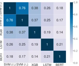
Figure 1: Jaccard similarity between the top 10 fea-tures of different models based on built-in feature im-portance on Yelp. The similarity is the greatest between

SVM (`2) and SVM (`1), while LSTM with attention

and BERT pay attention to quite different features from other models.

planations across models. Third, the similarity

with small k is higher (H1c) because hopefully,

all models and methods agree what the most im-portant features are.

Heterogeneity between instances. Given a pair of (model, method) combinations, our second ques-tion is concerned with how instance-level prop-erties affect the similarity in important features between different combinations. We hypothesize that 1) when two models agree on the predicted label, the similarity between important features is

greater (H2a); 2) longer instances are less likely

to share similar important features (H2b). 3)

in-stances with higher type-token ratio,3which might

be more complex, are less likely to share similar

important features (H2c).

Distribution of important features.Finally, we ex-amine what words tend to be chosen as important features. This question certainly depends on the nature of the task, but we would like to understand how consistent different models and methods are. We hypothesize that 1) deep learning models

gen-erate more diverse important features (H3a); 2)

adjectives are more important in sentiment clas-sification, while pronouns are more important in

deception detection as shown in prior work (H3b).

5 Similarity between Instance-level Feature Importance

We start by examining the overall similarity be-tween different models using different methods. In a nutshell, we compute the average Jaccard

simi-larity of topkfeatures for each pair of(m, h)and

3_{Type-token ratio is defined as the number of unique}

(6)

Similarity comparison between models using the built-in method

1 2 3 4 5 6 7 8 9 10

Number of important features (k) 0.05

0.10 0.15 0.20 0.25 0.30 0.35 0.40

Jaccard

Similar

ity

Random built-in - SVM x XGB built-in - SVM x LSTM built-in - XGB x LSTM

(a) Yelp

1 2 3 4 5

0.10 0.15 0.20 0.25 0.30 0.35 0.40

Jaccard

Similar

ity

(b) SST

1 2 3 4 5 6 7 8 9 10

0.2 0.3 0.4 0.5

Jaccard

Similar

ity

(c) Deception

Comparison between the built-in method and post-hoc methods

1 2 3 4 5 6 7 8 9 10

0.10 0.15 0.20 0.25 0.30 0.35 0.40

Jaccard

Similar

ity

Random SVM x LSTM - built-in SVM x LSTM - LIME SVM x LSTM - SHAP

(d) Yelp

1 2 3 4 5

0.2 0.3 0.4 0.5

Jaccard

Similar

ity

(e) SST

1 2 3 4 5 6 7 8 9 10

0.2 0.3 0.4 0.5

Jaccard

Similar

ity

[image:6.595.72.534.63.357.2]

(f) Deception

Figure 2: Similarity comparison between models with the same method.x-axis represents the number of important

features that we consider, whiley-axis shows the Jaccard similarity.Error bars represent standard error throughout the paper.The top row compares three pairs of models using the built-in method, while the second row compares three methods on SVM and LSTM with attention (LSTM in figure legends always refers to LSTM with attention

in this work). The random line is derived using the average similarity between two random samples ofkfeatures

from 100 draws.

(m0, h0). To facilitate effective comparisons, we

first fix the method and compare the similarity of different models, and then fix the model and com-pare the similarity of different methods. Figure

1 shows the similarity between different models

using the built-in feature importance for the top

10 features in Yelp (k = 10). Consistent with

H1a, SVM (`2) and SVM (`1) are very similar to

each other, and LSTM with attention and BERT clearly lead to quite different top 10 features from the other models. As the number of important

fea-tures (k) can be useful for evaluating the overall

trend, we thus focus on line plots as in Figure2in

the rest of the paper. This heatmap visualization

represents a snapshot fork = 10using the

built-in method. Also, we only built-include SVM (`2) in

the main paper for ease of visualization and some-times refer to it in the rest of the paper as SVM.

No matter which method we use, important fea-tures from SVM and XGBoost are more similar with each other, than with deep learning mod-els (Figure2).First, we compare the similarity of feature importance between different models

us-ing the same method. Usus-ing the built-in method

(first row in Figure2), the solid line (SVM x

XG-Boost) is always above the other lines, usually by a significant margin, suggesting that deep learning models such as LSTM with attention are less simi-lar to traditional models. In fact, the simisimi-larity be-tween XGBoost and LSTM with attention is lower

than random samples for k = 1,2in SST.

Simi-lar results also hold for BERT (see supplementary materials). Another interesting observation is that post-hoc methods tend to generate greater similar-ity than built-in methods, especially for LIME (the dashed line (LIME) is always above the solid line

(built-in) in the second row of Figure2). This is

likely because LIME only depends on the model behavior (i.e., what the model predicts) and does not account for how the model works.

(7)

at-1 2 3 4 5 6 7 8 9 10 Number of important features (k) 0.1

0.2 0.3 0.4 0.5 0.6 0.7

Jaccard

Similar

ity Random

SVM - built-in x LIME SVM - LIME x SHAP SVM - built-in x SHAP XGB - built-in x LIME XGB - LIME x SHAP XGB - built-in x SHAP LSTM - built-in x LIME LSTM - LIME x SHAP LSTM - built-in x SHAP

(a) Yelp

1 2 3 4 5

0.4 0.6 0.8

Jaccard

Similar

ity Random

(b) SST

1 2 3 4 5 6 7 8 9 10

0.2 0.3 0.4 0.5

Jaccard

Similar

ity Random

[image:7.595.75.524.62.191.2]

(c) Deception

Figure 3: Similarity comparison between methods using the same model. The similarity between different methods based on LSTM with attention is generally lower than other methods. Similar results hold for BERT (see the supplementary material).

1 2 3 4 5 6 7 8 9 10

0.20 0.25 0.30 0.35 0.40

Jaccard

Similar

ity

built-in - agree built-in - disagree LIME - agree LIME - disagree SHAP - agree SHAP - disagree

(a) Yelp

1 2 3 4 5

0.2 0.3 0.4 0.5

Jaccard

Similar

ity

(b) SST

1 2 3 4 5 6 7 8 9 10

0.2 0.3 0.4 0.5

Jaccard

Similar

ity

[image:7.595.70.527.250.389.2]

(c) Deception

Figure 4: Similarity between SVM (`2) and LSTM with attention with different methods grouped by whether these two models agree on the predicted label. The similarity is not always greater when they agree on the predicted labels than when they disagree.

1 2 3 4 5 6 7 8 9 10

Number of important features (k)

−0.8

−0.6

−0.4

−0.2

0.0

Spear

man

correlation

(a) Yelp

1 2 3 4 5

−0.7

−0.6

−0.5

−0.4

−0.3

−0.2

−0.1

0.0

Spear

man

correlation

(b) SST

1 2 3 4 5 6 7 8 9 10

−0.8

−0.6

−0.4

−0.2

0.0

Spear

man

correlation

(c) Deception

Figure 5: In most cases, the similarity between feature importance is negatively correlated with length. Here we only show the comparison between different methods based on the same model. Similar results hold for comparison between different models using the same method. For ease of comparison, the gray line marks the

value0. Generally askgrows, relationship becomes even more negatively correlated.

tention, the similarity between feature importance generated by different methods is the lowest, espe-cially comparing LIME with SHAP. Notably, the results are much more cluttered in deception

de-tection. Contrary toH1b, we do not observe that

LIME is more similar to SHAP than built-in. The order seems to depend on both the task and the model: even within SST, the similarity between built-in and LIME can rank as third, second, or

first. In other words, post-hoc methods generate more similar important features when we compare different models, but that is not the case when we fix the model. It is reassuring that that similarity between any pairs is above random, with a sizable margin in most cases (BERT on SHAP is an ex-ception; see supplementary materials).

Relation with k. As the relative order between

[image:7.595.76.522.446.571.2]

(8)

1 2 3 4 5 6 7 8 9 10 Number of important features (k) 3

4 5 6 7 8 9

Entrop

y SVM - built-in_{SVM - LIME}

SVM - SHAP XGB - built-in XGB - LIME XGB - SHAP LSTM - built-in LSTM - LIME LSTM - SHAP

(a) Yelp

1 2 3 4 5

Number of important features (k) 5

6 7 8 9 10

Entrop

(b) SST

1 2 3 4 5 6 7 8 9 10

Number of important features (k) 3

4 5 6 7 8

Entrop

[image:8.595.73.526.62.195.2]

(c) Deception

Figure 6: The entropy of important features. LSTM with attention generates more diverse important features than SVM and XGBoost.

Background SVM XGB LSTM 5.0

7.5 10.0 12.5 15.0 17.5 20.0 22.5

Percentage

NOUN VERB ADJ ADV PRON DET

(a) Yelp

Background SVM XGB LSTM 5

10 15 20 25

Percentage

(b) SST

Background SVM XGB LSTM 0

5 10 15 20 25 30 35 40

Percentage

(c) Deception

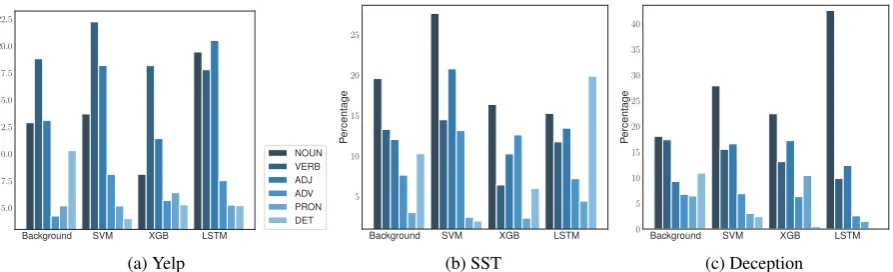
Figure 7: Part-of-speech tag distribution with the built-in method. “Background” shows the distribution of all words in the test set. LSTM with attention puts a strong emphasis on nouns in deception detection, but is not necessarily more different from the background than other models.

so far only focused on relatively consistent

pat-terns over k and classification tasks. Contrary

to H1c, the similarity between most approaches

is not drastically greater for smallk, which

sug-gests that different approaches may not even agree on the most important features. In fact, there is

no consistent trend as kgrows: similarity mostly

increases in SST (while our hypothesis is that it decreases), increases or stays level in Yelp, and shows varying trends in deception detection.

6 Heterogeneity between Instances

Given the overall low similarity between different methods/models, we next investigate how the sim-ilarity may vary across instances.

The similarity between models is not always greater when two models agree on the predicted label (Figure 4). One hypothesis for the over-all low similarity between models is that different models tend to give different predictions therefore they choose different features to support their de-cisions. However, we find that the similarity be-tween models is not particularly high when they agree on the predicted label, and are sometimes

even lower than when they disagree. This is true for LIME in Yelp and for all methods in deception detection. In SST, the similarity when the models agree on the predicted label is generally greater than when they disagree. We show the

compari-son between SVM (`2) and LSTM here, and

simi-lar results hold for other combinations (see supple-mentary materials). This observation suggests that feature importance may not connect with the pre-dicted labels: different models agree for different reasons and also disagree for different reasons.

The similarity between models and methods is generally negatively correlated with length but positively correlated with type-token ratio

(Fig-ure5).Our results supportH2b: Spearman

corre-lation between length and similarity is mostly

be-low0, which indicates that the longer an instance

is, the less similar the important features are. The

negative correlation becomes stronger askgrows,

[image:8.595.80.527.241.377.2]

(9)

1 2 3 4 5 6 7 8 9 10 Number of important features (k) 0.10

0.15 0.20 0.25 0.30 0.35 0.40

Jensen-Shannon

Score _{SVM - built-in x background}

SVM - LIME x background SVM - SHAP x background XGB - built-in x background XGB - LIME x background XGB - SHAP x background LSTM - built-in x background LSTM - LIME x background LSTM - SHAP x background

(a) Yelp

1 2 3 4 5 6 7 8 9 10

0.05 0.10 0.15 0.20 0.25 0.30 0.35

Jensen-Shannon

(b) SST

1 2 3 4 5 6 7 8 9 10

0.2 0.3 0.4 0.5 0.6

Jensen-Shannon

[image:9.595.73.524.61.188.2]

(c) Deception

Figure 8: Distance of the part-of-speech tag distributions between important features and all words (background). Distance is generally smaller with post-hoc methods for all models, although some exceptions exist for LSTM with attention and BERT.

the declining relationship with k does not hold.

Our result on type-token ratio is opposite toH2c:

the greater the type-token ratio, the higher the sim-ilarity (see supplementary materials). We believe that the reason is that type-token ratio is strongly negatively correlated with length (the Spearman correlation for Yelp, SST and deception dataset is -0.92, -0.59 and -0.84 respectively). In other words, type-to-token ratio becomes redundant to length and fails to capture text complexity beyond length.

7 Distribution of Important Features

Finally, we examine the distribution of impor-tant features obtained from different approaches. These results may partly explain our previously observed low similarity in feature importance.

Important features show higher entropy using LSTM with attention and lower entropy with XGBoost (Figure 6). As expected from H3a, LSTM with attention (the pink lines) are usually at the top (similar results for BERT in the supple-mentary material). Such a high entropy can con-tribute to the low similarity between LSTM with attention and other models. However, as the order in similarity between SVM and XGBoost is less stable, entropy cannot be the sole cause.

Distribution of POS tags (Figure7 and Figure

8).We further examine the linguistic properties of

important words. Consistent withH3b, adjectives

are more important in sentiment classification than in deception detection. On the contrary to our hy-pothesis, we found that pronouns do not always play an important role in deception detection. No-tably, LSTM with attention puts a strong empha-sis on nouns in deception detection. In all cases, determiners are under-represented among impor-tant words. With respect to the distance of

part-of-speech tag distributions between important fea-tures and all words (background), post-hoc meth-ods tend to bring important words closer to the background words, which echoes the previous ob-servation that post-hoc methods tend to increase

the similarity between important words (Figure8).

8 Concluding Discussion

In this work, we provide the first systematic char-acterization of feature importance obtained from different approaches. Our results show that ent approaches can sometimes lead to very differ-ent important features, but there exist some con-sistent patterns between models and methods. For instance, deep learning models tend to generate diverse important features that are different from traditional models; post-hoc methods lead to more similar important features than built-in methods.

As important features are increasingly adopted for varying use cases (e.g., decision making vs. model debugging), we hope to encourage more work in understanding the space of important fea-tures, and how they should be used for different purposes. While we focus on consistent patterns across classification tasks, it is certainly interest-ing to investigate how properties related to tasks and data affect the findings. Another promising direction is to understand whether more concen-trated important features (lower entropy) lead to better human performance in supporting decision making.

Acknowledgments

(10)

References

Dzmitry Bahdanau, Kyunghyun Cho, and Yoshua

Ben-gio. 2015. Neural machine translation by jointly

learning to align and translate. In Proceedings of

ICLR.

Tianqi Chen and Carlos Guestrin. 2016. XGBoost: A

scalable tree boosting system. In Proceedings of

KDD.

Jacob Devlin, Ming-Wei Chang, Kenton Lee, and Kristina Toutanova. 2019. Bert: Pre-training of deep bidirectional transformers for language

understand-ing. InProceedings of NAACL.

Finale Doshi-Velez and Been Kim. 2017. Towards a rigorous science of interpretable machine learning.

arXiv preprint arXiv:1702.08608.

Riccardo Guidotti, Anna Monreale, Salvatore Rug-gieri, Franco Turini, Fosca Giannotti, and Dino Pe-dreschi. 2019. A survey of methods for explaining

black box models. ACM computing surveys (CSUR),

51(5):93.

Matthew Honnibal and Ines Montani. 2017. spacy 2: Natural language understanding with bloom embed-dings, convolutional neural networks and incremen-tal parsing.

Benjamin D Horne, Dorit Nevo, John O’Donovan, Jin-Hee Cho, and Sibel Adali. 2019. Rating reliability and bias in news articles: Does ai assistance help

everyone? InProceedings of ICWSM.

Sarthak Jain and Byron C. Wallace. 2019. Attention is

not explanation. InProceedings of NAACL.

Thorsten Joachims. 1998. Text categorization with

support vector machines: Learning with many

rel-evant features. InProceedings of ECML.

Been Kim, Rajiv Khanna, and Oluwasanmi O Koyejo.

2016. Examples are not enough, learn to

criti-cize! criticism for interpretability. InProceedings

of NeurIPS.

Vivian Lai and Chenhao Tan. 2019. On human predic-tions with explanapredic-tions and predicpredic-tions of machine learning models: A case study on deception detec-tion. InProceedings of FAT*.

Jiwei Li, Xinlei Chen, Eduard Hovy, and Dan Jurafsky. 2016. Visualizing and understanding neural models

in nlp. InProceedings of NAACL.

Zachary C Lipton. 2016. The mythos of model

inter-pretability. arXiv preprint arXiv:1606.03490.

Tania Lombrozo. 2012. Explanation and abductive

in-ference. Oxford handbook of thinking and

reason-ing, pages 260–276.

Scott M Lundberg and Su-In Lee. 2017. A unified

ap-proach to interpreting model predictions. In

Pro-ceedings of NeurIPS.

Thang Luong, Hieu Pham, and Christopher D.

Man-ning. 2015. Effective approaches to

attention-based neural machine translation. In Proceedings of EMNLP.

Dmitry M Malioutov, Kush R Varshney, Amin Emad,

and Sanjeeb Dash. 2017. Learning interpretable

classification rules with boolean compressed

sens-ing. InTransparent Data Mining for Big and Small

Data, pages 95–121. Springer.

Dong Nguyen. 2018. Comparing automatic and human evaluation of local explanations for text

classifica-tion. InProceedings of NAACL.

Myle Ott, Claire Cardie, and Jeffrey T Hancock. 2013.

Negative deceptive opinion spam. InProceedings of

NAACL.

Myle Ott, Yejin Choi, Claire Cardie, and Jeffrey T Han-cock. 2011. Finding deceptive opinion spam by any

stretch of the imagination. InProceedings of ACL.

Marco Tulio Ribeiro, Sameer Singh, and Carlos Guestrin. 2016. Why should i trust you?: Explain-ing the predictions of any classifier. InProceedings of KDD.

Sofia Serrano and Noah A. Smith. 2019. Is Attention

Interpretable? InProceedings of ACL.

Avanti Shrikumar, Peyton Greenside, and Anshul

Kun-daje. 2017. Learning important features through

propagating activation differences. InProceedings

of ICML.

Richard Socher, Alex Perelygin, Jean Wu, Jason Chuang, Christopher D Manning, Andrew Ng, and

Christopher Potts. 2013. Recursive deep models

for semantic compositionality over a sentiment

tree-bank. InProceedings of EMNLP.

Ashish Vaswani, Noam Shazeer, Niki Parmar, Jakob Uszkoreit, Llion Jones, Aidan N Gomez, Łukasz Kaiser, and Illia Polosukhin. 2017. Attention is all

you need. InProceedings of NeurIPS.