Better Language Models with Model Merging

(1)

B e t t e r Language M o d e l s with M o d e l Merging

T h o r s t e n B r a n t s

U n i v e r s i t g t d e s S a a r l a n d e s , C o m p u t a t i o n a l L i n g u i s t i c s P . O . B o x 151150, D - 6 6 0 4 1 S a a r b r i i c k e n , G e r m a n y

t h o r s t en@coli, u n i - sb. de

A b s t r a c t

This paper investigates model merging, a technique for deriving Markov models from text or speech corpora. Models are derived by starting with a large and specific model and by successively combining states to build smaller and more general models. We present methods to reduce the time complexity of the algorithm and report on experiments on deriving language models for a speech recognition task. The experiments show the advantage of model merging over the standard bigram approach. The merged model assigns a lower perplexity to the test set and uses consi- derably fewer states.

I n t r o d u c t i o n

Hidden Markov Models are commonly used for statistical language models, e.g. in part-of-speech tagging and speech recognition (Rabiner, 1989). The models need a large set of parameters which are induced from a (text-) corpus. The parameters should be optimal in the sense that the resulting models assign high probabilities to seen training data as well as new data that arises in an applica- tion.

There are several methods to estimate model parameters. The first one is to use each word (type) as a state and estimate the transition probabilities between two or three words by using the relative frequencies of a corpus. This method is commonly used in speech recognition and known as word-bigram or word-trigram model. The relative frequencies have to be smoothed to handle the sparse data problem and to avoid zero probabilities.

T h e second m e t h o d is a variation of the first method. Words are automatically grouped, e.g. by similarity of distribution in the corpus (Pereira et al., 1993). T h e relative frequencies of pairs or triples of groups (categories, clusters) are used as model parameters, each group is represen- ted by a state in the model. The second method

has the advantage of drastically reducing the number of model parameters and thereby reducing the sparse data problem; there is more d a t a per group than per word, thus estimates are more precise.

The third m e t h o d uses manually defined categories. They are linguistically motivated and usually called

parts-of-speech.

An i m p o r t a n t difference to the second m e t h o d with automatically derived categories is that with the manual defini- tion a word can belong to more than one category. A corpus is (manually) tagged with the categories and transition probabilities between two or three categories are estimated from their relative frequencies. This m e t h o d is commonly used for part-of-speech tagging (Church, 1988).

T h e fourth m e t h o d is a variation of the third m e t h o d and is also used for part-of-speech tagging. This m e t h o d does not need a pre-annotated corpus for parameter estimation. Instead it uses a lexicon stating the possible parts-of-speech for each word, a raw text corpus, and an initial bias for the transition and o u t p u t probabilities. T h e parameters are estimated by using the Baum-Welch algorithm (Baum et al., 1970). T h e accuracy of the derived model depends heavily on the initial bias, but with a good choice results are comparable to those of method three (Cutting et al., 1992).

This paper investigates a fifth m e t h o d for esti- mating natural language models, combining the advantages of the methods mentioned above. It is suitable for both speech recognition and part- of-speech tagging, has the advantage of automatically deriving word categories from a corpus and is capable of recognizing the fact t h a t a word belongs to more than one category. Unlike other techniques it not only induces transition and output probabilities, but also the model topology, i.e., the number of states, and for each state the outputs that have a non-zero probability. T h e method is called model merging and was introduced by (Omohundro, 1992).

(2)

dels and present the model merging technique. Then, techniques for reducing the time complexity are presented and we report two experiments using these techniques.

M a r k o v M o d e l s

A discrete output, first order Markov Model consists of

• a finite set of states QU{qs, qe}, q~, qe ~ Q, with q~ the start state, and q~ the end state;

• a finite output alphabet ~;

• a (IQ] + 1) × (IQ] + 1) matrix, specifying the probabilities of state transitions p(q'iq) between states q and q~ (there are no transitions into q~, and no transitions originating in qe); for each state q E Q U {qs}, the sum of the outgoing transition probabilities is 1, ~ p(q']q) =

qlEQU{qe}

1;

• a ]Q] × [~l m a t r i x , specifying the output probabilities p(a]q) of state q emitting output o'; for each state q E Q, the sum of the output probabilities is 1, ~ p(cr]q) = 1.

a E ~

A Markov model starts running in the start state q~, makes a transition at each time step, and stops when reaching the end state qe. The transition from one state to another is done according to the probabilities specified with the transitions. Each time a state is entered (except the start and end state) one of the outputs is chosen (again according to their probabilities) and emitted.

A s s i g n i n g P r o b a b i l i t i e s t o D a t a

For the rest of the paper, we are interested in the probabilities which are assigned to sequences of outputs by the Markov models. These can be calculated in the following way.

Given a model M , a sequence of outputs o = o1 . . . o'k and a sequence of states Q = ql. • • qk (of same length), the probability that the model running through the sequence of states and emitting the given outputs is

(/I

PM(Q, o') = PM(qilqi-1)PM(o'ilqi PM(qelqi)

\i=1

(with q0 = qs). A sequence of outputs can be emitted by more t h a n one sequence of states, thus we have to sum over all sequences of states with the given length to get the probability t h a t a model emits a given sequence of outputs:

PM(O') = ~ PM(Q, o'). Q

The probabilities are calculated very efficiently with the Viterbi algorithm (Viterbi, 1967). Its time complexity is linear to the sequence length despite the exponential growth of the search space.

P e r p l e x i t y

Markov models assign rapidly decreasing probabilities to output sequences of increasing length. To compensate for different lengths and to make their probabilities comparable, one uses the perplexity PP of an output sequence instead of its probability. The perplexity is defined as

1

PPM(O')-

~v/fi ~

The probability is normalized by taking the k th

root (k is the length of the sequence). Similarly, the log perplexity LP is defined:

- log PM

(o')

LPM((r) = log PPM(a) -- k

Here, the log probability is normalized by dividing by the length of the sequence.

PP and LP are defined such t h a t higher perplexities (log perplexities, resp.) correspond to lower probabilities, and vice versa. These mea- sures are used to determine the quality of Markov models. The lower the perplexity (and log perplexity) of a test sequence, the higher its probability, and thus the better it is predicted by the model.

M o d e l M e r g i n g

Model merging is a technique for inducing model parameters for Markov models from a text corpus. It was introduced in (Omohundro, 1992) and (Stolcke and Omohundro, 1994) to induce models for regular languages from a few samples, and adapted to natural language models in (Brants, 1995). Unlike other techniques it not only induces transition and o u t p u t probabilities from the corpus, but also the model topology, i.e., the number of states and for each state the o u t p u t s t h a t have non-zero probability. In n - g r a m approaches the topology is fixed. E.g., in a p o s - n - g r a m model, the states are mostly syntactically motivated, each state represents a syntactic category and only words belonging to the same category have a non-zero o u t p u t probability in a particular state. However the n - g r a m - m o d e l s m a k e the implicit assumption t h a t all words belonging to the same category have a similar distribution in a corpus. This is not true in m o s t of the cases.

(3)

a ) a b

o~ @

'@

c

@

.@

p(SlM~) = ~ ~ 3 . 7 . 1 0 -2

D

.@

b ) b

5 .@

p(SIMb) = ~ --~ 3 . 7 . 1 0 -2

¢)

@

p(SIM~) = ~ -~ 3 . 7 . 1 0 -2

C

, ~ 0.67 , ; @

0.5

d)

@

D

@ 05 . @ ~

0.5

p(SIMd ) = ~ ~_ 1.6-10 -2

"'--@

.

e)

p(SiM~ ) = 2~ ~ 6.6.10 -3 _{4 0 9 6 - -}

b C

o

~ , 0 y

[image:3.612.99.538.78.619.2]

(4)

is that it can recognize t h a t a word (the type) belongs to more than one category, while each occurrence (the token) is assigned a unique category. This naturally reflects manual syntactic categori- zations, where a word can belong to several syntactic classes but each occurrence of a word is un- ambiguous.

The Algorithm

Model merging induces Markov models in the following way. Merging starts with an initial, very general model. For this purpose, the m a x i m u m likelihood Markov model is chosen, i.e., a model t h a t exactly matches the corpus. There is one p a t h for each utterance in the corpus and each p a t h is used by one utterance only. Each p a t h gets the same probability l / u , with u the number of utterances in the corpus. This model is also referred to as the trivial model. Figure 1.a shows the trivial model for a corpus with words a, b, c and utterances ab, ac, abac. It has one p a t h for each of the three utterances ab, ac, and abac, and each p a t h gets the same probability 1/3. The trivial model assigns a probability of p(SIM~ ) = 1/27 to the corpus. Since the model makes an implicit independence assumption between the utterances, the corpus probability is calculated by multiplying the utterance's probabilities, yielding 1 / 3 . 1 / 3 . 1 / 3 = 1/27.

Now states are merged successively, except for the start and end state. Two states are selected and removed and a new merged state is added. T h e transitions from and to the old states are redi- rected to the new state, the transition probabilities are adjusted to maximize the likelihood of the corpus; the o u t p u t s are joined and their probabilities are also adjusted to maximize the likelihood. One step of merging can be seen in figure 1.b. States 1 and 3 are removed, a combined state 1,3 is added, and the probabilities are adjusted.

T h e criterion for selecting states to merge is the probability of the Markov model generating the corpus. We want this probability to stay as high as possible. Of all possible merges (generally, there are k(k - 1)/2 possible merges, with k the n u m b e r of states exclusive start and end state which are not allowed to merge) we take the merge t h a t results in the minimal change of the probability. For the trivial model and u pairwise different utterances the probability is p(SIMtri~) = 1/u ~. T h e probability either stays constant, as in Figure 1.b and c, or decreases, as in 1.d and e. The probability never increases because the trivial model is the m a x i m u m likelihood model, i.e., it maximizes the probability of the corpus given the model.

Model merging stops when a predefined threshold for the corpus probability is reached.

Some statistically m o t i v a t e d criteria for ter- mination using model priors are discussed in (Stotcke and Omohundro, 1994).

Using Model Merging

The model merging algorithm needs several op- timizations to be applicable to large natural language corpora, otherwise the a m o u n t of time needed for deriving the models is too large. Gene- rally, there are O(l 2) hypothetical merges to be tested for each merging step (l is the length of the training corpus). The probability of the training corpus has to be calculated for each hypothetical merge, which is O(l) with d y n a m i c p r o g r a m m i n g . Thus, each step of merging is O(13). If we want to reduce the model from size l 4- 2 (the trivial modeli which consists of one state for each token plus initial and final states) to some fixed size, we need O(l) steps of merging. Therefore, deriving a Markov model by model merging is O(l 4) in time. (Stolcke and Omohundro, 1994) discuss several computational shortcuts and approximati- ons:

1. I m m e d i a t e merging of identical initial and final states of different utterances. These merges do not change the corpus probability and thus are the first merges anyway.

2. Usage of the Viterbi p a t h (best path) only instead of s u m m i n g up all paths to determine the corpus probability.

3. The assumption t h a t all input samples retain their Viterbi p a t h after merging. Making this approximation, it is no longer necessary to re- parse the whole corpus for each hypothetical merge.

We use two additional strategies to reduce the time complexity of the algorithm: a series of cas- caded constraints on the merges and the variation of the starting point.

Constraints

When applying model merging one can observe t h a t first mainly states with the same o u t p u t are merged. After several steps of merging, it is no longer the same output but still mainly states t h a t output words of the same syntactic category are merged. This behavior can be exploited by introducing constraints on the merging process. T h e constraints allow only some of the otherwise possible merges. Only the allowed merges are tested for each step of merging.

(5)

generating the same outputs. If the current model has N states and we divide them into k > 1 non- empty equivalence classes C1 . . . C~, then, instead of N ( N - 1)/2, we have to test

k

.[C'l(IC{l-

])

< N(N

-

1)

2 2

i = 1

merges only.

The best case for a model of size N is the division into N / 2 classes of size 2. Then, only N/2 merges must be tested to find the best merge.

The best division into k > 1 classes for some model of size N is the creation of classes that all have the same size N / k (or an approximation if N / k ~ IN). Then,

N N N(~- - 1)

v ( v - 1 )

. k -

2 2

must be tested for each step of merging.

Thus, the introduction of these constraints does not reduce the order of the time complexity, but it can reduce the constant factor significantly (see section about experiments).

The following equivalence classes can be used for constraints when using untagged corpora:

1. States that generate the same outputs (unigram constraint)

2. unigram constraint, and additionally all prede- cessor states must generate the same outputs (bigram constraint)

3. trigrams or higher, if the corpora are large enough

4. a variation of one: states that output words belonging to one ambiguity class, i.e. can be of a certain number of syntactic classes.

Merging starts with one of the constraints. Af- ter a number of merges have been performed, the constraint is discarded and a weaker one is used instead.

The standard n-gram approaches are special cases of using model merging and constraints. E.g., if we use the unigram constraint, and merge states until no further merge is possible under this constraint, the resulting model is a standard bigram model, regardless of the order in which the merges were performed.

In practice, a constraint will be discarded be- fore no further merge is possible (otherwise the model could have been derived directly, e.g., by the standard n-gram technique). Yet, the que- stion when to discard a constraint to achieve best results is unsolved.

T h e Starting P o i n t

The initial model of the original model merging procedure is the m a x i m u m likelihood or trivial model. This model has the advantage of directly representing the corpus. But its disadvantage is its huge number of states. A lot of computation time can be saved by choosing an initial model with fewer states.

The initial model must have two properties:

1. it must be larger than the intended model, and

2. it must be easy to construct.

The trivial model has both properties. A class of models that can serve as the initial model as well are n-gram models. These models are smaller by one or more orders of magnitude than the trivial model and therefore could speed up the derivation of a model significantly.

This choice of a starting point excludes a lot of solutions which are allowed when starting with the m a x i m u m likelihood model. Therefore, starting with an n-gram model yields a model that is at most equivalent to one that is generated when starting with the trivial model, and that can be much worse. But it should be still better than any n-gram model that is of lower of equal order than the initial model.

E x p e r i m e n t s

M o d e l M e r g i n g vs. B i g r a m s

The first experiment compares model merging with a standard bigram model. Both are trai- ned on the same data. We use Ntra~n -- 14,421

words of the Verbmobil corpus. The corpus

consists of transliterated dialogues on business appointments 1. The models are tested on Ntest = 2,436 words of the same corpus. Training and test parts are disjunct.

The bigram model yields a Markov model wit h 1,440 states. It assigns a log perplexity of 1.20 to the training part and 2.40 to the test part.

Model merging starts with the m a x i m u m likelihood model for the training part. It has 14,423 states, which correspond to the 14,421 words (plus an initial and a final state). The initial log perplexity of the training part is 0.12. This low value shows that the initial model is very specialized in the training part.

(6)

- log]o

P/Ntrain

2 . 5 -

2.0

1 . 5

1 . 0

0 . 5

0 1

I

14

lp

dlp

constraint , t c h a n g ~

I ' I ~ I ' i ' I ; I ' I ' I ' I ' I ' I ' I i I

2 3 4 5 6 7 8 9 10 11 12 13 14 × 1 0 3 merges

I I I I I I i I I I I I I I

13 12 11 10 9 8 7 6 5 4 3 2 1 0 × 1 0 3 states

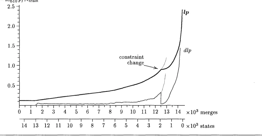
Figure 2: Log Perplexity of the training part during merging. Constraints: same output until 12,500 / none after 12,500. The thin lines show the further development if we retain the the same-output constraint until no further merge is possible. The length of the training part is g t r a i n ---- 14,421.

- log10 p / N t e s t

2 . 8 - 2.77- 2 . 6 - 2 . 5 - 2.4 2 . 3 - 2 . 2 - 0

i

14

I ' I I ' I ' I ' I ' [ ' I '

1 2 3 4 5 6 7 8

I I I I I I I

constraint change

~\%~L~-~lP

/Pbigrara (1440 states)

/Pmin (113 states)

l ' I ' I ' I ' I ' I

9 10 11 12 13 14 xl03 merges

I I i ~ I I

4 3 2 1 0 × 10 3 states 13 12 11 10 9 8 7 6 5

[image:6.612.63.518.94.330.2] [image:6.612.61.525.408.595.2]

(7)

We start merging with the same-output (unigram) constraint to reduce computation time. Af- ter 12,500 merges the constraint is discarded and from then on all remaining states are allowed to merge. The constraints and the point of changing the constraint are chosen for pragmatic reasons. We want the constraints to be as week as possible to allow the maximal number of solutions but at the same time the number of merges must be manageable by the system used for computation (a SparcServerl000 with 250MB main memory). As the following experiment will show, the exact points of introducing/discarding constraints is not i m p o r t a n t for the resulting model.

There are

Ntrain (Nt,ai,~-

1)/2 ~ 10 s hypothetical first merges in the unconstraint case. This number is reduced to --~ 7 . 105 when using the unigram constraint, thus by a factor of .v 150. By using the constraint we need about a week of computation time on a SparcServer 1000 for the whole merging process. Computation would not have been feasible without this reduction.

Figure 2 shows the increase in perplexity during merging. There is no change during the first 1,454 merges. Here, only identical sequences of initial and final states are merged (compare figure 1.a to c). These merges do not influence the probability assigned to the training part and thus do not change the perplexity.

Then, perplexity slowly increases. It can never decrease: the m a x i m u m likelihood model assigns the highest probability to the training part and thus the lowest perplexity.

Figure 2 also shows the perplexity's slope. It is low until about 12,000 merges, then drastically increases. At about this point, after 12,500 merges, we discard the constraint. For this reason, the curve is discontinuous at 12,500 merges. The effect of further retaining the constraint is shown by the thin lines. These stop after t2,983 merges, when all states with the same outputs are merged (i.e., when a bigram model is reached). Merging without a constraint continues until only three states remain: the initial and the final state plus one proper state.

Note that the perplexity changes very slowly for the largest part, and then changes drastically during the last merges. There is a constant phase between 0 and 1,454 merges. Between 1,454 and ~11,000 merges the log perplexity roughly linearly increases with the number of merges, and it explo- des afterwards.

W h a t happens to the test part? Model merging starts with a very special model which then is generalized. Therefore, the perplexity of some ran- dom sample of dialogue data (what the test part is supposed to be) should decrease during merging.

Table 1: Number of states and Log Perplexity for the derived models and an additional, previously test part, consisting of 9,784 words. (a) standard bigram model, (b) constrained model merging (first experiment), (c) model merging starting with a bigram model(second experiment)

(a) (b) (c)

model MM start type bigrams merging with bigrams

states 1,440 113 113

Log P P 2.78 2.41 2.39

This is exactly what we find in the experiment. Figure 3 shows the log perplexity of the test part during merging. Again, we find the disconti- nuity at the point where the constraint is changed. And again, we find very little change in perplexity during about 12,000 initial merges, and large changes during the last merges.

Model merging finds a model with 113 states, which assigns a log perplexity of 2.26 to the test part. Thus, in addition to finding a model with lower log perplexity than the bigram model (2.26 vs. 2.40), we find a model that at the same time has less than 1/10 of the states (113 vs. 1,440).

To test if we found a model t h a t predicts new data better than the bigram model and to be sure that we did not find a model that is simply very specialized to the test part, we use a new, previously unseen part of the Verbmobil corpus. This part consists of 9,784 words. The bigram model assigns a log perplexity of 2.78, the merged model with 113 states assigns a log perplexity of 2.41 (see table 1). Thus, the model found by model merging can be regarded generally better than the bigram model.

I m p r o v e m e n t s

The derivation of the optimal model took about a week although the size of the training part was relatively small. Standard speech applications do not use 14,000 words for training as we do in this experiment, but 100,000, 200,000 or more. It is not possible to start with a model of 100,000 states and to successively merge them, at least it is not possible on today's machines. Each step would require the test of ,~ 10 9 merges.

(8)

- log10

P/Ntrain

2 . 5 -

2 . 0

1.5

1 . 0 0.5 s / J r

10 11 12

I I I

4 3 2

Ip

/

- log10

p/Ntest

2.8

2.7 - --, 2 . 6 - ~ ... ,~ 2 . 5 - '" \

2.4 - z - ~

2 . 3 - 2 . 2 -

' I ' I

10 11 12

I J I

13 14 x 103 merges i i

i i 4 3 2

1 0 × 10 3 states

lpbigram

lpmin

13 14 ×103 merges

I I

1 0 × 103 states

Figure 4: Log Perplexity of training and test parts when starting with a bigram model. T h e starting point is indicated with o, the curves of the previous experiment are shown in thin lines.

This yields a b i g r a m model. The second experiment uses the bigram model with 1,440 states as its starting point and imposes no constraints on the merges. T h e results are shown in figure 4.

We see t h a t the perplexity curves approach very fast their counterparts from the previous experiment. The states differ from those of the previously found model, but there is no difference in the n u m b e r of states and corpus perplexity in the o p t i m a l point. So, one could in fact, at least in the shown case, start with the bigram model without loosing anything. Finally, we calculate the perplexity for the additional test part. It is 2.39, thus again lower t h a n the perplexity of the bigram model (see table 1). It is even slightly lower than in the previous experiment, but most probably due to r a n d o m variation.

T h e derived models are not in any case equivalent (with respect to perplexity), regardless whe- ther we start with the trivial model or the bigram model. We ascribe the equivalence in the experiment to the particular size of the training corpus. For a larger training corpus, the optimal model should be closer in size to the bigram model, or even larger t h a n a bigram model. In such a case starting with bigrams does not lead to an optimal model, and a t r i g r a m model must be used.

C o n c l u s i o n

We investigated model merging, a technique to induce Markov models from corpora.. The original procedure is improved by introducing constraints and a different initial model. The procedures are shown to be applicable to a transliterated speech

corpus. The derived models assign lower perplexities to test d a t a than the standard bigram model derived from the same training corpus. Additio- nally, the merged model was much smaller than the bigram model.

The experiments revealed a feature of model merging t h a t allows for i m p r o v e m e n t of the method's time complexity. There is a large initial part of merges t h a t do not change the model's perplexity w.r.t, the test part, and t h a t do not influence the final o p t i m a l model. T h e t i m e needed to derive a model is drastically reduced by abbre- viating these initial merges. Instead of starting with the trivial model, one can start with a smaller, easy-to-produce model, but one has to ensure t h a t its size is still larger than the o p t i m a l model.

A c k n o w l e d g e m e n t s

I would like to thank Christer Samuelsson for very useful comments on this paper. This work was supported by the Graduiertenkolleg Kognitions- wissenschaft, Saarbriicken.

R e f e r e n c e s

[Bahl et al., 1983] Lalit R. Bahl, Frederick J e l i - nek, and Robert L. Mercer. 1983. A m a x i m u m likelihood approach to continuous speech recognition. I E E E Transactions on Pattern Analy-

sis and Machine Inlelligence, 5(2):179-190.

[image:8.612.64.472.83.276.2]

(9)

chains. The Annals of Methematical Statistics,

41:164-171.

[Brants, 1995] Thorsten Brants. 1995. Estima- ting HMM topologies. In Tbilisi Symposium

on Language, Logic, and Computation, Human

Communication Research Centre, Edinburgh, HCRC/RP-72.

[Church, 1988] Kenneth Ward Church. 1988. A stochastic parts program and noun phrase par- ser for unrestricted text. In Proc. Second Confe- rence on Applied Natural Language Processing,

pages 136-143, Austin, Texas, USA.

[Cutting et al., 1992] Doug Cutting, Julian Ku- piec, Jan Pedersen, and Penelope Sibun. 1992. A practical part-of-speech tagger. In Procee- dings of the 3rd Conference on Applied Natural

Language Processing (ACL), pages 133-140.

[Jelinek, 1990] F. Jelinek. 1990. Self-organized language modeling for speech recognition. In A. Waibel and K.-F. Lee, editors, Readings in

Speech Recognition, pages 450-506. Kaufmann,

San Mateo, CA.

[Omohundro, 1992] S. M. Omohundro. 1992. Best-first model merging for dynamic learning and recognition. In J. E. Moody, S. J. Han- son, and R. P. Lippmann, editors, Advances in

Neural Information Processing Systems 4, pages

958-965. Kaufmann, San Mateo, CA.

[Pereira et al., 1993] Fernando Pereira, Naftali Tishby, and Lillian Lee. 1993. Distributional clustering of english words. In Proceedings of

the 31st ACL, Columbus, Ohio.

[Rabiner, 1989] L. R. Rabiner. 1989. A tutorial on hidden markov models and selected applications in speech recognition. In Proceedings of

the IEEE, volume 77(2), pages 257-285.

[Stolcke and Omohundro, 1994] Andreas Stolcke and Stephen M. Omohundro. 1994. Best-first model merging for hidden markov model induc- tion. Technical Report TR-94-003, Internatio- nal Computer Science Institute, Berkeley, Cali- fornia, USA.

[Viterbi, 1967] A. Viterbi. 1967. Error bounds for convolutional codes and an asymptotically op- timum decoding algorithm. In IEEE Transac-