Global Thresholding and Multiple Pass Parsing

(1)

G l o b a l T h r e s h o l d i n g a n d M u l t i p l e - P a s s Parsing*

Joshua Goodman

Harvard University

40 Oxford St.

Cambridge, MA 02138

[email protected]

Abstract

We present a variation on classic b e a m thresholding techniques t h a t is up to an order of m a g n i t u d e faster t h a n the traditional method, at the same performance level. We also present a new thresholding technique, global thresholding, which, combined with the new b e a m thresholding, gives an additional factor of two improvement, and a novel technique, multiple pass parsing, t h a t can be combined with the others to yield yet another 50% improvement. We use a new search algorithm to simultaneously optimize the thresholding p a r a m e t e r s of the various algorithms.

1 Introduction

In this paper, we examine thresholding techniques for statistical parsers. While there exist theoretically efficient (O (n 3)) algorithms for parsing Probabilistic Context-Free G r a m m a r s ( P C F G s ) and related formalisms, practical parsing algorithms usually make use of pruning techniques, such as b e a m thresholding, for increased speed.

We introduce two novel thresholding techniques, global thresholding and multiple-pass parsing, and one significant variation o n traditional b e a m thresholding. We examine the value of these techniques when used separately, and when combined. In order to examine the combined techniques, we also introduce an algorithm for optimizing the settings *This material is based in part upon work supported by the National Science Foundation under Grant No. IRI-9350192 and a National Science Foundation Grad- uate Student Fellowship. I would also like to thank Michael Collins, Rebecca Hwa, Lillian Lee, Wheeler Ruml, and Stuart Shieber for helpful discussions, and comments on earlier drafts, and the a n o n y m o u s review- ers for their extensive comments.

11

of multiple thresholds. When all three thresholding methods are used together, they yield very significant speedups over traditional b e a m thresholding, while achieving the same level of performance.

We apply our techniques to C K Y chart parsing, one of the most commonly used parsing m e t h o d s in natural language processing. In a C K Y chart parser, a two-dimensional m a t r i x of cells, the chart, is filled in. Each cell in the chart corresponds-to a span of the sentence, and each cell of the chart contains the nonterminals t h a t could generate t h a t span. Cells covering shorter spans are filled in first, so we also refer to this kind of parser as a b o t t o m - u p chart parser.

T h e parser fills in a cell in the chart by examining the nonterminals in lower, shorter cells, and combining these nonterminals according to the rules of the g r a m m a r . T h e more nonterminals there are in the shorter cells, the more combinations of nonterminals the parser must consider.

In some g r a m m a r s , such as P C F G s , probabilities are associated with the g r a m m a r rules. This introduces problems, since in m a n y P C F G s , almost any combination of nonterminals is possible, perhaps with some low probability. T h e large n u m b e r of possibilities can greatly slow parsing. On the other hand, the probabilities also introduce new o p p o r t u - nities. For instance, if in a particular cell in the chart there is some nonterminal t h a t generates the span with high probability, and another t h a t generates t h a t span with low probability, then we can remove the less likely nonterminal from the cell. T h e less likely nonterminal will p r o b a b l y not be p a r t of either the correct parse or the tree returned by the parser, so removing it will do little harm. This technique is called

beam thresholding.

(2)

80

78

76

74

72

70

68

[image:2.612.83.296.75.233.2]

66

...

T : U

/ / / / / /

10O00

Time

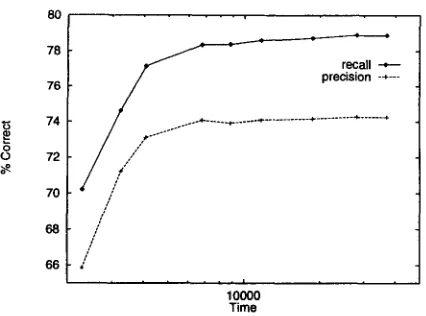
Figure 1: Precision and Recall versus T i m e in B e a m Thresholding

performance measures such as precision and recall will remain virtually unchanged. On the other hand, if we use a tight threshold, removing nonterminals t h a t are almost as probable as the best nonterminal in a cell, then we can get a considerable speedup, but at a considerable cost. Figure 1 shows the tradeoff between accuracy and time.

In this paper, we will consider three different kinds of thresholding. T h e first of these is a variation on traditional b e a m search. In traditional b e a m search, only the probability of a nonterminal generating the terminals of the cell's span is used. We have found t h a t a minor variation, introduced in Section 2, in which we also consider the prior probability t h a t each nonterminal is p a r t of the correct parse, can lead to nearly an order of magnitude improvement.

T h e p r o b l e m with b e a m search is t h a t it only compares nonterminals to other nonterminals in the same cell. Consider the case in which a particular cell contains only b a d nonterminals, all of roughly equal probability. We c a n ' t threshold out these nodes, because even though they are all bad, none is much worse t h a n the best. Thus, what we want is a thresholding technique t h a t uses some global information for thresholding, r a t h e r t h a n just using information in a single cell. T h e second kind of thresholding we consider is a novel technique,

global

thresholding,

described in Section 3. Global thresholding makes use of the observation t h a t for a nonterminal to be p a r t of the correct parse, it must be p a r t of a sequence of reasonably probable nonterminals covering the whole sentence.

T h e last technique we consider,

multiple-pass

parsing,

is introduced in Section 4. T h e basic idea is t h a t we can use information from parsing with one

g r a m m a r to speed parsing with a~other. We run two passes, the first of which is fast and simple, elimi- nating from consideration m a n y unlikely potential constituents. T h e second pass is m o r e complicated and slower, b u t also more accurate. Because we have already eliminated m a n y nodes in our first pass, the second pass can run much faster, and, despite the fact t h a t we have to run two passes, the added sav- ings in the second pass can easily outweigh the cost of the first one.

E x p e r i m e n t a l comparisons of these techniques show t h a t they lead to considerable speedups over traditional thresholding, when used separately. We also wished to combine the thresholding techniques; this is relatively difficult, since searching for the optimal thresholding p a r a m e t e r s in a multi-dimensionai space is potentially very time consuming. We .designed a variant on a gradient descent search algo- r i t h m to find the o p t i m a l p a r a m e t e r s . Using all three thresholding m e t h o d s together, and the p a r a m e t e r search algorithm, we achieved our best results, running an estimated 30 times faster t h a n traditional b e a m search, at the same p e r f o r m a n c e level. 2 B e a m T h r e s h o l d i n g

T h e first, and simplest, technique we will examine is b e a m thresholding. While this technique is used as p a r t of m a n y search algorithms, b e a m thresholding with P C F G s is m o s t similar to b e a m thresholding as used in speech recognition. B e a m thresholding is often used in statistical parsers, such as t h a t of Collins (1996).

Consider a nonterminal X in a cell covering the span of terminals

tj...tk.

We will refer to this as

node

NjXk,

since it corresponds to a potential node in the final parse tree. Recall t h a t in b e a m thresholding, we compare nodes

N~, k

and

N~, k

covering the same span. If one node is much more likely t h a n the other, then it is unlikely t h a t the less p r o b a b l e node will be p a r t of the correct parse, and we can remove it from the chart, saving t i m e later.

There is a subtlety a b o u t w h a t it m e a n s for a node

N~, k

to be more likely t h a n some other node. Ac- cording to folk wisdom, the best way to m e a s u r e the likelihood of a node

N~, k

is to use the probability t h a t the nonterminal X generates the s p a n

tj...tk,

called the

inside probability.

Formally, we write this a s P ( X =~ tj...tk) , and denote it by

~(Nj,k).

x How- ever, this does not give information a b o u t the probability of the node in the context of the full parse tree. For instance, two nodes, one an

NP

and the other a

FRA G

(fragment), m a y have equal inside probabilities, but since there are far more

NPs

t h a n there are

(3)

Therefore, we must consider more information than just the inside probability.

The

outside probability

of a node

N~k

is the prob-

ability of t h a t node given the surrounding terminals of the sentence, i.e.

P(S =~ tl...tj-xXtk+l...tn),

which we denote by

a(N~k ).

Ideally, we would multiply the inside probability by the outside probability, and normalize. This product would give us the overall probability that the node is part of the correct parse. Unfortunately, there is no good way to quickly compute the outside probability of a node during bottom-up chart parsing (although it can be efficiently computed afterwards). Thus, we instead multiply the inside probability simply by the prior probability of the nonterminal type,

P(X),

which is an approximation to the outside probability. Our final thresholding measure is

P(X) xfl(Nj,Xk).

In Sec- tion 7.4, we will show experiments comparing inside- probability beam thresholding to beam thresholding using the inside probability times the prior. Using the prior can lead to a speedup of up to a factor of 10, at the same performance level.

To the best of our knowledge, using the prior probability in beam thresholding is new, although not particularly insightful on our part. Collins (personal communication) independently ob- served the usefulness of this modification, and Caraballo and Charniak (1996) used a related technique in a best-first parser. We think that the main reason this technique was not used sooner is t h a t beam thresholding for P C F G s is derived from beam thresholding in speech recognition using Hid- den Markov Models (HMMs). In an HMM, the forward probability of a given state corresponds to the probability of reaching t h a t state from the start state. The probability of eventually reaching the final state from any state is always 1. Thus, the forward probability is all t h a t is needed. The same is true in some top down probabilistic parsing algorithms, such as stochastic versions of Earley's algorithm (Stolcke, 1993). However, in a bottom-up algorithm, we need the extra factor t h a t indicates the probability of getting from the start symbol to the nonterminal in question, which we approximate by the prior probability. As we noted, this can be very different for different nonterminals.

3 Global T h r e s h o l d i n g

As mentioned earlier, the problem with beam thresholding is t h a t it can only threshold out the worst nodes of a cell. It cannot threshold out an entire cell, even if there are no good nodes in it. To rem- edy this problem, we introduce a novel thresholding technique, global thresholding.

A

B

C

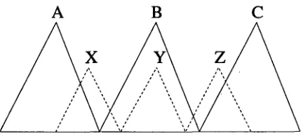
Figure 2: Global Thresholding Motivation

The key insight of global thresholding is due to Rayner and Carter (1996). Rayner et al. noticed t h a t a particular node cannot be part of the correct parse if there are no nodes in adjacent cells. In fact, it must be part of a sequence of nodes stretch- ing from the start of the string to the end. In a probabilistic framework where almost every node will have some (possibly very small) probability, we can rephrase this requirement as being t h a t the node must be part of a reasonably probable sequence.

Figure 2 shows an example of this insight. Nodes A, B, and C will not be thresholded o u t , because each is part of a sequence from the beginning to the end of the chart. On the other hand, nodes X, Y, and Z will be thresholded out, because none is part of such a sequence.

Rayner et al. used this insight for a hierarchical, non-recursive grammar, and only used their technique to prune after the first level of the grammar. They computed a score for each sequence as the minimum of the scores of each node in the sequence, and computed a score for each node in the sequence as the minimum of three scores: one based on statistics about nodes to the left, one based on nodes to the right, and one based on unigram statistics.

We wanted to extend the work of Rayner et al. to general PCFGs, including those t h a t were recursive. Our approach therefore differs from theirs in many ways. Rayner et al. ignore the inside probabilities of nodes; while this may work after processing only the first level of a grammar, when the inside probabilities will be relatively homogeneous, it could cause problems after other levels, when the inside probability of a node will give important information about its usefulness. On the other hand, because long nodes will tend to have low inside probabilities, taking the minimum of all scores strongly favors sequences of short nodes. Furthermore, their algorithm requires time O(n a) t o run just once. This is acceptable if the algorithm is run only after the first level, but running it more often would lead to an overall run time of O(n4). Finally, we hoped to find an algorithm that was somewhat less heuristic in nature.

[image:3.612.310.526.64.161.2]

(4)

f l o a t f [ 1 . . n + l ] := {1,0,0, ...,0}; f o r start := 1 to n

f o r e a c h node N beginning at start left := f [ s t a r t ] ;

score := left × Ninside x Nprior; i f score > f[start + Nlength]

f[start + Ntength] := score;

f l o a t b[1..n+l] := {0, ...,0,0, 1}; f o r start := n downto 1

f o r e a c h node N beginning at start right := b[start + Ntength]; score := right × Ninside × Nprior; i f score > b[start]

b[start] := score; bestProb := f [ n + 1];

f o r e a c h node N left := f[N~t~rt];

right := b[N~t~,rt + Ntenath];

total := left × Ninsid~ X Np~or x right; i f total > bestProb x TG

Nacuve := T R U E ; else

Nacuve := F A L S E ;

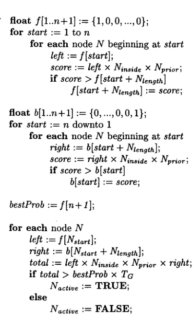
Figure 3: Global Thresholding Algorithm

Our global thresholding technique thresholds out node N if the ratio between the most probable sequence of nodes including node N and the overall most probable sequence of nodes is less t h a n some threshold, To. Formally, denoting sequences of nodes by L, we threshold node N if

TG relax P ( L ) > max P ( L ) LINeL

Now, the hard part is determining P ( L ) , the probability of a node sequence. Unfortunately, there is no way to do this efficiently as part of the intermedi- ate computation of a bottom-up chart parser. 1 We will approximate P ( L ) as follows:

P ( L ) = I I P(LilL1...Li_i) ~ H P(Li)

i i

1Some other parsing techniques, such as stochastic versions of Earley parsers (Stolcke, 1993), efficiently compute related probabilities, but we won't explore these parsers here. We confess that our real interest is in more complicated grammars, such as those that use head words. Grammars such as these can best be parsed bottom up.

T h a t is, we assume independence between the el- ements of a sequence. T h e probability of node Li = N~k is just its prior probability times its inside probability, as before.

The most important difference between global thresholding and beam thresholding is t h a t global thresholding is global: any node in the chart can help prune out any other node. In stark contrast, beam thresholding only compares nodes to other nodes covering the same span. Beam thresholding typically allows tighter thresholds since there are fewer approximations, but does not benefit from global information.

3.1 G l o b a l T h r e s h o l d i n g A l g o r i t h m

Global thresholding is performed in a b o t t o m - u p chart parser immediately after each length is com- pleted. It thus runs n times during the course of parsing a sentence of length n.

We use the simple dynamic programming algorithm in Figure 3. There are O(n 2) nodes in the chart, and each node is examined exactly three times, so the run time of this algorithm is O(n2). T h e first section of the algorithm works forwards, computing, for each i, f[i], which contains the score of the best sequence covering terminals tl...ti-1. Thus f i n + l ] contains the score of the best sequence covering the whole sentence, maxL P(L). T h e algorithm works analogously to the Viterbi algorithm for HMMs. T h e second section is analogous, but works backwards, computing b[i], which contains the score of the best sequence covering terminals ti...tn.

Once we have computed the preceding arrays,

computing

maXL]NE L P ( L ) is straightforward. We simply want the score of the best sequence covering the nodes to the left of N, f[Nstart], times the score of the node itself, times the score of the best sequence of nodes from Ns~art + Nt~ngth to the end, which is just b[N~u, rt + Nt~ngth]. Using this expression, we can threshold each node quickly.

Since this algorithm is run n times during the course of parsing, and requires time O(n 2) each time it runs, the algorithm requires

time O(n 3)

overall. Experiments will show t h a t the time it saves easily outweighs the time it uses.

4 M u l t i p l e - P a s s P a r s i n g

[image:4.612.65.265.62.400.2]

(5)

4.1 Multiple-Pass Speech Recognition

In an idealized multiple-pass speech recognizer, we first run a simple pass, computing the forward and backward probabilities. This first pass runs relatively quickly. We can use information from this simple, fast first pass to eliminate most states, and then run a more complicated, slower second pass t h a t does not examine states t h a t were deemed unlikely by the first pass. T h e e x t r a time of running two passes is more t h a n m a d e up for by the time saved in the second pass.

T h e m a t h e m a t i c s of multiple-pass recognition is fairly simple. In the first simple pass, we record the forward probabilities, c~(S~), and backward probabilities, fl(S~), of each state i at each time t. NOW , ~(s~)×~(s~) gives the overall probability of being in _~(s~,.,) state i at time t given the acoustics. Our second pass will use an H M M whose states are analogous to the first pass H M M ' s states. If a first pass state at some time is unlikely, then the analogous second pass state is p r o b a b l y also unlikely, so we can threshold it out. T h e r e are a few complications to multiple-pass recognition. First, storing all the forward and backward probabilities can be expensive. Second, the second pass is more complicated t h a n the first, typically ineaning t h a t it has more states. So the m a p - ping between states in the first pass and states in the second pass m a y be non-trivial. To solve b o t h these problems, only states at word transitions are saved. T h a t is, from pass to pass, only information a b o u t where words are likely to s t a r t and end is used for thresholding.

4.2 M u l t i p l e - P a s s P a r s i n g

We can use an analogous algorithm for multiple-pass parsing. In particular, we can use two g r a m m a r s , one fast and simple and the other slower, more complicated, and more accurate. R a t h e r t h a n using the forward and backward probabilities of speech recognition, we use the analogous inside and outside probabilities, fl(Nj,k) x and a ( N f k ) respectively. Remem- ber t h a t B(N~i. ) is the probability t h a t N f k is in the correct parse (given, as always, the model and the string). Thus, we run our first pass, computing this expression for each node. We can then eliminate from consideration in our later passes all nodes for which the probability of being in the correct parse was too small in the first pass.

Of course, for our second pass to be more accurate, it will p r o b a b l y be more complicated, typically containing an increased number of nonterminals and productions. Thus, we create a m a p p i n g function

for length := 2 t o n

f o r start := 1 t o n - length + 1 LeftPrev := PrevChart [length][start]; f o r e a c h LeftNodePrev E LeftPrev

f o r e a c h production instance Prod from LeftNodePrev of size length f o r e a c h descendant L of ProdLelt

f o r e a c h descendant R of ProdRight f o r e a c h descendant P of Prodpar~n~

such t h a t P ~ L R add P to Chart[length][start];

Figure 4: Second Pass Parsing Algorithm

from each first pass nonterminal to a set of second pass nonterminals, and threshold out those second pass nonterminals t h a t m a p from low-scoring first pass nonterminals. We call this m a p p i n g function the descendants function. 2

There are m a n y possible examples of first and second pass combinations. For instance, the first pass could use regular nonterminals, such as N P and VP and the second pass could use nonterminals aug- mented with head-word information. T h e descendants function then appends the possible head words to the first pass nonterminals to get the second pass ones.

Even though the correspondence between for- w a r d / b a c k w a r d and inside/outside probabilities is very close, there are i m p o r t a n t differences between speech-recognition HMMs and natural-language processing P C F G s . In particular, we have found t h a t it is more i m p o r t a n t to threshold productions t h a n nonterminals. T h a t is, r a t h e r t h a n just notic- ing t h a t a particular nonterminal VP spanning the words "killed the rabbit" is v e r y likely, we also note t h a t the production VP --~ V N P (and the relevant spans) is likely.

Both the first and second pass parsing algorithms are simple variations on C K Y parsing. In the first pass, we now keep track of each production instance associated with a node, i.e. N'x~,3

~ NYi,k gZk+l,j,

computing the inside and outside probabilities of each. T h e second pass requires more changes. Let us denote the descendants of nonterminal X by X1...Xx. In the second pass, for each production 2In thin paper, we will assume that each second pass nonterminal can descend from at most one first pass nonterminal in each cell. Th~ grammars used here have this property. If this assumption is violated, multiple-pass parsing is still possible, but some of the algorithms need to be changed.

(6)

of the form N. X. ~,~ ~ N Y i,k N~+Ij z in the first pass t h a t wasn't thresholded out by multi-pass thresholding, b e a m thresholding, etc., we consider every descendant production instance, t h a t is, all those of the

Z .

form N~,~ p ~ Ni, ~ N ~ + , j , for a p p r o p r i a t e values of p, q, r. This algorithm is given in Figure 4, which uses a current pass m a t r i x Chart to keep track of nonterminals in the current pass, and a previous pass matrix, PrevChart to keep track of nonterminals in the previous pass. We use one additional optimization, keeping track of the descendants of each nonterminal in each cell in PrevChart which are in the corresponding cell of Chart.

We tried multiple-pass thresholding in two different ways. In the first technique we tried, production- instance thresholding, we remove from consideration in the second pass the descendants of all production instances whose combined inside-outside probability falls below a threshold. In the second technique, node thresholding, we remove from consideration the descendants of all nodes whose inside-outside probability falls below a threshold. In our pilot experiments, we found t h a t in some cases one technique works slightly better, and in some cases the other does. We therefore ran our experiments using b o t h thresholds together.

One nice feature of multiple-pass parsing is t h a t under special circumstances, it is an admissible

search technique, meaning t h a t we are guaranteed to find the best solution with it. In particular, if we parse using no thresholding, and our g r a m m a r s have the p r o p e r t y t h a t for every non-zero probability parse in the second pass, there is an analogous non-zero probability parse in the first pass, then multiple-pass search is admissible. Under these circumstances, no non-zero probability parse will be thresholded out, b u t m a n y zero probability parses m a y be removed from consideration. While we will almost always wish to parse using thresholds, it is nice to know t h a t multiple-pass parsing can be seen as an a p p r o x i m a t i o n to an admissible technique, where the degree of a p p r o x i m a t i o n is controlled by the thresholding p a r a m e t e r .

5 M u l t i p l e P a r a m e t e r

O p t i m i z a t i o n

T h e use of any one of these techniques does not exclude the use of the others. There is no reason t h a t we cannot use b e a m thresholding, global thresholding, and multiple-pass parsing all at the same time. In general, it wouldn't m a k e sense to use a technique such as multiple-pass parsing without other thresholding techniques; our first pass would be overwhelmingly slow without some sort of thresh-

w h i l e n o t Thresholds E ThresholdsSet

add Thresholds to ThresholdsSet;

( BaseET , Base Time ) := ParseAll( Thresholds );

f o r e a c h Threshold E Thresholds

if BaseET >

TargetET

tighten Threshold;

( NewET , New Time ) :-- ParseAll(Thresholds);

Ratio := (BaseTime - NewTime) / (BaseET - NewET);

e l s e

loosen Threshold;

( NewET , New Tim e) := ParseAll (Thresholds);

Ratio := (BaseET - NewET) / (BaseTime - NewTime);

change Threshold with best Ratio;

Figure 5: Gradient Descent Multiple Threshold Search

•

r e s h 2

. . . Goal

Time Optimizing for L o w e r E n t r o p y :

Steeper

is Better

. . . Goal

T h r o b

2 ~ e s h 1

Time Optimizing for

Faster

S p e e d :

Flatter

is B e t t e r Figure 6: Optimizing for Lower E n t r o p y versus Op- timizing for Faster Speed

olding.

There are, however, some practical considerations. To optimize a single threshold, we could simply sweep our p a r a m e t e r s over a one dimensional range, and pick the best speed versus p e r f o r m a n c e tradeoff. In combining multiple techniques, we need to find optimal combinations of thresholding p a r a m e - ters. R a t h e r t h a n having to examine 10 values in a single dimensional space, we might have to examine 100 combinations in a two dimensional space. Later, we show experiments with up to six thresholds. Since we d o n ' t have time to parse with one million p a r a m e t e r combinations, we need a b e t t e r search algorithm.

[image:6.612.320.537.318.452.2]

(7)

achieving t h a t performance level as quickly as possible. If this is our goal, then a normal gradient descent technique w o n ' t work, since we can't use such a technique to optimize one function of a set of variables (time as a function of thresholds) while holding another one constant (performance). 3

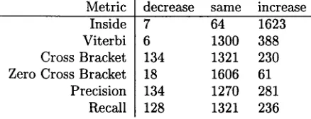
We wanted a metric of performance which would be sensitive to changes in threshold values. In particular, our ideal metric would be strictly increasing as our thresholds loosened, so that every loosening of threshold values would produce a measurable increase in performance. The closer we get to this ideal, the fewer sentences we need to test during parameter optimization.

We tried an experiment in which we ran beam thresholding with a tight threshold, and then a loose threshold, on all sentences of section 0 of length < 40. For this experiment only, we discarded those sentences which could not be parsed with the spec- ified setting of the threshold, rather than retrying with looser thresholds. We then computed for each of six metrics how often the metric decreased, stayed the same, or increased for each sentence between the two runs. Ideally, as we loosened the "threshold, every sentence should improve on every metric, but in practice, ,that wasn't the case. As can be seen, the inside score was by far the most nearly strictly increasing metric. Therefore, we should use the inside probability as our metric of performance; however inside probabilities can become very close to zero, so instead we measure entropy, the negative logarithm of the inside probability.

Metric Inside Viterbi Cross Bracket Zero Cross Bracket Precision Recall

decrease same increase

7 64 1623

6 1300 388

134 1321 230

18 1606 61

134 1270 281

128 1321 236

We implemented a variation on a steepest descent search technique. We denote the entropy of the sentence after thresholding by ET. Our search engine is given a target performance level ET to search for,

3We could use gradient descent to minimize a weighted sum of time and performance, but we wouldn't know at the beginning what performance we would have at the end. If our goal is to have the best performance we can while running in real time, or to achieve a minimum acceptable performance level with as little time as nec- essary, then a simple gradient descent function wouldn't work as well as our algorithm.

Also, for this algorithm (although not for most experiments), our measurement of time was the total number of productions searched, rather than cpu time; we wanted the greater accuracy of measuring productions.

and then tries to find the best combination of parameters that works at approximately this level of performance. At each point, it finds the threshold to change that gives the most "bang for the buck." It then changes this parameter in the correct direction to move towards ET (and possibly overshoot it). A simplified version of the algorithm is given in Figure 5.

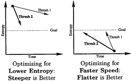
Figure 6 shows graphically how the algorithm works. There are two cases. In the first case, if we are currently above the goal entropy, then we loosen our thresholds, leading to slower speed and lower entropy. We then wish to get as much entropy reduction as possible per time increase; t h a t is, we want the steepest slope possible. On the other hand, if we are trying to increase our entropy, we want as much time decrease as possible per entropy increase; that is, we want the flattest slope possible. Because of this difference, we need to compute different ratios depending on which side of the goal we axe on.

There are several subtleties when thresholds are set very tightly. When we fail to parse a sentence because the thresholds are too tight, we retry the parse with lower thresholds. This can lead to condi- tions that are the opposite of what we expect; for instance, loosening thresholds may lead to faster parsing, because we d o n ' t need to parse the sentence, fail, and then retry with looser thresholds. The full algorithm contains additional checks t h a t our thresholding change had the effect we expected (either increased time for decreased entropy or vice versa). If we get either a change in the wrong direction, or a change that makes everything worse, then we retry with the inverse change, hoping t h a t t h a t will have the intended effect. If we get a change t h a t makes both time and entropy better, then we make that change regardless of the ratio.

Also, we need to do checks t h a t the denominator when computing Ratio isn't too small. If it is very small, then our estimate may be unreliable, and we d o n ' t consider changing this parameter. Finally, the actual algorithm we used also contained a simple "annealing schedule", in which we slowly decreased the factor by which we changed thresholds. T h a t is, we actually run the algorithm multiple times to termination, first changing thresholds by a factor of 16. After a loop is reached at this factor, we lower the factor to 4, then 2, then 1.414, then 1.15.

Note that this algorithm is fairly domain inde- • pendent. It can be used for almost any statistical parsing formalism that uses thresholds, or even for speech recognition.

[image:7.612.82.301.452.536.2]

(8)

6 C o m p a r i s o n to P r e v i o u s Work

Beam thresholding is a common approach. While we don't know of other systems that have used exactly our techniques, our techniques are cer- tainly similar to those of others. For instance, Collins (1996) uses a form of beam thresholding t h a t differs from ours only in that it doesn't use the prior probability of nonterminals as a factor, and Caraballo and Charniak (1996) use a version with the prior, but with other factors as well.

Much of the previous related work on thresholding is in the similar area of priority functions for agenda-based parsers. These parsers t r y to do "best first" parsing, with some function akin to a thresholding function determining what is best. The best comparison of these functions is due to Caraballo and Charniak (1996; 1997), who tried various pri- oritization methods. Several of their techniques are similar to our beam thresholding technique, and one of their techniques, not yet published (Caraballo and Charniak, 1997), would probably work better.

T h e only technique t h a t Caraballo and Charniak (1996) give that took into account the scores of other nodes in the priority function, the "prefix model," required O(n 5) time to compute, compared to our O(n 3) system. On the other hand, all nodes in the agenda parser were compared to all other nodes, so in some sense all the priority functions were global. Note t h a t agenda-based P C F G parsers in general require more than O(n 3) run time, because, when b e t t e r derivations are discovered, they may be forced to propagate improvements to productions t h a t they have previously considered. For instance, if an agenda-based system first computes the probability for a production S ~ NP VP, and then later computes some better probability for the NP, it must u p d a t e the probability for the S as well. This could propagate through much of the chart. To rem- edy this, Caraballo et al. only propagated probabilities t h a t caused a large enough change (Caraballo and Charniak, 1997). Also, the question of when an agenda-based system should stop is a little discussed issue, and difficult since there is no obvious stopping criterion. Because of these issues, we chose not to implement an agenda-based system for comparison. As mentioned earlier, Rayner and Carter (1996) describe a system t h a t is the inspiration for global thresholding. Because of the limitation of their system to non-recursive grammars, and the other differences discussed in Section 3, global thresholding represents a significant improvement.

Collins (1996) uses two thresholding techniques. T h e first of these is essentially beam thresholding

for e a c h rule P ~ L R

i f nonterminal L in left cell i f nonterminal R in right cell

add P to parent cell; Algorithm One

for e a c h nonterminal L in left cell

f o r e a c h ' n o n t e r m i n a l R in right cell

f o r e a c h rule P ~ L R add P to parent cell; Algorithm Two

Figure 7: Two Possible CKY inner loops

without a prior. In the second technique, there is a constant probability threshold. Any nodes with a probability below this threshold are pruned. If the parse fails, parsing is restarted with the constant lowered. We a t t e m p t e d to duplicate this technique, but achieved only negligible performance improvements. Collins (personal communication) re- ports a 38% speedup when this technique is combined with loose beam thresholding, compared to loose beam thresholding alone. Perhaps our lack of success is due to differences between our grammars, which are fairly different formalisms. When Collins began using a formalism somewhat closer to ours, he needed to change his beam thresholding to take into account the prior, so this is not unlikely. Hwa (personal communication) using a model similar to PCFGs, Stochastic Lexicalized Tree Insertion Gram- mars, also was not able to obtain a speedup using this technique.

There is previous work in the speech recognition community on automatically optimizing some parameters (Schwartz et al., 1992). However, this previous work differed significantly from ours b o t h in the techniques used, and in the parameters optimized. In particular, previous work focused on optimizing weights for various components, such as the language model component. In contrast, we optimize thresholding parameters. Previous techniques could not be used or easily adapted to thresholding parameters.

7 E x p e r i m e n t s

7.1 T h e P a r s e r a n d D a t a

(9)

Original

S

X Y

A B ... G H Z

A B

Binary Branching S

X y

A X~,C,D,E,F Z

A B

B XC,D,E,F, G

I

C X D , E , F , G , H

D X ~ _E,F,G,H

E X~,a, H

F X~, H

G H

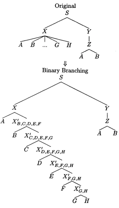
Figure 8: Converting to Binary Branching

added to the parent, can be written in several different ways. Which way this is done interacts with thresholding techniques. There are two possibilities, as shown in Figure 7. We used the second technique, since the first technique gets no speedup from most thresholding systems.

All experiments were trained on sections 2-18 of the Penn Treebank, version II. A few were tested, where noted, on the first 200 sentences of section 00 of length at most 40 words. In one experiment, we used the first 15 ()f length at most 40, and in the re- mainder of our experiments, we used those sentences in the first 1001 of length at most 40. Our parameter optimization algorithm always used the first 31 sentences of length at most 40 words from section 19. We ran some experiments on more sentences, but there were three sentences in this larger test set that could not be parsed with beam thresholding, even with loose settings of the threshold; we therefore chose to report the smaller test set, since it is difficult to compare techniques which did not parse

exactly the same sentences.

7.2 T h e G r a m m a r

We needed several grammars for our experiments so that we could test the multiple-pass parsing algorithm. The g r a m m a r rules, and their associated probabilities, were determined by reading them off of the training section of the treebank, in a man- ner very similar to that used by Charniak (1996). The main grammar we chose was essentially of the following form:

!

X =v A XB,C,D,E, F _! X~,B,C,D~ ~ A XB,c,D,E,F

A X ~ A B

T h a t is, our g r a m m a r was binary branching ex- cept that we also allowed unary branching productions. There were never more than five subscripted symbols for any nonterminal, although there could be fewer than five if there were fewer t h a n five symbols remaining on the right hand sine. Thus, our g r a m m a r was a kind of 6-gram model on symbols in the g r a m m a r : Figure 8 shows an example of how we converted trees to binary branching with our grammar. We refer to this g r a m m a r as the 6-gram grammar. The terminals of the g r a m m a r were the part-of-speech symbols in the treebank. Any experiments that d o n ' t mention which g r a m m a r we used were run with the 6-gram grammar.

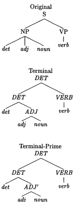
For a simple grammar, we wanted something t h a t would be very fast. The fastest g r a m m a r we can think of we call the terminal grammar, because it has one nonterminal for each terminal symbol in the al- phabet. The nonterminal symbol indicates the first terminal in its span. The parses are binary branching in the same way t h a t the 6-gram g r a m m a r parses are. Figure 9 shows how to convert a parse tree to the terminal grammar. Since there is only one nonterminal possible for each Cell of the chart, parsing is quick for this grammar. For technical and practical reasons, we actually wanted a marginally more complicated grammar, which included the "prime" symbol of the 6-gram grammar, indicating that a cell is part of the same constituent as its parent. Therefore, we doubled the size of the g r a m m a r so that there would be both primed and non-primed

aWe have skipped over details regarding our handling of unary branching nodes. Unary branching nodes are in general difficult to deal with (Stolcke, 1993). The actual gatammars we used contained additional symbols in such a way that there could not be more than one unary branch in a row. This greatly simplified computations, especially of the inside and outside probabilities. We also doubled the number of cells in our parser, having both unary and binary cells for each length/start pair.

[image:9.612.73.272.69.416.2]

(10)

Original S

NP VP

verb det adj noun

Terminal

D E T

D E T V E R B

det A D J verb

adj noun

T e r m i n a l - P r i m e

D E T

D E T V E R B

det A D J ~ verb

adj n o u n

Figure 9: Converting to Terminal and Terminal- P r i m e G r a m m a r s

versions of each terminal; we call this the terminal- prime g r a m m a r , and also show how to convert to it in Figure 9. This is the g r a m m a r we actually used as the first pass in our multiple-pass parsing experiments.

7.3 W h a t w e m e a s u r e d

T h e goal of a good thresholding algorithm is to trade off correctness for increased speed. We must thus measure b o t h correctness and speed, and there are some subtleties to measuring each.

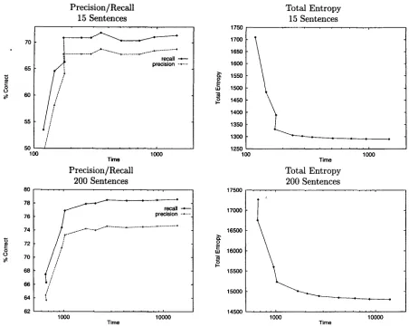
First, the traditional way of measuring correctness is with metrics such as precision and recall. Unfortu- nately, there are two problems with these measures. First, they are two numbers, neither useful without the other. Second, they are subject to considerable noise. In pilot experiments, we found t h a t as we changed our thresholding values monotonically, precision and recall changed non-monotonically (see Figure 11). We a t t r i b u t e this to the fact t h a t we m u s t choose a single parse from our parse forest, and, as we tighten a thresholding p a r a m e t e r , we m a y

threshold out either good or b a d parses. Further- more, rather t h a n just changing precision or recall by a small amount, a single thresholded item m a y completely change the shape of the resulting tree. Thus, precision and recall are only s m o o t h with very large sets of test data. However, because of the large n u m b e r of experiments we wished to run, using a large set of test d a t a was not feasible. Thus, we looked for a surrogate measure, and decided to use the total inside probability of all parses, which, with no thresholding, is just the probability of the sentence given the model. If we denote the t o t a l inside probability with no thresholding by I a n d the total inside probability with thresholding by IT, then /~= is the probability t h a t we did not threshold out the correct parse, given the model. Thus, maximiz- ing IT should maximize correctness. Since probabilities can become very small, we instead minimize entropies, the negative logarithm of the probabilities. Figure 11 shows t h a t with a large d a t a set, entropy correlates well with precision and recall, and t h a t with smaller sets, it is much smoother. E n t r o p y is smoother because it is a function of m a n y more variables: in one experiment, there were a b o u t 16000 constituents which contributed to precision a n d recall measurements, versus 151 million productions potentially contributing to entropy. Thus, we choose entropy as our measure of correctness for m o s t experiments. W h e n we did measure precision and recall, we used the metric as defined by Collins (1996).

Note t h a t the fact t h a t entropy changes s m o o t h l y and monotonically is critical for the p e r f o r m a n c e of the multiple p a r a m e t e r optimization algorithm. Fur- thermore, we m a y have to run quite a few iterations of t h a t algorithm to get convergence, so the fact t h a t entropy is smooth for relatively small n u m b e r s of sentences is a large help. Thus, the discovery t h a t entropy is a good surrogate for precision and recall is non-trivial. T h e same kinds of observations could be extended to speech recognition to optimize multiple thresholds there (the typical m o d e r n speech system has quite a few thresholds), a topic for future research.

Note t h a t for some sentences, with t o o tight thresholding, the parser will fail to find any parse at all. We dealt with these cases by restarting the parser with all thresholds lowered by a factor of 5, iterating this loosening until a parse could be found. This is why for some tight thresholds, the parser m a y be slower t h a n with looser thresholds: the sentence has to be parsed twice, once with tight thresholds, and once with loose ones.

[image:10.612.121.241.69.395.2]

(11)

le+07

0

,0'0o 20'00 30'00 40'00 s0'00 80'0o 70'0o 80 0 9g00,0o0o

Time

6e+07

5e+07

4e+07

~ ~+07 2 a.

2e+07

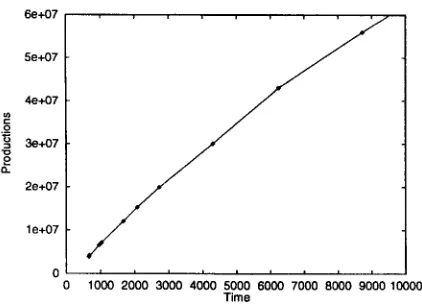
Figure 10: Productions versus T i m e

done by the parser, and elapsed time. If we measure a m o u n t of work done by the parser in terms of the n u m b e r of productions with non-zero probability examined by the parser, w e ' h a v e a fairly implementation-independent, machine-independent measure of speed. On the other hand, because we used m a n y different thresholding algorithms, some with a fair a m o u n t of overhead, this measure seems inappropriate. Multiple-pass parsing requires use of the outside algorithm; global thresholding uses its own dynamic p r o g r a m m i n g algorithm; and even b e a m thresholding has some per-node overhead. Thus, we will give most measurements in terms of elapsed time, not including loading the g r a m m a r and other O(1) overhead. We did want to verify t h a t elapsed time was a reasonable measure, so we did a b e a m thresholding experiment to make sure t h a t elapsed time and n u m b e r of productions examined were well correlated, using 200 sentences and an ex- ponential sweep of the thresholding parameter. T h e results, shown in Figure 10, clearly indicate t h a t time is a good proxy for productions examined.

7.4 Experiments in Beam Thresholding

Our first goal was to show t h a t entropy is a good surrogate for precision and recall. We thus tried two experiments: one with a relatively large test set of 200 sentences, and one with a relatively small test set of 15 sentences. Presumably, the 200 sentence test set should be much less noisy, and fairly indicative of performance. We graphed b o t h precision and recall, and entropy, versus time, as we swept the thresholding p a r a m e t e r over a sequence of values. The results are in Figure 11. As can be seen, entropy is significantly s m o o t h e r t h a n precision and recall for b o t h size test corpora.

Our second goal was to check t h a i the prior probability is indeed helpful. We ran two experiments,

one with the prior and one without. Since the experiments without the prior were much worse t h a n those with it, all other b e a m thresholding experiments included the prior. T h e results, shown in Figure 12, indicate t h a t the prior is a critical component. This experiment was run on 200 sentences of test data.

Notice t h a t as the time increases, the d a t a tends to approach an asymptote, as shown in the left hand graph of Figure 12. In order to m a k e these small a s y m p t o t i c changes more clear,-we wished to ex- pand the scale towards the a s y m p t o t e . T h e right hand graph was plotted with this expanded scale, based on l o g ( e n t r o p y - a s y m p t o t e ) , a slight variation on a normal log scale. We use this scale in all the remaining entropy graphs. A normal logarithmic scale is used for the time axis. T h e fact t h a t the time axis is logarithmic is especially useful for determining how much more efficient one algorithm is t h a n another at a given performance level. If one picks a performance level on the vertical axis, then the distance between the two curves at t h a t level represents the ratio between their speeds. There is roughly a factor of 8 to 10 difference between using the prior and not using it at all graphed performance levels, with a slow trend towards smaller differences as the thresholds are loosened.

7.5 Experiments in Global Thresholding

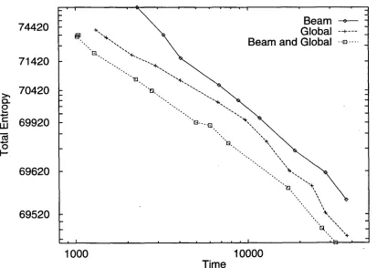
We tried experiments comparing global thresholding to b e a m thresholding. Figure 13 shows the results of this experiment, and later experiments. In the best case, global thresholding works twice as well as b e a m thresholding, in the sense t h a t to achieve the same level of performance requires only half as much time, although smaller improvements were more typical.

We have found that, in general, global thresholding works better on simpler g r a m m a r s . In some complicated g r a m m a r s we explored in other work, there were systematic, strong correlations between nodes, which violated the independence approximation used in global thresholding. This prevented us from using global thresholding with these g r a m m a r s . In the future, we m a y modify global thresholding to model some of these correlations.

7.6 Experiments combining Global

Thresholding and B e a m Thresholding

V(hile global thresholding works b e t t e r t h a n b e a m thresholding in general, each has its own strengths. Global thresholding can threshold across cells, b u t because of the approximations used, the thresholds must generally be looser. B e a m thresholding can only threshold within a cell, but can do so fairly tightly. Combining the two offers the potential to

[image:11.612.75.286.64.217.2]

(12)

70

65

60

55

50 100

80

78

76

74

72

70

68

66

64

62

Precision/Recall

15 Sentences

recall precision -+--*

/

1 0 0 0

Time

Precision/Recall

200 Sentences

i i * .-e

recall precision -~---

/

. . . . i . . . ,

1 000 10050

Time

1750

Total E n t r o p y 15 Sentences 1700

1650

1600

~. 1550 2

1500

1450

1400

1350

1300

1250 100

17500

17000

165OO

o

16000

I

\

15500

15000

14500

, , , , , , i

1000 Time

Total E n t r o p y 200 Sentences

, , , , i , , , , , , , i

1000 10000

Time

Figure 11: Smoothness for Precision and Recall versus Total Inside for Different Test D a t a Sizes

2

17500 ... • . . . . . . . . .

17000 1 \

16500

16000

15500

15000

14500 . . . ' . . .

1000 10000

Time X axis: log(time)

Y axis: entropy

Prior No Prior -+--

\

i i

16786

15786

15286

2

1 4 9 8 6

14886

14836

14806

\ Prior - - ~ ",~ No Prior -~---

!

" x

",\÷

10000 Time

X axis:

log(time)

Y axis: log(entropy - asymptote)

1 0 0 0

[image:12.612.81.533.82.443.2] [image:12.612.85.532.499.677.2]

(13)

o

ILl

0

I--

7 4 4 2 0

7 1 4 2 0

7 0 4 2 0

6 9 9 2 0

6 9 6 2 0

6 9 5 2 0

\

B e a m o

% ~

Global

- + ....

,,., . B e a m and Global --a ....

"El.

"'-,.~..

""El

""~.

• . . . ~

, I , , , , , • ~ , " ~ •

0 0 0 1 0 0 0 0

Time

Figure 13: Combining B e a m and Global Search

get the advantages of both. We ran a series of experiments using the thresholding optimization algorithm of Section 5. Figure 13 gives the results. T h e combination of b e a m and global thresholding together is clearly b e t t e r t h a n either alone, in some cases running 40% faster t h a n global thresholding alone, while achieving the same performance level. The combination generally runs twice as fast as b e a m thresholding alone, although up to a factor of three.

7.7

Experiments in Multiple-Pass Parsing

Multiple-pass parsing improves even further on our experiments combining b e a m and global thresholding. Note t h a t we used b o t h b e a m and global thresholding for b o t h the first and second pass in these experiments. T h e first pass g r a m m a r was the very simple terminal-prime g r a m m a r , and the second pass g r a m m a r was the usual 6-gram g r a m m a r .

We evaluated multiple-pass parsing slightly dif- ferently from the other thresholding techniques. In the experiments conducted here, our first and second pass g r a m m a r s were very different from each other. For a given parse to be returned, it must be in the intersection of b o t h g r a m m a r s , and reasonably likely according to both. Since the first and

second pass g r a m m a r s capture different information, parses which are likely according to b o t h are especially good. T h e entropy of a sentence measures its likelihood according to the second pass, but ig- nores the fact t h a t the returned parse m u s t also be likely according to the first pass. Thus, entropy, our measure in the previous experiments, which measures only likelihood according to the final pass, is not necessarily the right measure to use. We therefore give precision and recall results in this section. We still optimized our thresholding p a r a m e t e r s using the same 31 sentence held out corpus, and min- imizing entropy versus n u m b e r of productions, as before.

We should note t h a t when we used a first pass g r a m m a r t h a t captured a strict subset of the information in the second pass g r a m m a r , we have found t h a t entropy is a very good measure of performance. As in our earlier experiments, it tends to be well correlated with precision and recall b u t less subject to noise. I t is only because of the g r a m m a r m i s m a t c h t h a t we have changed the evaluation.

Figure 14 shows precision and recall curves for single pass versus multiple pass experiments. As in the entropy curves, we can determine the performance

[image:13.612.77.490.67.361.2]

(14)

8 0

"U

(1)

o

O

~e

7 9

7 8

7 7

7 6

7 5

[- : , * * "

i o ' "

.B°°

: . , - °

, ' ]

• '/ /

7 4 I _{i pl tS}~ "

7 3

7 2

... :..-X- ... "X-

... . x ' " ' " ' ] ~ . . . . . - . . B - - - - " : - " : ' - " - - : ' - " : - " : ' - " - " : ' : ' : ' : ' : ' : ' : ' : ' ~ - . x

... . ~ ( ... , , * ""EJ" ° "

x ..'"'" "'~'" B e a m R e c a l l o

~.--" G l o b a l R e c a l l - + ....

./"

B e a m a n d G l o b a l R e c a l l --E~ ....

./"

M u l t i - P a s s R e c a l l ~ ... "

//

B e a m P r e c i s i o n - ~ ....

,//

G l o b a l P r e c i s i o n -~ ....

f B e a m a n d G l o b a l P r e c i s i o n --~ ....

M u l t i - P a s s P r e c i s i o n --+ ...

..-4..- . . .

. . . + . . . + . . . .v;g,.,~, . . . . . . . + - - . ~ . . ~ - - ' ~ . . . ~ . . . . : : ~ . : . ~ _ ~ : . ~ : = = ~ . . . ~,---2,.+

.-"" . . . . 2;:" ... ~ ... --- :~"

/ .r ,r

,/ .i

./ p.~

1 0 0 0 0 T i m e

Figure 14: Multiple Pass Parsing vs. Beam and Global vs. Beam

ratio by looking across horizontally. For instance, the multi-pass recognizer achieves a 74% recall level using 2500 seconds, while the best single pass algorithm requires about 4500 seconds to reach that level. Due to the noise resulting from precision and recall measurements, it is hard to exactly quantify the advantage from multiple pass parsing, but it is generally about 50%.

8 A p p l i c a t i o n s and C o n c l u s i o n s

8.1 A p p l i c a t i o n to O t h e r F o r m a l i s m s

In this paper, we only considered applying multiple- pass and global thresholding techniques to parsing probabilistic context-free grammars. However, just about any probabilistic grammar formalism for which inside and outside probabilities can be computed can benefit from these techniques. For instance, Probabilistic Link Grammars (Lafferty, Sleator, and Temperley, 1992) could benefit from our algorithms. We have however had trouble using global thresholding with grammars that strongly violated the independence assumptions of global thresholding.

One especially interesting possibility is to apply multiple-pass techniques to formalisms that require

>> O(n 3) parsing time, such as Stochastic Brack-

eting Transduction Grammar (SBTG) (Wu, 1996) and Stochastic Tree Adjoining Grammars (STAG) (Resnik, 1992; Schabes, 1992). SBTG is a context- free-like formalism designed for translation from one language to another; it uses a four dimensional chart to index spans in both the source and target language simultaneously. It would be interesting to try speeding up an SBTG parser by running an O(n 3) first pass on the source language alone, and using this to prune parsing of the full SBTG.

[image:14.612.124.492.68.364.2]

(15)

8 . 2 C o n c l u s i o n s

The grammars described here are fairly simple, pre- sented for purposes of explication. In other work in preparation, in which we have used a significantly more complicated grammar, which we call the Probabilistic Feature Grammar (PFG), the improvements from multiple-pass parsing are even more dra- matic: single pass experiments are simply too slow to run at all.

We have also found the automatic thresholding parameter optimization algorithm to be very useful. Before writing the parameter optimization algorithm, we developed the PFG grammar and the multiple-pass parsing technique and ran a series of experiments using hand optimized parameters. We recently ran the optimization algorithm and reran the experiments, achieving a factor of two speedup with no performance loss. While we had not spent a great deal of time hand optimizing these parameters, we are very encouraged by the optimization algorithm's practical utility.

This paper introduces four new techniques: beam thresholding with priors, global thresholding, multiple-pass parsing, and automatic search for thresholding parameters. Beam thresholding with • priors can lead to almost an order of magnitude improvement over beam thresholding without priors. Global thresholding can be up to three times as efficient as the new beam thresholding technique, although the typical improvement is closer to 50%. When global thresholding and beam thresholding are combined, they are usually two to three times as fast as beam thresholding alone. Multiple-pass parsing can lead to up to an additional 50% improvement with the grammars in this paper. We expect the parameter optimization algorithm to be broadly useful.

R e f e r e n c e s

Carabailo, Sharon and Eugene Charniak. 1996. Fig- ures of merit for best-first probabilistic chart parsing. In Proceedings of the Conference on Era-. pirical Methods in Natural Language Processing, pages 127-132, Philadelphia, May.

Caraballo, Sharon and Eugene Charniak. 1997. New figures of merit for best first probabilistic chart parsing. In submission. Available from

h t t p ://www. cs. brown, e d u / p e o p l e / s c / N e w F i g u r e s o f M e r i t . ps. Z .

Charniak, Eugene. 1996. Tree-bank grammars. Technical Report CS-96-02, Department of Com- puter Science, Brown University. Available from

f t p : / / f t p . cs. brown, e d u / p u b / t e c h r e p o r t s / 9 6 / c s 9 6 - O 2 . p s . Z .

Collins, Michael. 1996. A new statistical parser based on bigram lexical dependencies. In Proceed- ings of the 3~th Annual Meeting of the ACL, pages 184-191, Santa Cruz, CA, June.

Lafferty, John, Daniel Sleator, and Davy Temper- ley. 1992. Grammatical trigrams: A probabilistic model of link grammar. In Proceedings of the 1992 A A A I Fall Symposium on Probabilistic Ap- proaches to Natural Language, October.

Rayner, Manny and David Carter. 1996. Fast parsing using pruning and grammar specialization. In Proceedings of the 3~th Annual Meeting of the ACL, pages 223--230, Santa Cruz, CA, June. Resnik, P. 1992. Probabilistic tree-adjoining gram-

mar as a framework for statistical natural language processing. In Proceedings of the l~th Inter- national Conference on Computational Linguis- tics, Nantes, France, August.

Schabes, Y. and R. Waters. 1994. Tree insertion grammar: A cubic-time parsable formalism that lexicalizes context-free grammar without changing the tree produced. Technical Report TR-94-13, Mitsubishi Electric Research Laboratories. Schabes, Yves. 1992. Stochastic lexicalized tree-

adjoining grammars. In Proceedings of the l~th International Conference on Computational Lin- guistics, pages 426--432, Nantes, France, August.

Schwartz, Richard, Steve Austin, Francis Kubala, John Makhoul, Long Nguyen, Paul Placeway, and George Zavaliagkos. 1992. New uses for the n-best sentence hypothesis within the byblos speech recognition system. In Proceedings of the IEEE International Conference on Acoustics, Speech and Signal Processing, volume I, pages 1-4, San Francisco, California.

Stolcke, Andreas. 1993. An efficient probabilistic context-free parsing algorithm that computes prefix probabilities. Technical Report TR-93-065, In- ternational Computer Science Institute, Berkeley, CA.

Wu, Dekai. 1996. A polynomial-time algorithm for statistical machine translation. In Proceedings of the 3~th Annual Meeting of the ACL, pages 152- 158, Santa Cruz, CA, June.

Zavaliagkos, G., T. Anastasakos, G. Chou, C. Lapre, F. Kubala, J. Makhoul, L. Nguyen, R. Schwartz, and Y. Zhao. 1994. Improved search, acoustic and language, modeling in the BBN Byblos large vocabulary CSR system. In Proceedings of the ARPA Workshop on Spoken Language Technol- ogy, pages 81-88, Phdnsboro, New Jersey.