University of Southampton Research Repository
ePrints Soton
Copyright © and Moral Rights for this thesis are retained by the author and/or other copyright owners. A copy can be downloaded for personal non-commercial
research or study, without prior permission or charge. This thesis cannot be
reproduced or quoted extensively from without first obtaining permission in writing from the copyright holder/s. The content must not be changed in any way or sold commercially in any format or medium without the formal permission of the
copyright holders.
When referring to this work, full bibliographic details including the author, title, awarding institution and date of the thesis must be given e.g.
AUTHOR (year of submission) "Full thesis title", University of Southampton, name of the University School or Department, PhD Thesis, pagination
' THE STRUCTURE OE THE NUCLEI OF MASS
37 A.OT) 38 »
( A. shell model calculation )
Being a THESIS
submitted for the degree of DOCTOR OF HIILOSOPHY
in the
FACULTY OF SCIENCE of the
UNIVERSITY OF SOUTHAMPTON by
R. 7. TURLEY, B,Sc.
' Viviamo in questo mondo per imparare sempre industriosamente, e per mezzo del raggionamenti di illuminarsi 1' un 1' altro e d' affatigarsi di portar via sempre avanti le scienze e le belle arti.'
Wolfgang Amadeus Mozart from a letter to the Padre Martini at Bologna, dated Salzburg 1776*
( ' We live in this world in order always to learn industriously, and to enlighten each other by means of discussion, and to strive vigorously to promote the progress of science and the fine arts.'
CONTENTS
Page 1
7 INTRODUCTION
CHAPTER 1 The structure of the Hamiltonian
CHAPTER 2 The mass 58 spectrum
CHAPTER 5 The mass 38 wavefunctions
CHAPTER 4 The forbiaaen P-decay Cl5G(2-)/2* A3G(0+) 5?
CHAPTER 5 The spectrum and electromagnetic moments of
mass 57 85
CHAPTER 5 p-decay in mass 57 97
CHAPTER 7 Conclusions and matters arising
APPENDIX I 6.S shell radial integrals
APPENDIX II Central force matrix element expressions '^^5
APPENDIX III Mass 58 wavefunctions "^26
APPENDIX IV Mass 57 wavef unctions
REFEREITOES
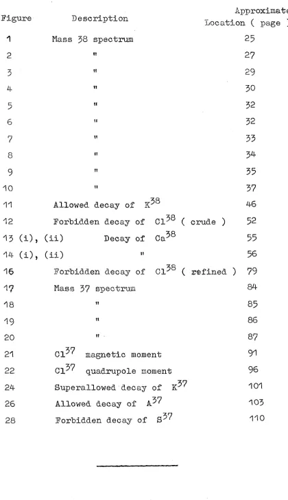
INDEX of results illustrated graphically ''^O
ACKNOWLEDGEMENTS
Introduction
{Dhis thesis describes an attempt to investigate the structure of the nuclei of mass 57 and 38. The problem, which has not been tackled in detail before, is an
int^er-esting one in that it concerns a region about" which not too much is yet known experimentally and vrhere the methods of calculation described here may begin to break down. Indeed the results obtained will indicate the applicability of an approach that has met with much success elsewhere, ( see, later, reference to the work of Elliott and Flowers ).
The nuclear problem is a many-body problem and as such cannot be solved exactly. The situation is further complicated by the fact that, unlike the atomic case, the precise nature of the inter-particle forces is not known. Hence most of the attempts to describe nuclear structure have involved the setting up of a model to represent the nucleus, deduction of properties associated with the model and comparison with experimental nuclear data.
The idea of models in theoretical physics is not new. In less sophisticated form they became the foundations of that great edifice nineteenth century ' classical physics ' thereby causing its downfall - for the conception of a
model has now undergone subtle and far-reaching development. It would be fair to say that the classical physicist did not consider himself to have understood a phenomenon until he had devised some mechanical model for its theoretical
interpretation. As most of the experiments up to that time had been concerned with phenomena which could be more or
-less satisfactorily ' explained ' along these lines, it is not difficult to understand the attitude in the 1890's that there was little else for coming generations of physicists to do than measure the next decimal place. This illusion was shattered at the turn of the century by the discovery
of radioactivity and Plancks novel derivation of the black-body radiation law, neither of which admitted interpretation via a mechanical model.
In the first decade of the present century theoretical physics was flung into confusion as one experiment after another exposed flaws in the previously well-established ideas. It is perhaps a mistake to discard a philosophy until there is something better with which to replace it', A turning point was reached however with the advent of Bohrs
atomic model and De Broglies hypothesis, the full signif-icance of neither being realised at the time. The structure of theoretical physics has now been strengthened by the
reintroduction of models, not this time mechanical, but mathematical. Thus if models are to be successful, their
limitations should be accepted and distinction made between natural phenomena and the predicted behaviour of artificial
systems.
followed by an attempt to fill in detail from nucleus to nucleus with constant reference to the measured properties. It will be seen later in this thesis just how much the work has depended on the availability of nuclear data.
The shell model
The shell model has been used exclusively as the
basis of the calculations described here. It is one of the earliest nuclear models, being the natural extension of its highly successful atomic counterpart.
The shell model has been most useful in accounting for the systematics of nuclei in a general way. It has been able to deal adequately with the structural details of
nuclei with mass lying between 6 and 20, Elsewhere detailed calculations are not always easy to perform, but generally speaking the model is not expected to give such good results.
Other nuclear models have been proposed and some have been successful where the shell model failed. However as there exists no single or unified model valid for all nuclei, the choice of a model for a particular calculation is mainly governed by the region in which the nucleus is found. In the present instance the nuclei concerned occur just before a double closed shell at Ga^^ and it was felt that in this region the individual particle shell model with intermediate coupling would prove most satisfactory as a first choice,
A description of the contents of this thesis
Chapter 1 contains an account of the Hamiltonian constructed for the calculations. The classification of nucle&r states is explained and details of the type of interaction used are
-5-given. Also included is a section on the evaluation of central force matrix elements and one on the choice of an oscillator well parameter»
Chapter 2 is concerned with the calculated energy levels for the mass 38 nuclei. It describes how the interaction
parameters were varied in order to find an ' optimum ' spectrum end discusses the final values obtained in the light of those deduced by other workers.
Chapter 5 describes the evaluation of ^ -decay log ft values from the calculated mass 38 wavefunctions» The results are used to assist verification of the interaction parameters deduced in the previous chapter.
Chapter consists of an attempt to account for the for-bidden |3 -decay of Cl^®, which could not be done using the
simple approximation to the CI wavefunction successfully employed by Goldstein and Talmi. It is shown how the CI wavefunction may be expanded using perturbation theory and how this detailed wavefunction is essential to an
under-standing of the decay. Suggestions for the resolution of this paradox are also included.
Chapter 5 considers the energy levels calculated for the mass 37 nuclei. The evaluation of magnetic and quadrupole moments in Cl^^ is also discussed.
Chapter 6 deals with the determination of /'6 -decay log ft values from the calculated mass 37 wavefunctions. A for-bidden decay, similar to that described in Chapter 4, is
Chapter 7 reviews the conclusions to be drawn concerning various aspects of the problem. Suggestions for further work on the mass 37j 38 nuclei are given together with those for possible future application of the Chapter 4- techniques.
Previous theoretical work on the mass 37, 38 problem Almost all the previous work on the mass 37, 38
problem appears to consist of passing references to one or other of the nuclei in papers dealing with systematics. A few of the more interesting references are given below.
(1) Goldhammer; Phys. Rev. 101; 1375. (1955)
This paper refers to work on 01^^, A ground state with spin is predicted followed by a low-lying excited state with s]6in /^ . A correction to the Schmidt value of the magnetic moment is suggested which is about half as large again as the experimental deviation. Mention is made of a derived quadrupole moment rather larger than the experimental one. The approach used here was to consider the coupling of nuclear orbitals through the medium of surface waves, treated by an intermediate
coupling procedure.
(2) Grayson and Nordheim: Phys. Rev. 102; 1093. (1956) This paper deals with the systematics of certain
decay transition probabilities. It shows how the ratio of theoretical ft value to observed ft value can be reduced when going from the single particle model to one using simple jj-configurations.
Allowed decay ' ' o g ^ a r '
Cl57 15 4 2.5
—> A^^ 11 4.5 1 '5
-5-(3) Kurath: Ehys. Rev, 91; 1450. (1953)
Mention is made of the ground state spin of 01^^, the value 2 being favoured. A similar conclusion is
reached by Hitchcock: Phil. Mag. 45; 585. (4) Tauber and Wu: Ehys. Rev, 95; 295. (1954)
Here an intermediate coupling calculation gives a ground state spin 0 followed by a first excited state spin 2 for Incorrect levels for are inferred but not discussed.
(5) Thieberger and Talmi: Rhys. Rev, 102; 923. (1956) Using pure jj-coupled wavefunctions the splitting
between ground and firsts excited states in A^® and some similar even-even nuclei is deduced for various forces. The level of agreement obtained in A^^ is not as good as that for the other nuclei, being only 80$ of the
experimental value.
(6) Randya and Shah: Hue. Rhys. 24; 526, (1961)
A central two-body interaction is deduced here which fits the energy levels ( of simple -configurations )
58 56
observed in , 01^ . Spin and parity are assigned to the lowest three levels in and the spectrum is
successfully related to that of 01^^, enabling the
interaction parameters to be estimated. In conclusion, however, it is shown that by this means the very small
splittings of the s^/g -particle doublets in R^^, R^^ cannot be explained.
Chapter 1
The Structure of the Hamiltonian
The basic process involved in finding the eigenvalues and eigenvectors of a quantum mechanical system is the
tt
solution of Schrodingers equation
M, ® F a; • ' ' -i- L j_
In applying this to the problem of nuclear structure H is the Hamiltonian, ^ the eigenfunctions or
wave-functioms, E the eigenvalues or energy levels of a system which acts as model for the nucleus.
The wavefunctions J may be expanded, in terms of a
complete set of orthogonal functions, such as the states formed from harmonic oscillator wavefunctions, y n
II
Schrodingers equation may then be written in matrix form, [H^ being the matrix Hamiltonian whose rows and columns are labelled by the X uy oxi« Y ^ and whose ij ^ element a.xiO- wxiuye
ii El f o)
The solution of 1.1 is then equivalent to
diagonalising [_H j . This cannot be done exactly because [ H j is an infinite matrix, but an approximate solution is found by only considering a finite number of terms in the expansion of ; ie, the lowest configuration of
The structure of the Hamiltonian depends on the details of the model used.
Classification of the nuclear states
The initial assumption made is that has doubly closed shells in neutrons and protons, from this it is supposed that low lying even-parity levels in nuclei of mass 39J 58, 57} are due to one, two, three holes in the 1d, 2s oscillator shells. It is further assumed that the classification of states is independent of whether they are formed by particles, or holes.
The next step is the enumeration of possible nuclear states formed by two or three holes in the 1d, 2s shell, such states being constructed with due regard to symmetry in the usual way. These are the 'pure' configurations in terms of which the final wavefunctions will be expressed. In the present case they have been constructed using the IB-coupling scheme for convenience, although the final wavefunctions will be intermediate between this and the
33-extreme.
For example, in mass 58 the possible configurations
p p
of two holes are d , ds and s , the IS-coupled. states
being given in the table below. The wavefunctions involve the products of charge-spin and orbital components, each with appropriate symmetry to produce a finally
anti-symmetric wavefunction.
Columns 1, 2 represent the T, S values of the two hole
T 5 L (1/3 % /O 0 1 I o b
$ 1 3
1
S ] ) 6 r M ? S
1 0 1 0
a
a.
3 31 * P F [" ] D
-These lead to the following T, J states
T
r - 0
r=
3. H-S 0 z (1^ / ? \l cls
di f
]) C:^] "]) ["1 :D
cl'' (Ax)
\z
r I
(-13 Cr
~ ' ' i i '
F [zJ -2
cT
'13
6-/ )
3,1
s TTZ? T"! ^
cC
p
s
p ["1
/
p <A ^
1-"I r
F ' 1%
Li- 31. F
eA/3 3i
b ] :D zz
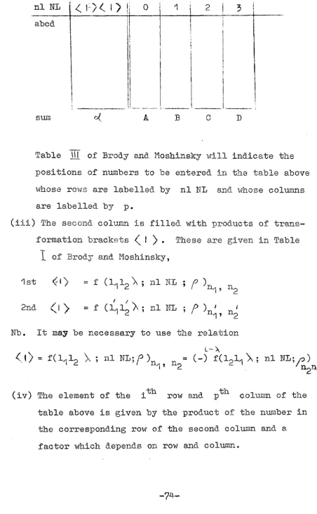
-9-These states label the rows and columns of [hJ and as J, 1 are good quantum numbers of the system, fH]j may be partitioned and the submatrices dealt with separately.
The J, T states for mass 57, which are partially classified group-theoretically, can be found in appendix
Equivalence of particle systems and hole systems It has already been mentioned that there is no difference in the classification of states formed by particles and those formed by holes.
In most nuclear structure calculations it is both easier and more convenient to work in terms of particles rather than holes. The question arises 'how may a result
derived for a system of particles be made applicable to a system of holes ?'
The type of result envisaged is obtained using the matrix elements of tensor operators. A rule given by Racah (Theory of Complex Spectra II. Phys. Rev. 52; 438» 1942) states that for a single body operator the
transition from particles to holes only involves a change of sign given by 1 + + kp + k^
( - )
where the tensor operator in question has component tensors of rank k in isotopic spin space, kg in intrinsic spin space, k^ in orbital space,
gor example matrix elements of the spin-orbit force
Racah (1942) has also shown that the matrix elements of a two-body scalar operator (eg. central force) are unaltered when holes are substituted for particles, provided only differences in energy are considered.
Terms involved in the Hamiltonian
The Hamiltonian is taken to consist of three terms: (1) a two-body central force,
(2) a spin-orbit force,
(5) a term involving the d-s single hole level separation. These terms will be discussed in more detail below. Tensor forces have not been included as there is no
conclusive justification for their inclusion in the many body problem, (Elliott and Flowers. The structure of the nuclei of mass 18 and 19. Proc. Roy. Soc. 229; 556. 1955), the spin-orbit term giving rise to similar effects.
From this it will be seen that the calculation has been carried out in Intermediate coupling, a coupling
scheme lying between the extremes of -coupling (obtained with spin-orbit force and no central force) and LS-coupling
(obtained with central force and no spin-orbit force).
[H]
The Hamiltonian matrix is given by
central force matrix 1
for holes J +
spin-orbit matri:
fof holes Vc
50 d-s difference matrix
for holes
spin-orbit matrix j y
for particles J + - ^
central force matrix for particles +
d-s difference matrix for particles
where is the strength of the spin-orbit force, Vc is the strength of the central force.
-This can be rewritten
H = ^ [spin-orbit force] + x ^central force]
jji-'S difference j| | 1 .2
1 1
—Vc
where x is the so-called intermediate coupling parameter.
The calculations were performed for several values of x . The value of ^ may be determined from the single hole
%q
levels in Ca^^ and a value of Vc chosen to give the most satisfactory agreement with experimental data. This value of Vc should not of course be inconsistent with that found by other workers.
The Central force
The central interaction between two particles outside a closed shell may be written
where r^^g is the distance between the nucleons
(X = 2s, s being the intrinsic spin of a n u d e on X = 2t, t being the isotopic spin of a nucleon
Vc
This may be expanded in terms of the permutation operators
p <r 'V
P/| 2) 2' I'/j 2 as
V^2 = W + M pfg - E + B
'I +S +T m ^ +S —.
= VCr^g) W + MC-) + E(-)^ + B(-) j v c 1^2
for two-body matrix elements, where S, T are for the
Throughout the mass 38 problem the exchange mixture
parameters ^^3 = W + M + E + B
= W + M - H - B A35 = W - M - E + B = W - M + H - B will be used.
An indication of the techniques involved in
calculating the central force matrix elements will be given later in this chapter.
The spin-orbit force.
The spin-orbit force is introduced to account for the experimentally observed splitting of certain levels.
39
Eg. In Ca^/ the 1d single hole level is split into two,
d^/E and d^/Z
Its value is „ ^
& a?.
^(s.l)>> = - for d2/2
\
= + 5/2^ for d2/2
The strength may be calculated from the mass 39 experimental levels given below (Middleton. Private
ISO
2'If 7
y communication) based on the
- reaction (He^,c4) Ca^^,
0
S It must be said at this point
/ ) %
V'GS) )( {A) that the interpretation of 3 ^ these experimental levels is
c r
by no means certain. In
particular the d /2 single hole level may well be somewhat
higher.
-15-The experimental results are difficult to analyse, furthermore Ca^^ may not "be a good closed shell. The effects of changing these levels will be considered throughout the calculations.
The value of j deduced from this data is -i-12 M e V.
The matrix elements of the spin-orbit force for mass 57 and 58 have been taken from Elliott and Flowers*
previous work on mass 18 and 19 (Private Communication).
The d-s difference.
This term arises from the interaction of particles outside closed shells with the particles inside. It is assumed to depend only on orbital angular momentum and is independent of the spin-orbit force.
The energy of particles in the unsplit d state relative to the 2s state is, from the Ca^^ data,
-2-47 + 1 68 = -0-79 M e V
Thus the d-s difference term has diagonal matrix
elements g
-0•79 in ds, ds^ -1-58 in d^, d^s -2 57 in
Calculation of central force matrix elements
An expression for the two-"body central force has already been given (equation "1.5)
Writing the charge-spin part of the two-body states as (2T + 1)(2S + 1) —
the two-body states are '
15
I— » : antisymmetric in charge-spin, requiring symmetric [2\ orbital functions for final antisymmetric state.
'11 53
I— , r — : symmetric in charge-spin, requiring anti-symmetric orbital functions for final antisymmetric state.
where the matrix elements of the j~"'s are simply the A's defined on page 15 .
Writing the appropriate orbital wavefunctions for
inequivalent particles (the symmetry of equivalent particle states being determined by the final L value) as
11.4
^ L M I Y L M )
^ u H ) ^ [^,^2 L M )" f ) )
the orbital matrix elements are
( « ' w L n i v „ i u w i n ' )
-Expanding Pjj. (cos CaJ^2^
where P (cos is a Legendre polynomial and ^ ^ 2
angle between r, and rg, gives rise to matrix elements;
-15-^Tit), L M I V I ^ ^ L M )
q° ^ I
= ^ ((,L L M I L M )
K»o
1.6
,k
where ? are radial integrals of the form of
=
) LL_ (I'J lA, ) y c{r, Ai-b 0
the 11^ being radial parts of the wavefunction normalised
by c»
1 uC Ar - (
J -n t
Prom the spherical harmonic addition theorem
(Ccr„ ) _ M r Zk+ I
V '
,Y
(0. ) (2)
the matrix elements of such operators being known. In fact
ViC&+. C + t + f')+L _ ^
[(2( + |)(2t'+l)(2l+^l)(2r4() Q L "I
( - )
2
X W Ctg't L k ) 1.7
where C are tabulated as the Shortley-Fried coefficients ((k
(Shortley and Pried. Phys. Rev. 5^; 739. 1958)
The possible values of k are restricted by the Raoah function.
The following radial integrals occur in the types of matrix element given below
1 ! 3^) P° (28^)
(d2 t 1 a2) P° d d ^ ) p2 (1d^) (Id^)
(a^i I as) (id^^ 1328)
( d ^ l I s ^ ) ( i a , 2 s )
where the have already "been defined and
=
J J
L, O
V^Cr.n) • r V' ^ J r ^ i r ,
06 O^'
"" ° 1) K y . . n ) x r U ^ . c V n
O 0
In order to evaluate the radial integrals two things must be decided,
(a) the shape of the nuclear potential well, which determines the H (r)
ix &
(b) the shape of the two-body force, which determines
V k I T l T I )
Throughout most of these calculations the nuclear potential well has been represented by an infinite
harmonic oscillator shape, following many other workers and in particular Elliott and Flowers (1955)•
V i T ) - x ( ^ . » ) "r where M is the nucleon mass
b is a constant related to the size of the nucleus whose value will be dealt with later.
This gives rise to y,
I
where the f- include a factor to normalise LL ^ as
' "A, &,
indicated above and may be found in 'The nuclear shell model' Elliott and Lane (Hand. der. Phys. 39;
2 4 1 . 1 9 5 7 )
-Concerning the two-body interaction, in the first instance a Yukawa potential
-r/a
r/a
based on simple meson field theory was chosen, following Elliott and Flowers ('1955)> with a = 1-57 x lO^^cm
Later on it was decided to vary a, the range of the force, and to facilitate this a Gaussian two-body potential
V
-r^/a^ (r) = e
was employed.
Radial intergrals with Yukawa potential.
Elliott and Flowers (private communication) have derived expressions for the d,s shell radial integrals with Yukawa potential involving the Hh functions. These are listed in appendix I, a typical example being given below
tito HKs - s i C c O H K
4- ilo HGO M j
0-5 ly
where «"<*• W " HK, W
The Hh functions are tabulated in 'Report of the British Association for the Advancement of Science' (Glasgow) 1928.
Radial integrals with Gaussian potential.
From Jahn's "Tabulation of the radial integrals by the Talmi method' (Private communication) it is seen that
^ 1/ I I ! c 1 - V v
7^^ - \
must be replaced by
(12^111 (3,. )! where /b - '
/ o 2
Three particle central force matrix elements.
So far only the simple two particle central force elements, such as occur explicitly in mass 38, have been considered.
In mass 37 the matrix elements will be given by
Using the concept of fractional parentage coefficients
(c.f.p.) to expand ^ _ 7sl
where \ \ denotes vector coupling in the T, S, L spaces and the a - are the coefficients of fractional parentage, the three particle matrix elements may be expressed in terms of the two particle ones
(Tiu)). £ , £ 1, cT
7 ' 7 it- ^
r
rUsing the fact that only operates in the coordinate space of particles 1, 2 it can be shown that
reduces to two-body terms of the form
where the integral must be unity from the normalisation
of the wavefunctions.
-19-The a - have been tabulated and are given together with the central force elements for d , d. configurations by Jahn "Theoretical studies in Nuclear Structure II'
(Proc. Roy. Soc. 205; 192. 1951)• The remaining elements have been computed from expressions used by Elliott and Flowers (Private communication).
A list of some central force matrix element expressions is given in Appendix ,11.
Evaluation of the oscillator well parameter b.
A value for b may be determined by evaluating < r > for the nucleus in two different ways and equating the results.
g
(1) For the quantum-mechanical system < r > is defined
< - > = ^ I n S
n L
where A is the mass number of the nucleus
r^ is the distance of particle i from the centre
IX (i) is the wavefunction of particle i
-n t
Thus <_>• ^ -K i U (i) Av. = J— ^ J_ 'A) F) j V' I ' A "Y"
Expressions for are taken from Elliott and Lane (1957) and the integrals I ,for nuclei with A 4 4 0 are
. 5/2 b2
I-lp - 5/2
I 2. = 7/2
I Id. = 7/2 b2
d s
exception of two holes in the d, s and so
< - ' > 3 7 - W
(2) Now is calculated using a somewhat crude technique.
Suppose the nucleus to "be represented "by a uniform spherical distribution of matter with definite radius R.
2
Then 4Lr > is given by
= - r f n = R
) i S Tcl-y xiL-kA4 ^ A
O I)
5
This approach seems no more arbitrary than that of Bwiatecki (Proc. Roy, Soc. 205; 238. 195^) who defines
b by associating R with the point at which the % r
probability density ( /b) falls to a quarter of its maximum value,
-Of course the nucleus has no definite radius, "but Moszkowski in his 'General Survey of Nuclear Models'
(Hand. der. Phys. 39; 411. 1957) quotes the following empirical formula for R
R = 1-3 X
Thus y = 1-014 A" X 10~^^cm and. equating the expressions for < r^> yields
= 1-963=x IQ-^^cm
= 1-950 X
The value of b obtained this way for the mass 19 nuclei
^19
i s b ^ Q = 1 - 6 7 2 X l O ' ^ ^ c m
- 1 ^
which compares with 1 - 64- x 10 "^cm used by Elliott and Flowers (1954).
Finally it must be remarked that it is the ratio which occurs in the evaluation of central force matrix elements, although b occurs explicitly in the expressions for forbidden /S -decay half lives and
quadrupole moments. Later in these calculations will be treated as a free parameter.
Note on the diagonalisation of CH1«
The matrix [_h] was formed by the addition of three matrices after the fashion of 1.2 for several values of the intermediate coupling parameter x .
\ji\ was subsequently diagonalised using EROS, a routine
for symmetric matrices developed by Howell (Southampton University Ph.D Thesis 1960).
Chapter 2 The Mass 38 Spectrum
The methods outlined in chapter 1 enable the energy levels with T = 0 or 1 to be calculated for the mass 38 nuclei. The available experimental data summarised in the diagram below has been taken from the following sources,
(1) Endt and Braams, Rev. Mod. Phys. 29; 685. 1957
(2) Janecke (University of Michigan), Private communication (3) Taylor (Rice University, Texas), Private communication
M e V 3-qS
5'i+-i+
3-00
> • 1 + 0
f - 7 0
O-M-S _
O - I tf o
1 T=1
.38
1-0,
-01 Ti 0
Me V
3\S!5- —
jib
O
-1
• 0
^5
A
I-I
The assignment of spin 1 to the 0«45 Me V T = 0 state in XQ
K is not absolutely certain.
The levels above 2-4 Me V are given by Taylor, those at 2' 4- and 1'7 M eV in by Taylor and Jane eke, the others being common to all three sources.
-23-The bulk of the data given on the last page, has only been recently determined. Most of the work described in this chapter was done at a time when only the lowest three levels were known in and the lowest two in Shis explains why so much attention has been paid to the lowest lying levels obtained from the calculation.
It is to be hoped that still more experiments will be performed in this region, which is a difficult one as many of the substances involved are gaseous, so that the new levels may be confirmed and spin, parity assignments made. The results of the energy level calculations will now be given and compared with the data on the last page.
Yukawa interaction (a = 1*37 % 10"^^cm)
Initially it was decided to use the interaction which Elliott and Flowers (1955) found to give such good agree-ment at the beginning of the ds shell.
An exchange mixture
A = -1
= -0*7 A^^ = +0-26
A^^ = -0'5
was chosen following that employed, in 0^^ by Elliott and Flowers (Proc, Roy. Soc. 242; 57. 1957)• The radial integrals were evaluated using a Yukawa two-body inter-action (a = 1*57 X 10~^^cm) and the oscillator nuclear potential well (b = 1*96 x ICT^^cm).
o KKJ
o
F
fr
CO
J
3r
p I
oo
V'
0
r
1 f
r •
o £ n
i>
T >»
?0
•=1
STT S
r
i
arotind 4-0 K e V, which, would correspond to x = 0*7 in this case.
The spectrum obtained is given in fig; 1 for varying values of X, These spectra have all been plotted relative to the J = 5 } T = 0 ( 3 j O ) level, which is the experimental ground state of
The following points are apparent,
(1) The first (1,0) level, which should be above the (0,1) level is much too low and falls down sharply as x increases.
(2) The (0,1) level is approximately correct, but to
gain a 2 M e V difference between this and the (2,1) level, a large value of x ('^1*2) would be needed, which is
inconsistent with (1) above.
(3) A second (1,0) and a (2,0) level, which have not yet been identified, may occur among the low lying levels in K38.
Woods-Saxon Integrals
In chapter 1 it was shown how the radial integrals depend on the nuclear potential well. One objection to the use of an oscillator potential in representing the nuclear well is that it does not approach zero as r becomes large, A better approximation to the nuclear well is the Woods-Saxon potential
V(r) = " V
1 + exp|c^(r - a)J
A
V
' Ooci f C£>. tr, cr-K
1- —> WoCtl/) - Srv
xcr-KV\ f CL/3 I.A V i /O ,-5 t J?, /)/p C"]- fc S-v V, /J T « i, cr '->.v
The radial integrals have been evaluated for a Woods-Saxon well by Wilmore (Manchester University, Private communi-cation) with = 1'16 (Ross Mark and Dawson Phys. Rev.
102; 1613. (1956)) and V = 80 M e V .
These integrals were used in the present calculation
retaining the Yukawa interaction (a = 1'37 x 10" cm). The spectrum so obtained was plotted, but is not shown here as there is no ooticeable deviation from the fig: 1 curves.
This indicates that for these energies the oscillator wavefimctions are quite adequate to describe the nuclear potential well and they have been used in all the other calculations here.
Variation of the d^/2 single hole level
It was shown in chapter 1 how the matrix elements of the spin-orbit force depended on the mass 39 single hole levels. Mention was made of the fact that these levels are not well known, there being a good chance that the d /2 level might be higher than 2 80 M e V , (which is certainly a lower limit for this level).
-o w 0"
<
i
(?
The calculation giving rise to the fig: 1 spectra was repeated, assuming that the level is at 4- M e V , the
results obtained being given in fig: 2.
At first sight the splitting between the (0,1) and. (2,1) levels has increased favourably, but the (1,0) has been pushed further below the (3,0) level. Also | has
altered (to 1 6 ) and so a given value of x now
corresponds to a larger value of Vc. As far as the lowest levels are concerned nothing can be gained from this
effect alone. However the spacing between the higher levels can be increased favourably by this change.
Initial attempts to improve the mass $8 spectrum
In this type of nuclear structure problem there are a great many quantities which can be varied. It was
decided to retain the Yukawa two-body interaction and seek improvement by variation of exchange mixture.
As a preliminary to doing this the wavefunctions for intermediate values of x were examined and found to be reasonably close to jj-coupling (see Appendix HE ).
It is not difficult to derive expressions for the slopes of the curves E(x) at the origin (x = 0 corresponding to pure jj-coupling) and from such expressions it is possible to argue whether the (1,0) curve for example can be kept
sufficiently above the (5,0), (by ensuring that its slope relative to that of the latter is as large as possible).
The slopes of the energy spectrum curves at x = 0 are
given by = - ? ( f ( w ) j j 50 | f (do) j j
x=o
-27-where He is the central force part of thevHaniiltonian
given by V^gy^Vc (see equation 1.3) and V*' (jj)j are the pure jj-couple& wavefunctions responsible for the curve with spin J,
Denoting the slope of (3,0) by
(1.0) by (0,1) by a ' (2.1) by
the following relative slopes are of interestj
Eg -E^ and E^ -E^. Using the Yukawa interaction the following expressions are obtained (in units of )
/ / /)% /t-i
Ex, -E^ = -0'49 A'^ + 0-49 A
Eg -EQ = -1'47 - 0-32 A^^
-E^ = 1*60 A^5 + 0*65 A^^ -2"06 A^^ -1*08 A^^
For an improved low level spectrum the following conditions would have to be satisfied,
(a) eJ| -E^ > 0 / /
(b) Eg -EQ > 0 and as large as possible
(c) E^ > 0
o
o
cr-vg
I
o
TT)
J
o L>
^•0
oO "P" It f\ rr
V r
& 6 fT
Jl
Exchange used by:
Elliott and Flowers Rosenfeld Kurath Soper Values
A"'5 - 1 - 1 - 1 - 1
— 0*7 - 0*6 — 0*6 — 0' 4-6
+ 0-26 + 0-35 + 0*6 - 0-15
0-5 + 1-8 + 1-0 +
0'4-Type of
exchange:-Elliott and Flowers Slope differences
E,'- E,' + 0-24
+ 0 . 9 5
E/- El - 0-76
Rosenfeld Kurath Soper
+ 1'37
+ 0 ' 7 8
+ 0*45
+ 0 * 9 8
+ 0 '69 — 0' 56
+ 0* 69
+ 0 - 7 2
- 0 - 2 3
It will be seen that none of the exchange mixtures listed here would appear to give all round improvement, with the possible exception of Rosenfelds, which is not thought to be completely satisfactory from Elliott and
Flowers (1957) 0^^ work. Also this exchange would not help the splitting between the (0,1) and (2,1) levels.
In fact two calculations were carried out using
different exchanges, the results being given in figs: 3, 4,
In the fig: 5 emrves Sogers' exchange was used. Points to be noted are
(1) The position of the first (1,0) level has improved, although it is still below the (0,1) level and is too low,
o UJ
O
(T
JO
i -O
f r
3 9 ;> b
00
\r
/» r (T
-i
f r
y
•->
I
n
T1
In the fig; 4- curves the exchange used was
= _ 1
= _ 0-7 A^^ = + 0-8 a'^'^ = 0
a modified version of that used by Elliott and Flowers, chosen to preserve — A ^ 0 - 8 from 0 .
Most of the remarks made about the fig: 3 curves also apply to this case, although (0,1) and (2,1) level
splitting is a little better.
From these results it was concluded that variation of exchange mixture alone could not improve the mass 38
spectrum. This was born out by the f?> -decay results to be discussed in chapter 3«
Attempt to simulate a variation in the range of the two—body force.
/ t
The expressions derived for etc. above depend on the exchange mixture and the two-body interaction. As variation of the former yielded no improvement, it was decided to vary the latter.
An attempt to simulate the effect of varying the range a of the two-body force was made by introducing a quadrupole force of strength ^ defined by
V (r) = 'Zl_, r? r^ Pp (cos ^ ij)
i < j 1 J ^
There is little justification for this new force. Its physical interpretation is vague; all that can be said is that it resembles the interaction between two particles outside a closed shell and the vibrations of the closed shell core.
New expressions for etc, were worked out, various exchanges considered, and a rough estimate of the value of
^ made. Detailed calculations were then performed following the usual techniques.
It has not been thought worthwhile to include a
summary of the results obtained, some of which seem rather peculiar. The quadrupole force did help to increase the splitting between the (0,1) and (2,1) levels but this was completely offset by a considerable deterioration in the position of the lowest (1,0) level.
This approach was then abandoned in favour of a straight-forward range variation.
Variation of the range of the two-body force
The effects of changing the two-body interaction are felt in the evaluation of the radial integrals. It was decided that as the range might have to be changed several times, this would become easier if the Yukawa potential were replaced by its Gaussian equivalent. This had the additional advantage of demonstrating the effects of changing the shape of the two-body potential.
It was shown in chapter 1 how this step was carried out.
-15 Gauss potential, a = 1"80 x 10 cm.
This short range potential is similar to the initial
-51-o
N
--T
0^
00
i
O3 (TT
-2 i>
oo
IQ
f\
rr
t
£ m 6
rr
<r-<
31. T
Yukawa calculation with a = 1•57 x The Elliott and Flowers exchange was again used.
The spectra obtained are illustrated in fig: 5* It will be seen that there is little or no improvement.
("1) The first (1,0) level is much too low and again falls shatply as x increases.
(2) The (0,1) level is much too high and consequently cannot easily be split 2 M e V from the (2,1) level. (3) A second (1,0) and a (2,0) level should be found in
the low lying levels of
The range of the potential was then lengthened.
Gauss potential, a = $"40 x 10"^^cm.
This calculation was first performed for the Elliott and Flowers exchange, the results obtained appearing in fig: 5.
Significant changes have occurred, but no improvement. (1) The first (1,0) level is now a little higher,
(2) The (0,1) level is ridiculously high and cannot besplib
2 M eVfrom the (2,1) level. (3) The second (1,0) and (2,0) levels are again low.
Having observed the effect of a range variation it was decided to see whether altering the exchange could cause an improvement. Expressions were worked out for the slopes of the curves at x = o as indicated before.
-E^ = -2'8i
Eg -E^ = -2-7'
o
A-'5 + 2-84 A-T)
- 0-45 A53
o
<r^
co
I
o o fN> 6
From these it becomes clear that one way of reducing the slope of the (0,1) curve was to change the sign of This also slightly assists with the splitting between the
(0,1) and (2,1) levels. Changing the sign of also helps. From other considerations it is not advisable to alter ^ or A^^ and so it was decided to try the exchange
A-"? = — 1
A5^ = — 0 • 7
A35 = — 0'26
A''-' = + 0*5
which is similar to that favoured by Soper (and will here-after be referred to as the Soper-like exchange).
The curve slope data is summarised below
Exchange;- Elliott and Flowers Soper-like Values
—E^ + 1'42 + ^1-* 26
+ 1-80 + 2-03
'2 ^o
-®o'
Ej'-E/ - 6-97 + 1-05
The calculation was repeated using the new exchange and the result obtained is illustrated in fig: ?•
(1) The position of the first (1,0) level has improved and is now roughly correct for 0 1 < x < 0-5
(2) The (0,1) level is still much too high and the split-ting between this level and the (2,1) has only
improved slightly.
r\
NJ
f
cr>
00
o
JT <?
It is known that reducing the range of the force improves the position of the (0,1) level. It was decided to try a mid range potential to see whether the (0,1) level could be lowered and the lowest (1,0) level kept sufficiently high.
Gauss potential, a = 2 $1 x 10~^^cm.
The calculation was performed using the Soper-like exchange, the results being given in fig: 8. These were the best obtained for the low lying levels in mass 38, the wavefunctions associated with them also being the most satisfactory as will be seen in the next chapter,
(1) The position of the first (1,0) level is still improved but it is still too low for a realistic value of x, (2) The (0,1) level is again too high (but at least for
x < 0 ' 3 it is above the (1,0) level for the first time). If this level could be further lowered and the (2,1) raised, the splitting between them would be correct. (3) The second (1,0) and (2,0) levels should be low lying
in
The -decay calculations in chapter 3 indicated that a value of X around 0-5 should be taken, corresponding to
38
Yc 'V 30 M e V« The spectrum so obtained is compared
with experimental data below.
+
n<v 1 T- I
18 — r - — — , _
1-7 — %+ T.o / — r^o
O-Q O^T^-L,
, 4. ,0-u-s c
•A I T_ 0' ""O IU /-)+ \
The arrival of new experimental data caused attention to be turned towards some of the higher levels.
The evidence was strongly in favour of there being only one level between = 0 at 0-45 M e V and 2"^T = 1 at 2- 4 MeV, whereas all the calculations so far have advocated two (for realistic values of x ).
The position of higher levels in this kind of treat-ment must depend quite strongly on the single hole levels which represent the pure jj-coupled states at x = o.
It was said earlier that the d^/2 single hole level at 2-80 Me V could only be taken as a lower limit. If this level were to be raised, it should lead to the raising of the higher calculated levels leaving the lower ones relatively unchanged.
The calculations were repeated using the Gauss mid range force, the Soper-like exchange, and a d^/2 single hole level
shifted from 2-80 to 4 Me V. The results for the lowest levels are shown in fig: 9.
(1) The position of the first (1,0) level is acceptable for 0-1 <- X < 0- 4.
(2) The (0,1) level is again too high and is only below the (1,0) for x<.0 2. In order to obtain good splitting between the (0,1) and (2,1) levels a high value of x
('^ 0 7) would be necessary, at which both of these levels are too high by 1 M e V .
(5) If there is to be only one level between the (1^)T = 0 and the 2^T = 1 then 0 - 54 < x <1 0 • 42 .
Taking all these factors into account together with the /3 -decay data of chapter 3, the best overall agreement is
-55-still obtained with. Vc = 30 M e V which now corresponds to X = 0-58 (since ^ has changed to —i-S M e V).
The spectrum with Vc = 30 M e V is compared with the experimental data below for the lowest levels.
f T.c
T=0
r,v
asc
'lU-O
' 10
2*7= I
T-o
0-7
ozs 0
C(^lc\xXat & d
1 = 0 1=0
- O'l+s
o
4-Q 3"T=0
tx|. 411 g ',-L b A
The following remarks can be made,
(1) The T = 0 level observed at 1-70 M e V is probably the 1"^ T = 0 calculated to be at 1-5 M e V.
(2) The next even parity level above 2'^T = 1 at 2-40 Me V is most likely to have spin 2 with T = 0.
The spectrum with Vc = 30 M e V is compared with the experimental data below.
415
tf 2 c
315
+
tf"" • t
2 T. !
•I
y
t
The lowest calculated 2'^T = 1 level is out by 1 M e V and further comment is impossible until more experimental data is available.
Fig; "10 illustrates the complete level scheme obtained from this last calculation.
The final conclusions to be drawn from these results will be left until chapter 7*
Justification of the longer range force
The mid range Gauss force used here has longer range than the conventional p shell forces and indeed longer range than that required by Elliott and Flowers (1955) at the beginning of the ds shell.
Some workers at the beginning of the pf shell have also found it necessary to employ these longer range forces.
The assumption of a long range force was first made by Kurath (Phys. Rev. 80; 98. 1950). Levinson and Ford
(Phys. Rev. 100; 13. 1955) had to employ such a force
iLp
when fitting a spectrum to Ca . French and Raz (Phys. Rev. 10^1-; 1411 . 1956) also used a longer range force
(though not as long as Levinson and Ford's) when investigating the spectra of Ca isotopes.
If all these results are valid, there is no reason why a force of longer range should not be required just below Ca^*^.
Analysing the results quoted in French and Raz ( 1 9 5 6 )
( 1 ) Levinson and Ford used a very long range Gaussian
Potential and Range Nucleus ^/K ^/Vc Vc (M e V )
Yukawa a = 1•37 x Li^ 6 21 0 031 32 5 62 0 024 42
Gauss a = 1-80 X 10"^^cm Li^ 8 47 0 023 44
M 6 78 0 022 45
Gauss a = 3 40 x lO^^^cm 4 0 o - o i l 93 28 1 0 013 68
Gauss a = 2-51 X 10~^^cin Li^ 14'7 0 020 49 10 5 0 022 43
-38-(2) French and Raz used a Gaussian force of range
a = 2 7 X 10"'^ ^cm. To fit the Ga^^ spectrum they
required an overall Vc 'v 25 M eV. (Nb it proved easier to fit the spectrum than the Ca^^).
They also used an exchange mixture having
= 2 5
which is similar to the value 2-? used here.
Using a Gaussian force of range a = 2 31 x 10"^^cm and overall Yc 30 M eV would not be inconsistent with the above.
Some calculations were made to investigate the effects these longer range forces would have had in the p shell.
The quantities ^/K and ^/Vc were evaluated.
Kurath (Intermediate coupling in the 1p shell. Phys. Rev. 101; 216. 1956) found empirically that ^/K should lie between 6 and 7 whilst K 1 M e V.
The results obtained are summarised in the table opposite. Vc was estimated by putting K = 1 Me V.
Chapter 3
The Mass 38 Wavefunctions
When the Hamiltonian matrix [n] described in chapter 1 is diagonalised, a set of eigenfunctions are obtained which
If
are the approximate solutions of Schrodingers equation. These functions represent the nuclear wavefunction and may be used to calculate such things as transition probability for electromagnetic radiations, /'S -decay ft values, magnetic and quadrupole moments.
The mass 38 wavefunctions have been tested via the calculation of several -decay ft values. The available experimental data, taken from Endt and Braams (1957) is summarised in the diagram below.
HeV
1,9 A (T
•) 4- o . J - " +
-c + O •
K 58
I f O
" '- t s j
A
In addition to this there is the decay which will be considered later.
The composition of some mass 38 wavefunctions is described in Appendix III
The allowed -decay transitions
In light nuclei most /3 -decay transitions are of the
allowed type for which the ft value is given by (Elliott and Lane (1957))
ft = 1 ; 3.1
(1-x) 1 + X G
where the square of the Fermi matrix element is %
/ . IXM) ± '",'«) \ f ) 5.2
and the Gamon-Teller term
2,
(+' 1"''J 5^3
the 'dashed' symbols representing final states and the ±.
±
signs referring to yS emission
B and x are constants given by
B = 2785 it 70 X = 0'560 ± 0-012
The Fermi term
Rewriting the Fermi term operator in terms of TV, where
Hr
-are defined such that "Y is the operator which changes a proton into a neutron and is the operator which changes a neutron into a proton, and using the
Wigner-Eckart theorem, it can easily be shown that
where T is the nuclear isotopic spin and M - the 1%^ value for the final nucleus. It will be seen that this term cannot contribute if isotopic spin
changes.
For example consider the super allowed decay
(0+^ T=1; M =0) (0+, T=1;
then = ( 1 + 1 ) ( 1 - 1 + 1 ) = 2
The G-amow-Teller term does not contribute in this case because the vector operator concerned cannot couple two J = 0 states.
Thus from 3.1
ft = — ^ 2 8 3 whence log.^ ft = 5'5
(1-0-56) 2 'U
This example gives no fresh information because the decay concerned was used in establishing the constants of the
ft formula.
The Gamow-Teller term
Writing the operator in terms of ,
1 (fV'rVTn;)l£Y.,(»<r>jf (TM^J M,))
Applying the Wigner-Eckart theorem to remove M dependence
I \ 1 <
(.2 ^ ^ L _ . . . V. -^ r27'+,)(Z3'-^l)-^T,-^rttV j
I \
C
4'
Z \
-42-r n
where ^ a r e the Wigner coefficients.
This is an amplitud.e matrix in both T and J spaces.
Using the latent symmetries of the Wigner coefficients and their orthogonalities it is not difficult to show
c"' )"
/ 2J + 1
Hence ^ . u , , >
>
where , t ' m ' ^
c ' (2T'+1)(2J+1) My
Consider
N = (^f'(TV(t7')U'jn'!!£T;<l)'^w||f(Ti(««[+]n)j
where (1 1) [ f1 L denotes a two-body orbital angular
momentum state where 1, 1 of the two particles have been coupled to form a state of symmetry [fl .
As the operator in N does not operate in the L space but only in the T, S spaces
N
X f r ' b l
^ ^ 1^6
using standard expressions of the Racah algebra, to be found for^example in Elliott and Lane (1957)•
For antisymmetric two particle states
( T V . a(T's'hu><rfe>||Ts)
= l ( r ' K w l i T ) ( 5 ' K w i i s
since Y only operates in the T space and tr in the S space.
These terms may be evaluated using the fact that the operator does not act on the first particle
( t ' N w | |T ) = ! {IT'+ i )(3T+1)] TV, I' ^ T ' ) I!
and similarly for the other. Also
(Hii'-iiH) -- *|T
Hence >2
N . ^ L,(<
l)['"
.+T.L+r+s.'+i (L-3 S
1
SI5 I
^ | i s ' 7 ' ) ( i T ' j l l - i S ' j
5.7
11
In solving Schrodingers equation the nuclear wave-functions were expanded in terms of certain LS-coupled.
states
4
Hence from 5'5 1. A
2L %
A ( i k % I (9 li £ 4-;
y / i
(
where (0 represents the appropriate operator, and
' ' ,
( % (0 II Yi ) is oust N evaluated "between states which are known.
?
The evaluation of G from 5.8 is equivalent to forming the matrix representation of with rows labelled by the
^ and columns by the , pre- and post-multiplying by the appropriate eigenvectors obtained from the calculation, squaring the result and multiplying by A.
ie. = [<r, ' - ]
U ' (9
t
+
The allowed decay ,
The details of the decay are
(5+, T = 0)
Z . a58
a ,a .
x A
(2+, T = 1)
3.9
The matrix [ (9 ] is labelled by the states (J = 2 , 1 = 1 ) and (J = 3, T = 0) as in the diagram.
The zeros are caused by A'
<r./)
l<"
d />15
J)
13
G-t
It .1
p o 0
P o 0 o
o
11
F
o o31
1)
DC
ID
o
c
Fife.. 11 Lc*:, -f-t
15. ?c h g 1- (. t cv
Vfv 1 u e 5
'Z M- - la . <? 1 o
is determined from the relation
= < ®j,> = i (N - Z )
3.10
for a nucleus with N neutrons and Z protons. Eg. for which has N = Z = 19; M ^ = 0
for which has N = 20,Z = 18; M = 1 $
In this example A, evaluated from 3.5i has the value /42.
Thus G can be found when the calculated eigenvectors are substituted in 5*9 and log^Q ft obtained from 5.1 where the Fermi term does not contribute, there being a change of isotopic spin.
The matrix elements of [Q] were checked by calculating this fi -decay using pure jj-coupled wavefunctions directly, which corresponds of course to x = 0 in the eigenvector calculation.
The results obtained are given for several exchanges and ranges in Fig: 11; a key to these curves is given below.
Exchange Curve no 1 2 5 4 5 6 7 8 9 a5/2 Potential
<XX (0 <.T>v
Yukawa i'37 2-8 MeV "
4-" 2 8
Gauss L go S 40
1
3 A 5 3
-1 - 0 - 7 +0 -26 -0-5
tt n tl It
tt — 0 ' 4 - 6 -0-15 +0-4 11 - 0 ' 7 +0 8 0
11 n +0 26 -0-5
ii 11 11 11
ti It -0-26
+ 0 - 5
n 11 t l tl
The experimental value for log^Q ft is 5-0. The
results will be discussed on. the basis that the calculated ft is acceptable if it lies between 4-- 8 and 5'2. (a) Curves 1 to
These curves were obtained using short range potentials and various exchange mixtures. One variation of 6^/2 single hole level is included. For an acceptable log^Q ft X must be restricted as follows
Curves 1 , 2 x > 0-9 Curves 4, 5 x > 0 8
Reference to the spectra associated with these curves (Chapter 2) shows that with these values of x no
kind of agreement can be obtained with the experimental levels, due mainly to the positions of the two lowest (1, 0) levels.
(b) Curves 6 and 7»
These curves correspond to the long range Gauss potential, with a variation of exchange. For an acceptable log^Q ft x is restricted as follows
Curve s 6 0 24 <L x < 0 - 4 2 Curves 7 0-14 < x < 0 - 3
Reference to the spectra associated with these curves (Chapter 2) shows that if x is so chosen, the spectra will not agree with experiment due mainly to the
position of levels (0, 1) and (2, 1) in addition to the totally inadequate splitting between them.
(c) Curves 8 and 9*
These curves represent the Gauss mid range force with a change of d^yg single hole level. It will be
-4-7-observed that this ealculation is particularly insensitive to the latter effect. For an acceptable log^Q ft x would be restricted by
0 52.C % C O 6
Reference to the appropriate calculated spectra (Chapter 2) shows that x lying within this range will produce a spectrum that may reasonably be compared with
experiment.
In particular Vc = 30 M e V which gave the best spectrum corresponds to x = 0-5 in curve 8 and x = 0 $8 in curve 9? both of which lie within the range above.
The very faint indication that increasing the d5^2 single hole level leads to a decreased value of x for the same level of agreement with experimental (% -decay data should be noted; this result would seem to apply with regard to energy levels (Chapter 2).
Conclusions to be drawn are
(i) the calculation is sensitive to range of potential and exchange, it being necessary to employ the longer range to obtain agreement with experiment for -decay and energy levels,
(ii) this calculation is insensitive to the <3.5^2 single hole level position.
The forbidden -decay Cl^^
The ^ -decay (0*) is of the unique
Expressions may be derived for the f^t value of such a decay, one of which is given below (see Blatt and
Weisskopf 'Theoretical Nuclear Physics' or Bohr and Mottelson Dan. Mat. lys. Medd. 27; 16. 1953)
f.t
• z j r V x
I\B)
(Z,E„)
M
1^)
I IV, ' ' 5.11
where x, B were given at the beginning of the chapter Z is the number of protons in the nucleus E^ is
p the total energy available for the decay (units mc )
fl.} Ifoi L
is given by
Davidson (Phys. Rev, 82; 50• 1951) who also plots a(z), b(z) as functions of Z.
Now
< I (T'M; 11 Mr J n , )
C 1 ' I »
t1(n-can be reduced using the Wigner-Eckart theorem and the orthogonality of Wigner coefficients to
•y
t / /.-/ ^ y i / t .
- ( T ' m ; J ' 11 t - ^ K x A - \ r ) I T n j )
2 J 4 I \ ' "I
an amplitude matrix in the J space. This expression can be evaluated using suitable wavefunctions.
The technique followed here will be to substitute crude wavefunctions for Cl^®, on both sides of 5»'^2 and add detail later.
The lowest energy odd parity configuration of CI (J = 2) is
I K f (hx)' J
(hvj ['»%)
(i-r </ fc-ffix
which would appear from the work of Goldstein and Talmi (Phys. Rev. 102; 589. 1956) to be a good approximation to the real wavefunction.
If this is to decay as a first forbidden transition to ^38 (0"*"), the only part of the argon ground state wave-function that can contribute is
) 'k. C u-t TO -r
Z ") I", r <T t.c VL. j
Thus the nuclear states may be represented by the following simple wavefunctions in jj-coupling
01^^ = u; )( (.) Yf:; - X,w c(3, (V X (') i ^ 7'%
Y Xy"
L * " ^ ^7^0
where ^ represent wavefunctions for neutron, proton.
Defining
N = (/A
j f
where y ( 1 2 ) , ^ (tz) are just as given above, and using
the properties of T_ : t ^ = 2 X - = °
reduces this to
Since the operator only acts in the space of particle 1,
N - k (''•h h " It ( h )
ViOC \ /
3C
2 •v
< = ;
from further properties of the operator. Evaluating this expression
( i II i ) = \f6
,2 m y1„ ,3^ _ _ ± /lis" IT (Y 0 r H r?) = - ?
oO
J U,_ u. rJ^r b 0
f—
whence N = f7 h, where "b is the oscillator well V TT
parameter.
The value of 5-12 is therefore 7 5 T
For this decay = 4-9 M e V (Endt and Braams (1957) ) = 9 68 (mc^)
for Z = 18 a(z) = 0 0 5 2 1
r Davidson (1957) -b(z) = 0-054 J
and b = 1-963 x ICT^^cm (Chapter 1) = 5'105 X 10"^ cm C^-^/mc )
Substituting these numbers into equation 5.11 yields
losio fot = 6 77
%8
The detailed A wavefunction
2 The log ft above was evaluated using a (<3-5/2
58 configuration for the ground state of A .
The J 3 0, T = 1 ground state wavefunction calculated for consists of a linear combination of jj-coupled states
f' (a58) = (a 5/^ )2 + /3 (a 3^ )2 + % (Sy^)2 3 ^
where c( ^ + yS ^ + y = 1
-51-— VI (/)
~~r
1 ?
% 5
(T
5>
<-& f
I
5
*>
/r # O
IT
A
V
5-«
r >
P
! (A ,
\> '
Z)
Jl (?
Since only the (d^yg)^ configuration contributes to the decay it will be necessary to include a factor ((3 is a function of x ) in $#13, the initial expression for W carrying this factor through, the final expression
becomes
" 2 (x) 3,15
The values of/3 (x) are determined by transforming the 16-coupled wavefunctions into their jj-coupled equivalent.
Pig: 12 illustrates the results obtained for several ranges and exchanges; the curve numbering here is as in Pig: 11.
It will be seen that none of these curves predict the experimental figure. This result is disappointing in view of the previous success of the Gauss mid range force
(curves 8 and 9).
One reason for this non-agreement might be that too crude
3 8
an approximation has been made in the 01 wavefunctions. It was decided to repeat the calculation using perturb-ation theory to form more realistic wavefunctions by the mixing in of higher configurations. The next chapter (4) will be devoted to this approach and the conclusions to be drawn therefrom.
Another possibility to account for the bad agreement is that the oscillator well approximation to the nuclear potential is too crude. It seemed hardly worthwhile to replace this by the Woods-Saxon well, which in chapter 2 led to no significant change in the energy levels.
-52-However the more drastic change of substituting an infinite square well potential was investigated.
The effect of this is to replace 'S = J ^ h ±n the original calculation by
N 2 - 9 5 6 0 11
V 2
R
where R is the 'nuclear radius' obtained from the empirical formula quoted in Chapter 1.
Expression 3-15 is thus replaced by
lo&IO = G'98 - 2 (%) zg
and even including the expansion of the A ground state it would not be possible to obtain good agreement with the experimental result.
/3 —decay of Ca^^
Cline and Chagnon (Phys. Rev. 108; ^957) have
reported the decay of an unstable calcium isotope formed from the reaction
Ca 4-0 ( % , 2n ) Ca 38
The experimental data for this decay is given in the diagram below.
On the basis of the shell model Ca^® is a T = 1 nucleus which should have a
Two 11^ decays were observed consistent with log^Q ft = 5-5. One of these was associated with the superailov/ed
transition . «+
Ca58 (o+, K58 (o+, 1)
The other apparently gave rise to a - ray of energy 3-5 Me V, and was interpreted as a decay from the Ca^® ground state to a 1+, T = 0 level at 3-5 Me V in
A theoretical investigation was made as to whether this interpretation is consistent with energy levels and wavefunctions obtained in the present calculation.
An alternative interpretation of the second decay, suggested by Cline and Chagnon (1957) was
Ca^G (o+, (o+, 1) at 3-5 Me V,
which would be inconsistent with these calculations as they do not predict a (0^, 1) level for in this region,
A theoretical point also arises here. If there were no Coulomb force the decay would go exclusively via the transition to the lowest (0*, 1) level in The existence of a Coulomb force will admittedly mix the
(0*, 1) states, but hardly to such an extent as to account for the second decay observed by Cline and Chagnon.
38
It was decided to treat the Ca ground state as
(0*, 1) and calculate the log ft values for ^decay to all the predicted (1"^, 0) levels.
The theory of such allowed transitions has already been, described earlier in the chapter. The decay under
consideration involves a change of isotopic spin, so only the Gamow-Teller term can contribute.
-54-N cr < 4 Z m
in
31
N>