A Comparative Study on Analysis of Various Shortest Path Algorithms on GPU using OPENCL

(1)

International Journal of Computer Applications (0975 – 8887) Volume 179 – No.40, May 2018

34

A Comparative Study on Analysis of Various Shortest

Path Algorithms on GPU using OPENCL

Umesh Nayak

UIT, RGPV Bhopal

Rajeev Pandey

PhD, Asst. Professor

UIT, RGPV Bhopal

Uday Chourasia

Asst. Professor

UIT, RGPV Bhopal

ABSTRACT

Finding shortest path for various applications is important in various domains. But to provide result for complex graphs in real time is a challenging task. So in this paper four shortest path algorithms namely Dijkstra‟s algorithm, Floyd Warshall, Bellman Ford and Jhonsons algorithm are studied and analyzed to detect parallelism in them and the parallelized version of all three is implemented using parallel computing framework OpenCL. It is found that Bellman Ford and Floyd Warshall contains fine grained parallelism while Jhonsons has less parallelism.

Keywords

Bellman-Ford, Dijkstra, Floyd Warshall

1. INTRODUCTION

In this world of quickest growing technology, computers have become a lot of powerful than ever before. thus it‟s a difficult task to create economical utilization of all the resources inside a machine. In period of time solely central processor area unit concerned in programming however currently each day GPU that area unit termed as General Purpose Graphical process Unit (GPGPU) also are on the market in concert of the resource which may be equally utilised and might offer high performance at an affordable value. GPU area unit like minded for applications that involve the utilization of matrices thanks to its design.

One of the applications is shortest path issues on graph that deals with matrices.

Shortest path [1][4] drawback finds application in massive domains of scientific and world. Common applications of those algorithms area unit in network routing, VLSI style, artificial intelligence and transportation, they're additionally used for directions between physical locations like in Google maps. Here all the applications mentioned usually involve positive weights however some applications area unit there wherever weights will be negative like currency exchange arbitrage and a few alternative areas wherever, edge represents one thing aside from just distance between 2 entities. In such application areas Bellman-Ford algorithmic rule will be used. Bellman-Ford algorithmic rule is applicable on graphs with negative weights and might additionally notice negative cycles wherever majority of algorithms fail. tender-Ford is additionally utilized in wireless detector networks and alternative impromptu networks as distributed Bellman Ford will be used there. Distributed Bellman-Ford is additionally used as initial ARPANET routing algorithmic rule [12] in 1969 .

Most of the higher than application area unitas specified are real time applications and wish leads to a fast time that the performance of algorithmic rule have to be compelled to be improved so it consume less power and time.[8] Parallel computing on GPU is one in all the technologies that area unit

used for top performance computing at an affordable value and considerable speed of performance. GPU is presently used for a range of functions with the exception of graphical process and play. That‟s why we tend to refer GPU as General Purpose Graphical process unit (GPGPU) because it provides high performance computing will be programmed victimisation commonplace frame work like OpenCL and CUDA. OpenCL could be a framework that is for all GPU whereas, CUDA is supposed specifically for NVIDIA GPUs solely. Thus, we are going to be victimisation OpenCL for our GPU implementation thanks to its movableness and open-ness

2. INTRODUCTION TO OPENCL

Open Computing Language may be a framework for writing programs that execute across heterogeneous platforms. They consist as an example of CPUs GPUs DSPs and FPGAs.

[image:1.595.326.534.447.536.2]

OpenCL [11] specifies a programing language (based on C99) for programming these devices and application programming interfaces (APIs) to manage the platform and execute programs on the figure devices. OpenCL provides a customary interface for parallel computing mistreatment task-based and empiric similarity.

Figure 1. Actors on OpenCL system

Heterogeneous systems

It's a system composed of multiple computing systems. as an example a desktop system with a Multicore processor and GPU. Here area unit the most elements of the system:

Figure 2: OpenCL Platform Model

[image:1.595.334.522.616.703.2]

(2)

35 You don't need to think too much on how the OpenCL device

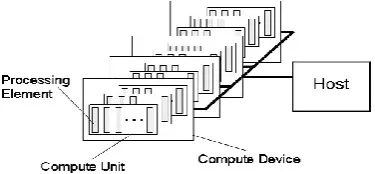
[image:2.595.58.275.117.281.2]

model fit on a specific hardware, this is the responsibility of the hardware vendor. Don't think that Processing Element is a "Processor" or CPU Core.

Figure 3: AMD GPU Compute Device

OpenCL Models

First to understand OpenCL we need to understand the following models.



Device Model: How the device look inside.



Execution Model: How work get done on devices.



Memory Model: How devices and host see data.



Host API: How the host control the devices.

OpenCL components

 C Host API: C API used to control the devices. (Ex: Memory transfer, kernel compilation)

 OpenCL C: Used on the device (Kernel Language)

[image:2.595.318.551.222.534.2]

Device Model

Figure 4. Device Model



Global Memory: Shared with all Device, but slow. And is persistent between kernel calls.



Constant Memory: Faster than global memory, use

it for filter parameters



Local Memory: Private to each compute unit, and shared to all processing elements.



Private Memory: Faster but local to each

processing element.

3. INTRODUCTION TO GPU

ARCHITECTURE

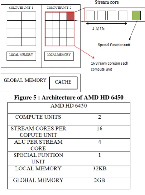
To make efficient utilization of resources one need to be fully acquaint with architecture of those resources especially like GPU[9][10]. GPU comprises of one or more compute units and compute units further consists of stream core processors. Each stream core processor consists of some ALU‟s and special function unit. In VLIW5 architecture it consists of 4 ALUs and 1 special function unit. All the stream core processors within a compute unit share local memory and global memory is shared by all the compute units. The architecture of GPU on which implementations are tested i.e. AMD HD 6450 is shown in figure 5.

Figure 5 : Architecture of AMD HD 6450

Table 1: Configuration of AMD HD 6450

4. RELATED WORK

[image:2.595.57.280.299.710.2]

(3)

36 Bellman-Ford implementation, achieving rates up to 14x

higher on low-degree graphs and 340x higher on scalefree graphs. we have a tendency to additionally see vital speedups (20–60x) compared against a serial implementation on graphs with adequately high degree.

In [2], they describe a variant of the Bellman–Ford algorithmic rule for single-source shortest methods in graphs with negative edges however no negative cycles that willy-nilly permutes the vertices and uses this randomised order to method the vertices among every pass of the algorithmic rule. The modification reduces the worst-case expected variety of relaxation steps of the algorithmic rule, compared to the previously-best variant by Yen (1970), by an element of 2/3 with high likelihood. we have a tendency to additionally use our high likelihood certain to add negative cycle detection to the randomised algorithmic rule.

5. BELLMAN FORD

Consider a graph G(n,E,V) where, n is that the range of vertices, E is that the set of edges and V is that the set of vertices. contiguity matrix illustration of graph is employed here, because it is like minded for GPU.[3][5] Here, price is that the contiguity matrix for graph. Initially, Dist can contain direct edges from the source„s‟. Afterwards, Dist[v] of „kth‟ iteration means that distance from „s‟ to „v‟ browsing no over „k‟ intermediate edges. Finally, once no-hit completion of rule Dist can contain the shortest path to any or all the vertices „v‟ in V from source„s‟. for every edge (u,v) in set E, Relax(u,v) is termed (n-1) times. So, Relax () is termed E (n-1) times, therefore majority of your time of the rule is spent during this procedure. The rule for Bellman Ford[6] is illustrated in rule 3.1.

BellmanFord (s,Dist,Cost,n)

{

for i=1 to n do

Dest[i] = Cost[source,i];

End for

for k=1 to n-1 do

for each (u,v) in E do

Relax(u,v)

End for

End for }

Relax (u,v)

{

if Dest[v]> Dest[u] + Cost[u,v]

Dest[v] = Dest[u] + Cost[u,v]

}

Time complexity of Bellman ford algorithm if adjacency matrix representation is used will be O(n3) .

All pair shortest path using bellman ford algorithm could also be calculated if above algorithm for all the vertices in the graph is called.

For each s in V

Call BellmanFord(source,Dest,Cost,n);

End for

Identified Parallelism:

The only issue arises here is the way to calculate minimum of of these „n‟ values. therefore instead of conniving the

minimum which is able to increase the time of algorithmic rule we'll synchronize the write operations on Destk[v] for all „u‟ specified minimum worth resides in Destk[v] at the and of Relax() procedure. This issue is referred as write-write consistency.

6. FLOYD WARSHALL

APSP may be a elementary drawback in graph theory. Floyd-Warshall (FW) may be a accepted algorithmic rule for its resolution. FW sequent implementation uses 3 nested loops.

Consider a weighted graph G (V, E) hold on mistreatment nearness matrix illustration by a weight matrix W of order N*N wherever N is variety of vertices in G.where, wijϵ W for all (i,j) ϵ E.

This matrix W contains zero for diagonal components as each corresponds to same vetex. And eternity for the vertices that aren't connected directly and weight is there for vertices that area unit connected directly or edges out there in graph.

Floyd algorithm:

For(int k=0;k<N;k++)

For (int i=0;i<N;i++)

For(int j=0;j<N;j++)

Identified parallelism:

As it is evident from the on top of algorithmic program that price of kth iteration depends on k-1 therefore this loop contains dependency therefore it can not be removed to perform correspondence. however rest two loops will be referred to as in parallel for N2 threads victimization OpenCL.

7. DIJKSTRA’S ALGORITHM

Dijkstra algorithm[7] ia a single source shortest path algorithm and it can only be applied to connected graphs having positive edge weights.

The Algorithm consists of following steps :

•

Distance to supply vertex is ready to zero. • Set all different distances to eternity.

• S is ready of visited vertices that is empty at first. • Q is that the queue that at first contains all the vertices.

• Then till letter of the alphabet is empty part is chosen from letter of the alphabet with minimum distance. • And then this u is added to visited vertex list. • If new shortest path found is shortest among all it's set as new shortest path until this step

Dist[S]  0

For all v ϵ V – {S}

Do dist[v]  ∞

S  ᵠ

Q V

While Q ≠ ᵠ

Do u  min(Q,dist)

S  S U {u}

(4)

37

Identified parallelism :

For all the vertices in Q we are able to execute below steps in parallel and notice the vertex victimisation write-write

consistency that holds minimum distance price. in order that the gap came are going to be the smallest amount of all the

vertices processed in parallel.

8. JHONSONS ALGORITHM

Johnson's algorithmic rule could be a thanks to realize the shortest ways between all pairs of vertices in an exceedingly thin, edge weighted, directed graph. It permits a number of the sting weights to be negative numbers, however no

negative-weight cycles might exist. It works by mistreatment the Bellman–Ford algorithmic rule to reckon a metamorphosis of the input graph that removes all negative weights, permitting Dijkstra's algorithmic rule to be used on the remodeled graph.

Comparative Analysis

ALGORITHM TYPE COMPLEXITY GRAPH PARALLELISM

Dijkstra SSSP and APSP O(n2) and O(n3) Positive edge weights only Coarse grained parallelism

Bellman Ford SSSP and APSP O(n3) and O(n4)  Negative and positive both.

 Can detect negative cycle also.

 But doesn‟t works for graph which contains negative cycle.

Fine grained

parallelism

Floyd Warshall APSP O(n3)  Negative and positive

both.

 But doesn‟t works for graph which contains negative cycle.

Fine grained

parallelism

Jhonsons Algorithm SSSP and APSP O(n2) and O(n3)  Uses Bellman Ford algorithm to remove negative weights from graph

 And then applies

Dijkstra on transformed graph

Coarse grained parallelism

Single supply shortest path rule finds shortest path from a supply vertex to all or any alternative vertices within the graph. For a graph of „n‟ vertices there is n*n potential try of vertices as well as same vertex set (v,v) which can be zero for straightforward graph as self loop won't be there. thus workgroup of are going to be appropriate for SSSP. every work item in workgroup can represent a try (u,v) wherever wherever u and v ϵ V.

As illustrated in [15] the parallel rule of Bellman-Ford for SSSP got the hurrying as shown in table five.1.First we'll analyze execution time of parallel implementation for SSSP on hardware and GPU. From table five.1 it's clear that GPU implementation is almost four times quicker than that on hardware.

So {we can|we can|we are able to} say if for a specific price of „N‟ GPU can take „t‟ time then hardware will take „4t‟. Then for N.x hardware can take approximate x3.4t time as rule is of the order of O(n3) and GPU can take or so (1-x)3.t time. the most objective of fine tuned implementation is to require such a price of „x‟ so each the time becomes akin to one another that is:

x3.4t = α. (1-x)3.t

Both is finely tuned if α reaches near one. once testing the implementation for various values of „x‟, best results ar

obtained once vertices ar divided within the quantitative relation 1:3.

So {we can|we'll|we are going to} divide the add quantitative relation 1:3 among hardware and GPU thus each can take comparable time in parallel and overall execution time will rely upon the one that completes last. thus here for n vertices n/3 are going to be handled by hardware and 2n/3 are going to be handled by GPU. Host rule is shown in rule.

9. CONCLUSION

In this paper it is found Bellman Ford algorithm has more parallelism as compared to other algorithms. So In this paper all three algorithms are studied and parallelism is identified. It is found that Bellman Ford and Floyd Warshall contains fine grained parallelism while Jhonsons has less parallelism.

10. REFERENCES

[1] Andrew Davidson, Sean Baxter, Michael Garland, John D. Owens, “Work-Efficient Parallel GPU Methods for Single-Source Shortest Paths” in 2014 IEEE 28th International Parallel & Distributed Processing Symposium.

(5)

38 [3] A.S. Nepomniaschaya, An Associative Version of the

Bellman-Ford Algorithm for Finding the Shortest Paths in Directed Graphs, V. Malyshkin (Ed.): PaCT 2001, LNCS 2127, pp. 285–292, 2001.

[4] J. Y. Yen., An algorithm for finding shortest routes from all source nodes to a given destination in general networks. Quarterly of Applied Mathematics 27:526-530, 1970.

[5] T. H. Cormen, C. E. Leiserson, R. L. Rivest, and C. Stein. Problem 24-1: Yen's improvement to Bellman Ford. Introduction to Algorithms, 2nd edition, pp. 614-615. MIT Press, 2001.

[6] R. Bellman. On a routing problem. Quarterly of Applied Mathematics 16:87-90,1958.

[7] Yefim Dinitz , Rotem Itzhak , Hybrid Bellman-Ford-Dijkstra Algorithm.

[8] Aydın Buluc , John R. Gilbert and Ceren Budak , “Solving Path Problems on the GPU” , Journal Parallel Computing Volume 36 Issue 5-6, June,2010 Pages 241-253.

[9] Andrew Davidson , Sean Baxter, Michael Garland , John D. Owens , “Work-Efficient Parallel GPU Methods for Single-Source Shortest Path “ in International Parallel and Distributed Processing Symposium, 2014

[10] Owens J.D., Davis, Houston, M., Luebke, D., Green, S., “GPU Computing”, in: Proceedings of the IEEE, Volume: 96 , Issue: 5 , 2008.

[11] A. Munshi, B. R. Gaster, T.G. Mattson, J. Fung, D. Ginsburg, “OpenCL Programming Guide”, Addison-Wesley pub., 2011.

[12] T. H. Cormen, C. E. Leiserson, R. L. Rivest, and C. Stein, Introduction to Algorithms, Second Edition. The MIT Press, Sep. 2001.