FULL PAPER
Regularized magnetotelluric inversion
based on a minimum support gradient
stabilizing functional
Yang Xiang
1,2, Peng Yu
1*, Luolei Zhang
1, Shaokong Feng
3and Hisashi Utada
2Abstract
Regularization is used to solve the ill-posed problem of magnetotelluric inversion usually by adding a stabilizing functional to the objective functional that allows us to obtain a stable solution. Among a number of possible stabiliz-ing functionals, smoothstabiliz-ing constraints are most commonly used, which produce spatially smooth inversion results. However, in some cases, the focused imaging of a sharp electrical boundary is necessary. Although past works have proposed functionals that may be suitable for the imaging of a sharp boundary, such as minimum support and mini-mum gradient support (MGS) functionals, they involve some difficulties and limitations in practice. In this paper, we propose a minimum support gradient (MSG) stabilizing functional as another possible choice of focusing stabilizer. In this approach, we calculate the gradient of the model stabilizing functional of the minimum support, which affects both the stability and the sharp boundary focus of the inversion. We then apply the discrete weighted matrix form of each stabilizing functional to build a unified form of the objective functional, allowing us to perform a regularized inversion with variety of stabilizing functionals in the same framework. By comparing the one-dimensional and two-dimensional synthetic inversion results obtained using the MSG stabilizing functional and those obtained using other stabilizing functionals, we demonstrate that the MSG results are not only capable of clearly imaging a sharp geoelec-trical interface but also quite stable and robust. Overall good performance in terms of both data fitting and model recovery suggests that this stabilizing functional is effective and useful in practical applications.
Keywords: Regularized inversion, Stabilizing functional, Minimum support gradient
© The Author(s) 2017. This article is distributed under the terms of the Creative Commons Attribution 4.0 International License (http://creativecommons.org/licenses/by/4.0/), which permits unrestricted use, distribution, and reproduction in any medium, provided you give appropriate credit to the original author(s) and the source, provide a link to the Creative Commons license, and indicate if changes were made.
Open Access
*Correspondence: [email protected]
1 State Key Laboratory of Marine Geology, Tongji University, 1239 Siping Road, Shanghai 200092, China
Full list of author information is available at the end of the article Introduction
The MT sounding is widely used in geophysical research and plays an important role in the exploration of oil and gas resources and the basic research of deep geological structures. Inversion of MT data has a direct impact on geological interpretation and thus is a key point in the MT exploration. Currently, the most widely used inver-sion methods include the followings: Occam’s inverinver-sion, which yields a model with the smallest roughness for a specified misfit, providing a stable and rapidly conver-gent solution (Constable et al. 1987; de Groot-Hedlin and Constable 1990); rapid relaxation inversion (RRI),
in which horizontal derivative terms are approximated from the fields of previous iterations (Smith and Booker
required in many practical situations (Marcuello-Pascual et al. 1992; Smith et al. 1999; Zhdanov 2004, 2009, 2010).
Aiming for a clear imaging of electrical interfaces, Last and Kubik (1983) first considered the use of a MS func-tional that provides models with the minimum domain volume with anomalous parameter distribution. Rudin et al. (1992) introduced a method for reconstruction of noisy and blurred images based on total variation (TV). Farquharson and Oldenburg (1998) and Farquharson (2008) modified the typical minimum-structure inversion with an iteratively reweighted least-squares procedure and used l1-type measure to generate blocky,
piecewise-constant earth models. Portniaguine and Zhdanov (1999) demonstrated that the use of a MGS functional mini-mizes the area with a finite gradient of the model param-eters and helps to generate focused images. The MGS has been successfully applied to the inversion of gravitational, magnetic, and electromagnetic data. de Groot-Hedlin and Constable (2004) developed a linearized method that uses smooth boundaries to define sharp resistivity con-trasts. This method penalizes variations in the boundary depth rather than in the contrast between the resistivity of adjacent blocks and yields more geologically realistic results. They concluded that this method is also suitable for situations in which the value of the target anomaly is known to have a strong conductivity contrast with the background medium. However, it needs to build a layered model to invert both resistivity and thickness of each layer for every horizontal mesh, which is very complicated in the model construction and inversion calculation. Meanwhile, Zhang et al. (2009, 2010) added diagonal gradient support to the objective functional, which consists of both smoothing and focusing con-straints, and obtained better inversion results in imaging an inclined geoelectrical interface. Recently, Grayver and Kuvshinov (2016) applied arbitrary norms for residual and regularization terms to produce classes of equivalent solutions of smooth or compact models, in which a L1.5
norm was shown to be most efficient for a stable inver-sion with sharp boundary.
Here our research intends on focusing a sharp bound-ary, following general Tikhonov regularization inversion within the framework of L2 norm, which is justified by
general Gaussian distribution of EM data (Fournier and Febrer 1976; Weaver et al. 2000). In this paper, we pro-pose a new stabilizing functional called the MSG func-tional, which adds stable constraints to help focusing a sharp boundary, and apply it to a unified form of the objective functional in the regularized inversion. We perform the inversion of synthetic data to compare the results with those obtained by the conventional stabiliz-ing functionals. The implications of the proposed func-tional are also discussed.
Theory and algorithm
A general way to solve the nonuniqueness of geophysical inverse problems is first described in the regularization theory by Tikhonov and Arsenin (1977), which uses both data misfit and model stabilizing functionals to construct the parametric objective functional. The objective func-tional of a regularized inversion can generally be written as
where P(m,d)α is the parametric objective
func-tional; m is a vector of model parameters; f(m, d) is the data objective functional and can be given by
f(m,d)= �WdA(m)−Wdd�2, here Wd is the data
weighting matrix, g
2
=gTg means the two norm, and T denotes the transpose; A is an operator of the
theoreti-cal data from model parameters; d is a vector containing the observation data; s(m) is the model stabilizing func-tional; and α is the regularization parameter. Logarith-mic scaling is applied to both the observational data (MT impedance elements) and a model parameter (logarithm of the electrical resistivity in the present case).
A stabilizing functional is used to select an appropriate class of models from the space of all possible models. The following stabilizing functionals have been applied suc-cessfully in many inversion studies to yield stable, smooth solutions (Constable et al. 1987; de Groot-Hedlin and Constable 1990; Smith and Booker 1991; Uchida 1993; Rodi and Mackie 2001). The simplest is the minimum model stabilizing functional (MM), which is based on the least-squares criterion and uses the minimum norm of the difference from the a priori model mapr. The MM
stabilizing functional is given as
where mi is the ith model parameter and N is the total
number of model parameters. If we consider the spatial gradient ∇m of the model parameters to enhance the
sta-bility of the inversion, we obtain the flattest model (FM) stabilizing functional. We calculate the gradient in each direction separately for 2D or 3D case, but the weight on the gradient in each direction is the same so as to com-pare the results from different stabilizers using spatial gradients in the same condition. Here we describe gener-ally 1D form of each functional. In this formulation, the FM stabilizer is given as:
The norm of the spatial Laplacian ∇2m of the model
parameters is used as another stabilizing functional to produce the smoothest model (SM):
The modified TV stabilizing functional requires the distribution of model parameters of bounded variation (Acar and Vogel 1994) which is given as:
where β is a small value called the focusing parameter. It tends to decrease the bounds of variation of model parameters and therefore is effective in resolving sharp boundary to some extent (Zhdanov 2002). Farquhar-son (2008) generated sharp interfaces through adding first-order finite-difference diagonal weighting opera-tors based on L1 measure. Small β tends toward L1 norm
and large β tends like a scaled sum-of-squares measure, so different β will produce different inversion results.
The MS stabilizing functional is proposed to build a model that minimizes the volume with anomalous model parameters (Last and Kubik 1983), focusing on the volumes in which the model parameters differ from the given a priori model. In this case, the MS stabilizing functional is given as
where β is the focusing parameter. If the difference in model parameters is much smaller than β, the functional becomes significantly smaller than N, and it approaches
N when the difference is much greater than β.
Analogously, Portniaguine and Zhdanov (1999) devel-oped the MGS functional to minimize the volume where the model parameter varies steeply and discontinuously. The MGS stabilizing functional is written as
When the gradient of a model parameter is much smaller than β, the functional takes a value much smaller than N, whereas it approaches N when the gradient is much larger than β. In the latter case, the solution of the inversion images the sharp boundaries but strongly rely on the selection of the focusing parameter β. Zhang et al.
(4)
(2012) proposed the estimation of the proper value of β
by referring to the cutoff length, but it is difficult to esti-mate a priori the actual range of the cutoff in general. In this case, tuning by trial and error is necessary to obtain an optimum solution.
This study aims to construct a new stabilizer that is less dependent on the tuning of the focusing parameter. Thus, considering the advantages and disadvantages of each of these stabilizing functionals, we propose a new stabiliz-ing functional, the minimum support gradient, which is defined as
The spatial gradient is calculated after the MS stabilizer is obtained using Eq. (6), and thus, we call this new sta-bilizing functional the MSG. It uses MS value instead of
m(i)−m(i)
apr
in Eq. (3), which leads to a stable constraint of focusing sharp boundaries for inversion. It works on the class of models so as the domain with anomalous parameter distribution occupies the minimum volume, while it is expected to avoid the instability caused by the tuning of focusing parameter at the same time. And the MSG stabilizing functional is affected little by a priori model. Zhdanov (2002) proved that the MS and MGS satisfy the Tikhonov criterion for a regularization stabi-lizer. Since the MSG is a spatial gradient of the MS, it also satisfies the regularization criterion.
As for the numerical evaluation of spatial gradient ∇ ,
we simply approximate it by a difference between values in neighboring cells of a numerical model. Therefore, this is not exactly a finite-difference approximation of the gradient operator, but we confirmed that little differ-ence is produced. Thus, the stabilizing functionals for the MS and MSG can formally be expressed as the following pseudo-quadratic functional of model parameters:
where We is a N × N matrix consisting of m, mapr, and β. We then use the matrix notation of each stabilizing functional to build the unified form of the objective func-tional for the discrete model parameters (Zhdanov 2002). Using this notation, the discrete form of Eq. (1) is
where dj is the jth observed data and ND is the total
num-ber of observed data.
Here, we examine the characteristics of the stabilizing functionals suggested above. The stabilizing matrix for MS in this case could be written as
where m(N)k is the Nth model parameter of the kth
itera-tion and β is the focusing parameter. The stabilizing matrix of the MSG for 1D case can then be derived as
(11)
its influence on the amplitude of MSG is not very large in comparison with those of the TV or MGS. The MSG stabilizer shows a similar effect on focusing the bound-ary even if the value of focusing parameter is varied
In 1D case, the gradient is taken just in the vertical direction. In 2D or 3D situation, however, we need to separate the gradient calculation in each direction.
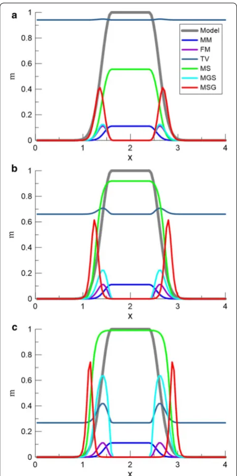
We examine how different values of β affect the stabi-lizing performance by using a simple 1D model which is given by
where x is the logarithm of the depth and has a value that changes from 0 to 4 in increments of 0.04, and mapr is
assumed to be 0 over the whole range of x. The behaviors of the different stabilizing functionals after normaliza-tion are shown in Fig. 1. We see that stabilizing function-als, such as the TV, MGS, and MSG functionfunction-als, tend to have a narrow peak around the boundary of the model parameter, indicating effective focusing. This property is expected to help us obtain a sharp image of the elec-trical interface. If the value of the focusing parameter is changed, features of the TV and MGS are significantly altered; the effect on the sharp imaging becomes weak when the focusing parameter is increased. Conversely,
(13)
over a wide range (Fig. 1). Different values of the focus-ing parameter will have different MS values, so that the position of MS boundary should change accordingly. The gradient of the MSG is calculated after the calculation of the MS, so the boundary positions of MSG are expected to change with changes in focusing parameter. Neverthe-less, it still focuses the right boundary position (x-axis from 1 to 1.5 and 2.5 to 3).
We can thus choose different optimization methods to minimize the objective functional so that inversion can be performed by using different stabilizing functionals in the same framework. In the next section, we perform synthetic tests using 1D-layered and 2D wedge models to compare the performance of inversion with different stabilizing functionals. Here, we applied Occam’s inversion (Constable et al. 1987) with a self-adaptive conjugate gradient weighted optimization scheme for 1D case. We used the ratio of data misfit and the value of each stabilizing functional as the initial value of regularization parameter, we kept the same regularization parameter if the data misfit decreases dur-ing the inversion, while we set αn+1=0.9∗αn if the data
were determined exactly as suggested in the original paper (Constable et al. 1987).
Synthetic model test One‑dimensional model
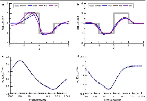
Here we test 1D models with sharp and smooth bounda-ries to observe the effect of different stabilizing function-als, i.e., smoothing functionals (MM, FM, and SM) and focusing functionals (TV, MS, MGS, and MSG). We use
80 frequencies from 1000 to 0.001 Hz for the forward cal-culation to generate synthetic data. Then, 1% Gaussian noise was added to the synthetic data and the observa-tion error was assumed also to be 1%. If we applied higher noise and error, the result of each stabilizing functional easily reached the target misfit so that all results showed little difference. Then, we calculated apparent resistivity, and a logarithmic scaling was applied.
The synthetic 1D-layered model is shown by a gray thick line in Fig. 2a (model A) and b (model B). The mod-els with opposite contrast are given by the function
and
where x is the logarithm of the depth, and it consists of one high-resistivity anomalous layer and one low-resis-tivity anomalous layer embedded in a uniform half-space with a resistivity of 100 Ω m. The resistivity and thickness of the shallower anomaly are 1000 Ω m and 0.9 km rang-ing from 0.1 to 1 km in depth, and those of the deeper anomaly are 10 Ω m and 9 km ranging from 1 to 10 km. The common boundary of the two anomalous layers is 1 km (x = 0) in depth. The synthetic sounding curve of each model is shown in Fig. 2c, d. The model is discre-tized into 40 layers, and the maximum depth is 100 km.
The initial model is a 100-Ω m uniform half-space, and the a priori model is the same as the initial model. The dependence on the starting model is mainly from the dif-ferent optimization methods to minimize the objective functional. Here we use Occam’s inversion method to solve the inverse problem whose solution is well known to be affected little by the choice of the initial model. The choice of a priori model, mapr, is independent from the
choice of the initial model. It was confirmed that Occam’s inversion is stable so far as mapr is not too far from the
true background value (100 Ω m in this case).
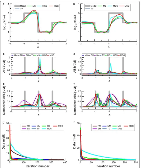
We calculated the vertical gradient of model parame-ters to determine the position and sharpness of the inter-face (Fig. 3c, d). To evaluate how the model responses fit the synthetic data, we define the root-mean-square (RMS) data misfit as
Fig. 1 Comparison of mathematical model distributions of different stabilizing functionals with square of focusing parameters β2 of a 1, b
where ND is the number of data and errj is the
observa-tion error. For Occam’s inversion, the target misfit is set to 1. Here we set the error floor equal to the assumed noise level, so it is possible to reduce RMS misfit to 1 by regularized or nonregularized inversion. However, in some cases, the solution suffered from overfitting. To evaluate how the synthetic model parameters are recov-ered by inversion, we also calculate the RMS model recovery (Zhang et al. 2012) defined as
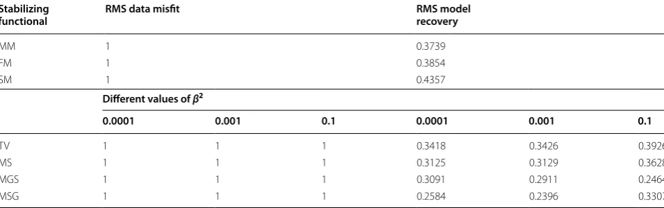
The obtained RMSd and RMSm values are given in
Tables 1 and 3. For a detailed discussion, we also sepa-rately calculated the RMS model recovery of each electri-cal boundary (for the range of x from − 1.5 to − 0.5, from
− 0.5 to 0.5, and from 0.5 to 1.5, respectively) for the two models, as given in Tables 2 and 4.
(17)
RMSm=
N k=1
minvk −mmodelk 2
N .
Both for models A and B, all inversion results reached the target misfit even with different values of β2 in both
two cases. When β2 was set to 0.1 (Fig. 3a, b), TV, MS,
MGS, and MSG had a similar RMS model recovery for model A, significantly smaller than smooth results. All of them had a better recovery for the boundary around
x = 0 (Table 2). In model B, the MGS had the small-est RMS model recovery of 0.2464. However, the RMS model recovery of the MS and MSG was also as small as 0.3628 and 0.3307, respectively, while TV had a poor RMS model recovery as 0.3926. The MGS results showed an accurate boundary at x = 0 (Fig. 3c, d), and the MSG results showed a more accurate boundary location at
x = − 1 and x = 1.
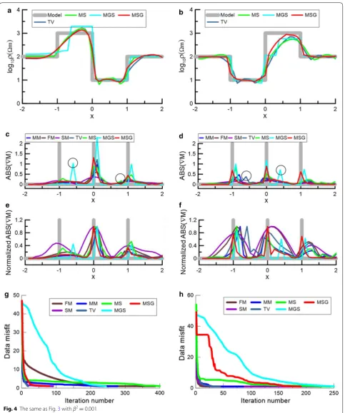
Next we varied the focusing parameter value to 0.001 and 0.0001 and observed the influence. With decreas-ing β2 to 0.001, the focusing stabilizers had a better effect
on imaging the sharp interface than those results with smooth model constraints (Fig. 4a, b). With the MSG and MGS stabilizers, the position of the boundary was imaged
Fig. 3 1D-layered model inversion results of different stabilizing functionals with β2= 0.1: a inversion results of the model A, b inversion results of
more accurately than that with the MS and TV at x = 1. At x = 0, MGS showed a more sharp boundary. However, the
MS and MGS results appear to be unstable and produce some false features around x = − 0.5 and x = 0.8 (black
circles in Fig. 4c). For model B, the MSG result had the smallest RMS model recovery of 0.2396, and it had a bet-ter performance for imaging every boundary (Fig. 4d and Table 4). However, TV and MGS produced false features
Table 1 RMS data misfit and RMS model recovery of different stabilizing functionals for the 1D-layered model A (Fig. 2a)
Stabilizing
functional RMS data misfit RMS model recovery
MM 1 0.2405
FM 1 0.2374
SM 1 0.2630
Different values of β2
0.0001 0.001 0.1 0.0001 0.001 0.1
TV 1 1 1 0.1851 0.1764 0.1825
MS 1 1 1 0.1746 0.1622 0.17585
MGS 1 1 1 0.2567 0.2318 0.2156
MSG 1 1 1 0.1769 0.1548 0.1808
Table 2 RMS model recovery around each boundary of the 1D-layered model A (Fig. 2a)
Stabilizing
functional First boundaryx from − 1.5 to − 0.5 Second boundaryx from − 0.5 to 0.5 Third boundaryx from 0.5 to 1.5
MM 0.3097 0.1798 0.1938
FM 0.2266 0.1681 0.2076
SM 0.2411 0.3479 0.2628
Different values of β2
0.0001 0.001 0.1 0.0001 0.001 0.1 0.0001 0.001 0.1
TV 0.2334 0.2279 0.2337 0.1609 0.1288 0.1684 0.2132 0.2016 0.2018 MS 0.2432 0.2159 0.2939 0.1729 0.2074 0.1677 0.1921 0.1135 0.2052 MGS 0.2880 0.2332 0.2259 0.3255 0.1905 0.1665 0.2464 0.1496 0.2054 MSG 0.2306 0.2299 0.2035 0.1342 0.1301 0.1637 0.2001 0.1205 0.2160
Table 3 RMS data misfit and RMS model recovery of different stabilizing functionals for the 1D-layered model B (Fig. 2b)
Stabilizing
functional RMS data misfit RMS model recovery
MM 1 0.3739
FM 1 0.3854
SM 1 0.4357
Different values of β2
0.0001 0.001 0.1 0.0001 0.001 0.1
TV 1 1 1 0.3418 0.3426 0.3926
MS 1 1 1 0.3125 0.3129 0.3628
MGS 1 1 1 0.3091 0.2911 0.2464
around x = − 0.5 and x = 0.5 (Fig. 4d), respectively. When
β2 was decreased further to 0.0001 (Fig. 5a, b), for model
A, the MS results produce more false features around
x = 0.5, while MGS had large model recovery because of its false features occurred around x = − 0.5 to x = 1.2. The MSG result still remains stable, accurately recovering both the resistivity values and interface depths, especially x = 0 (Fig. 5c, e). For model B, TV and MGS produced lots of false features around x = − 0.8 and x = 0.2 (Fig. 5d). From the comparison of models A and B, the boundary changing from resistive to conductive (x = 0 in Figs. 3a, 4a, 5a and
x = − 1 in Figs. 3b, 4b, 5b) is imaged more sharply than the boundary of opposite contrast.
Although the TV, MS, and MGS yield the sharp bound-aries in some cases (boundbound-aries of x = 1 in Figs. 3a, 4a and x = 0 in Figs. 3b, 4b), they also produce numerous false structures (at depths of x = − 0.5 in Figs. 4a, 5a and
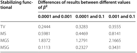
x = 0.5 in Figs. 4b, 5b), suggesting the inversion is unsta-ble due to the small value of the focusing parameter. For a given stabilizer, we also calculated the difference between each pair of inversion results produced by different β2
values (β1 and β2) as
These differences for different stabilizers are summa-rized in Tables 5 and 6. The MSG results had the smallest differences when selecting different values of β2, which
means the MSG inversion is more robust against varia-tion in β2 than those of the TV, MS, or MGS. It is a great
advantage of using the MSG stabilizer that fine-tuning of
β2 is not necessary to obtain a stable solution.
The third 1D synthetic model shows spatially smooth variation in the electrical conductivity and is represented
(18)
Thus, the anomaly changes at the logarithm depths ranging from 0.1 to 0.5 km and from 2.5 to 10 km in a background resistivity of 10 Ω m. The initial and a priori models are both in a 10-Ω m half-space.
The inversion results from each stabilizing functional with different β2 values are shown in Fig. 6. The data
misfit and model recovery are given in Table 7. The TV, MS, MGS, and MSG results have discontinuities where the synthetic model parameters change smoothly. The FM and SM results show excellent performance for con-ductive anomaly, as their RMS data misfit values both reached 1 and their RMS model recovery values became small, reaching 0.1707 and 0.1744, respectively. Thus, the results imply that the FM or SM is a better choice for cases with smooth boundaries, although results using all focusing stabilizers also show an acceptable performance both in terms of RMS misfit and model recovery.
Two‑dimensional wedge model
For further discussion, we test all five stabilizing func-tionals using 2D synthetic models with a resistive and conductive wedge (Fig. 7a, b). The 2D wedge model con-figuration is the same as that used by de Groot-Hedlin and Constable (2004) and Zhang et al. (2009). The upper boundary of the wedge has a slope of 5.7°, and the lower boundary has a slope of 16.6°. In total, 24 synthetic observation sites are distributed regularly at intervals of
(19)
Table 4 RMS model recovery around each boundary of the 1D-layered model B (Fig. 2b)
Stabilizing
functional First boundaryx from − 1.5 to − 0.5 Second boundaryx from − 0.5 to 0.5 Third boundaryx from 0.5 to 1.5
MM 0.1521 0.6164 0.3741
FM 0.1329 0.6625 0.3257
SM 0.1851 0.7233 0.4128
Different values of β2
0.0001 0.001 0.1 0.0001 0.001 0.1 0.0001 0.001 0.1
0.5 km. For the modeling, 92 mesh grids are defined in the horizontal direction with a 0.125-km spacing, and 100 layers are set in the vertical direction, which is dis-cretized with the same increment. We used the finite-element code in Occam’s inversion for the modeling. The mesh spacing for the inversion is set twice as large as that in the forward modeling, using 46 meshes in the horizon-tal direction and 50 layers in the vertical direction. We used 20 frequencies from 4 to 0.0063 Hz for the resistive wedge model and 24 frequencies from 400 to 0.01 Hz for the conductive wedge model to perform the modeling that generates synthetic data (de Groot-Hedlin and Con-stable 2004). Both transverse electric (TE) and transverse magnetic (TM) modes were used in the calculation. The synthetic sounding curves of apparent resistivity and phase from site 10 (red triangle in Fig. 7a) of the resistive wedge case are shown in Fig. 8 as an example.
In the 2D resistive wedge model, the background resistivity is 1 Ω m and that of the wedge-shaped body is 100 Ω m. We allow the resistivity values to change from 0.01 to 500 Ω m during the inversion. The start-ing model is a 1-Ω m half-space, and the a priori model is also a 1-Ω m uniform half-space. Again, the different initial model affects little, and the regularization works well when a priori model is not too far from the true
background resistivity (1 Ω m in this case). We add 1% random noise in the synthetic data and set the error floor as 1% in the inversion. Then, it is not easy to get the data misfit small. We also tried cases with larger error floor. In those cases, it was quite easy to get data misfit down, but resulting model was much less sharp than the present
Table 5 Differences [calculated using Eq. (18)] between the inversion results of model A (Fig. 2a) obtained using different values of β2
Stabilizing func‑
tional Differences of results between different values of β2
0.0001 and 0.001 0.0001 and 0.1 0.001 and 0.1
TV 0.2444 0.3283 0.3555 MS 0.5981 0.4469 0.8141 MGS 1.8372 1.2791 2.1665 MSG 0.1113 0.2327 0.3431
Table 6 Differences (calculated using Eq. (18)) between the inversion results of model B (Fig. 2b) obtained using different values of β2
Stabilizing func‑
tional Differences of results between different values of β2
0.0001 and 0.001 0.0001 and 0.1 0.001 and 0.1
TV 0.2033 0.3971 0.3547 MS 0.5877 0.4114 0.3338 MGS 0.9131 1.8126 2.0463 MSG 0.1949 0.2099 0.2951
results. It depends on the noise and error given to the synthetic data whether we can easily get the data misfit down to an RMS value of 1.
We calculated the RMS data misfit and the model recovery, the definitions of which are the same as in the 1D case (Table 8). The inversion using the smooth
stabilizing functionals, such as the MM (Fig. 9a), FM (Fig. 9b), and SM (Fig. 9c), reached the target misfit, and their RMS model recovery values are reduced only a lit-tle to 0.4584, 0.3583, and 0.3456, respectively. This means that none of these stabilizing functionals helps yield the right shape and value of the wedge. Here the result with TV is not shown because the inversion did not converge, and most probably because the TV stabilizer constrains L1 norm of the spatial gradient, which is not consistent
with the framework of Occam’s inversion with L2 norm.
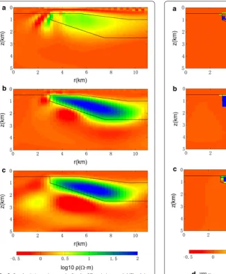
Results using focusing (MS, MGS, and MSG) function-als and variations for different focusing parameters are shown in Figs. 10, 11, 12. They are generally better than the results using smooth constraints (Table 8). We then compared the results using different focusing parameters. When β2 is 0.0001, the MS result (Fig. 10a) has a model
recovery of 0.4302 and shows some false structures below the wedge. As a whole, the shape of the wedge body is not restored well. The MGS (Fig. 10b) and MSG results (Fig. 10c) both have smaller RMS model recovery values (0.3242 and 0.2499, respectively) than those of the results with smooth constraints. However, the bottom boundary of the wedge for the MGS result is not as accurate as that for the MSG result.
If β2 is increased to 0.001, each inversion result
var-ies in different degrees. The MS (Fig. 11a) and MGS results (Fig. 11b) exhibit considerable changes. Both of them perform better than previous results in terms of the model recovery (0.2983, 0.3164, respectively). The results of the MSG stabilizer (Fig. 11c) are more stable and acceptable than those of other stabilizing function-als, as they reached the target misfit and achieved the smallest model recovery (0.2634). Further increasing β2
to 0.1, the MS and MGS results changed drastically, but the MSG results still achieve stability and remain the best among results using different functionals (model recov-ery of 0.3005). Additionally, the MS (Fig. 12a) and MGS
Table 7 RMS data misfit and RMS model recovery of different stabilizing functionals for 1D smooth boundary model
Stabilizing
functional RMS data misfit RMS model recovery
MM 1 0.2528
FM 1 0.1707
SM 1 0.1744
Different values of β2
0.0001 0.001 0.1 0.0001 0.001 0.1
TV 1 1 1 0.2353 0.2260 0.2899
MS 1 1 1 0.2402 0.2617 0.1992
MGS 1 1 1 0.2267 0.2616 0.1877
MSG 1 1 1 0.2105 0.1839 0.2160
results (Fig. 12b) produced some false structures, in both the shape and resistivity of the wedge. Conversely, the MSG results (Fig. 12c) successfully reproduced the shape and the resistivity of the wedge. As a whole, the MSG stabilizer shows the best performance as can be seen in a general view of the RMS model recovery with different focusing parameters (Fig. 13).
Thus, the MSG stabilizing functional was shown to be able to not only describe the sharp boundary but also estimate the model parameter more accurately than other functionals. In addition, it is very stable in the regular-ized inversion and is influenced by the focusing param-eter value much less than the MS and MGS stabilizers.
Fig. 8 Synthetic 2D apparent resistivity and phase curves of site 10 for the resistive model: a TE apparent resistivity, b TE phase, c TM apparent resistivity, and d TM phase. Observation errors corresponding to 1% of impedance amplitude are also shown
Table 8 RMS data misfit and RMS model recovery of different stabilizing functionals for 2D resistive model
Stabilizing functional RMS data misfit RMS model recovery
MM 1 0.4584
FM 1 0.3583
SM 1 0.3456
Different values of β2
0.0001 0.001 0.01 0.0001 0.001 0.01
MS 1 1 1 0.4302 0.2983 0.3243
MGS 1 1 1 0.3242 0.3164 0.3842
We also performed synthetic tests for a 2D conduc-tive wedge model (Fig. 7b). Figure 14 shows a result of inversion using the MSG regularization. Again we can conclude that the MSG stabilizer provides a good perfor-mance among all stabilizers tested. The synthetic inver-sion results for 1D case in “One-dimensional model” section showed that MT is insensitive to the sharpness in the vertical direction. The 2D results are sharper than 1D results, indicating that the sharpness of inclined interface of 2D cases is mostly due to the horizontal gradient.
Conclusion
In this paper, to consider the stability on sharp bounda-ries, we proposed a new stabilizing functional called the MSG stabilizing functional for imaging sharp interfaces
of resistivity structure by magnetotelluric inversion. We compared its performance with other stabilizers under the same inversion framework through the uni-fied objective functional form of a discrete weighted matrix. By comparing 1D and 2D synthetic inversed results using different stabilizers, we confirmed that the
Fig. 9 Synthetic inversion results for the 2D resistive model (Fig. 6a) using different stabilizing functionals a MM, b FM, and c SM. Color scale is the same as Fig. 6a
MSG stabilizer was not only able to resolve a geoelectri-cal interface but also stable for a wide range of the focus-ing parameter value. The MSG stabilizer also showed
good performance regarding both data misfit and model recovery from synthetic data inversion with sharp boundaries. The overall results of the present study
Fig. 11 Synthetic inversion results for the 2D resistive model (Fig. 6a) using different stabilizing functionals with β2= 0.001: a MS, b MGS, c
MSG results, and d convergence of RMS data misfit. Color scale is the same as Fig. 6a
Fig. 12 Synthetic inversion results for the 2D resistive model (Fig. 6a) using different stabilizing functionals with β2= 0.01: a MS, b MGS, c
Fig. 13 The model recovery curve with different focusing parameters for the 2D resistive model (Fig. 6a)
Fig. 14 A synthetic (a) inversion result with the MSG stabilizer for the 2D conductive wedge model (Fig. 6b). Color scale is the same as that in Fig. 6b
suggest that this stabilizing functional would be effective in practical applications.
Abbreviations
MT: magnetotelluric; MS: minimum support; MGS: minimum gradient support; MSG: minimum support gradient; 1D: one-dimensional; 2D: two-dimensional; RRI: rapid relaxation inversion; REBOCC: reduced basis Occam’s inversion; NLCG: nonlinear conjugate gradients; TV: total variation; MM: the minimum model; FM: the flattest model; SM: the smoothest model; RMS: the root-mean-square; TE: transverse electric; TM: transverse magnetic.
Authors’ contributions
YX completed all the tests, words, diagrams, and discussion of this study, PY proposed the method and was responsible for the manuscript, LL and SK contributed to the part of discussion, and HU leaded the whole discussion, improvement, and all the corrections in detail. All authors read and approved the final manuscript.
Author details
1 State Key Laboratory of Marine Geology, Tongji University, 1239 Siping Road, Shanghai 200092, China. 2 Earthquake Research Institute, University of Tokyo,
1-1-1, Yayoi, Bunkyo-ku, Tokyo 113-0032, Japan. 3 School of Naval Architecture, Ocean and Civil Engineering, Shanghai Jiaotong University, Shanghai 200240, China.
Acknowledgements
The present research was partially supported by Chinese National Natural Science Foundation (41774123, 41506053), Chinese National Key Research and Development Program (2016YFC0601104), National Science and Technol-ogy Major Project (2016ZX05004-003, 2016ZX05027-001-008), Independent Project from State Key Laboratory of Marine Geology (Tongji University) (MG20170204), Strategic Leading Science and Technology Project, Chinese Academy of Sciences (B Class) (XDB10030500), the China Scholarship Council, and the Earthquake Research Institute of the University of Tokyo. We are grate-ful to Dr. Spitzer, Dr. Farquharson and anonymous referees for their important comments that enabled us to improve the manuscript significantly.
Competing interests
The authors declare that they have no competing interests.
Availability of data and materials
All the data and models in this manuscript are available.
Consent for publication Not applicable.
Ethics approval and consent to participate Not applicable.
Received: 2 March 2017 Accepted: 7 November 2017
References
Acar R, Vogel CR (1994) Analysis of total variation penalty methods. Inverse Prob 10:1217–1229
Constable SC, Parker RL, Constable CG (1987) Occam’s inversion: a practical algorithm for generating smooth models from electromagnetic sound-ing data. Geophysics 52:289–300
de Groot-Hedlin C, Constable SC (1990) Occam’s inversion to generate smooth, two-dimensional models from magnetotelluric data. Geophysics 55:1613–1624
de Groot-Hedlin C, Constable SC (2004) Inversion of magnetotelluric data for 2D structure with sharp resistivity contrasts. Geophysics 69:78–86 Farquharson CG (2008) Constructing piecewise-constant models in
multidi-mensional minimum-structure inversions. Geophysics 73(1):K1–K9 Farquharson CG, Oldenburg DW (1998) Non-linear inversion using general
measures of data misfit and model structure. Geophys J Int 134:213–227 Fournier HG, Febrer J (1976) Gaussian character of the distribution of magne-totelluric results working in log-space. Phys Earth Planet Inter 12:359–364 Grayver AV, Kuvshinov AV (2016) Exploring equivalence domain in nonlinear
inverse problems using Covariance Matrix Adaption Evolution Strategy (CMAES) and random sampling. Geophys J Int 205:971–987
Last BJ, Kubik K (1983) Compact gravity inversion. Geophysics 48:713–721 Marcuello-Pascual A, Kaikkonen P, Pous J (1992) 2-D inversion of MT data with
a variable model geometry. Geophys J Int 110:297–304
Portniaguine O, Zhdanov MS (1999) Focusing geophysical inversion images. Geophysics 64:874–887
Rodi W, Mackie RL (2001) Nonlinear conjugate gradients algorithm for 2-D magnetotelluric inversion. Geophysics 66:174–187
Rudin LI, Osher S, Fatemi E (1992) Nonlinear total variation based noise removal algorithms. Physica D 60:259–268
Siripunvaraporn W, Egbert G (2000) An efficient data-subspace inversion method for 2-D magnetotelluric data. Geophysics 65:791–803 Smith JT, Booker JR (1991) Rapid Inversion of two and three dimensional
magnetotelluric data. J Geophys Res 96:3905–3922
Smith T, Hoversten M, Gasperikova E, Morrison F (1999) Sharp boundary inver-sion of 2D magnetotelluric data. Geophys Prospect 47:469–486 Tikhonov AN, Arsenin VY (1977) Solution of ill-problems. Winston and Sons,
Uchida T (1993) Smooth 2-D inversion for magnetotelluric data based on statistical criterion ABIC. J Geomagn Geoelectr 45:841–858
Weaver JT, Agarwal AK, Lilley FEM (2000) Characterization of magnetotelluric tensor in terms of its invariants. Geophys J Int 141:321–336
Zhang LL, Yu P, Wang JL, Wu JS (2009) Smoothest model and sharp bound-ary based two-dimensional magnetotelluric inversion. Chin J Geophys 52:1625–1632
Zhang LL, Yu P, Wang JL, Wu JS, Chen X, Li Y (2010) A study on 2D magnetotel-luric sharp boundary inversion. Chin J Geophys 53:631–637
Zhang LL, Koyama T, Utada H, Yu P, Wang JL (2012) A regularized three-dimensional magnetotelluric inversion with a minimum gradient support constraint. Geophys J Int 189:296–316
Zhdanov MS (2002) Geophysical inverse theory and regularization problems. Elsevier, Amsterdam
Zhdanov MS (2004) Minimum support nonlinear parametrization in the solu-tion of a 3D magnetotelluric inverse problem. Inverse Prob 20:937–952 Zhdanov MS (2009) New advances in regularized inversion of gravity and
electromagnetic data. Geophys Prospect 57:463–478