Variable Fidelity Surrogate Assisted Optimization
Using a Suite of Low Fidelity Solvers
Mohammad Kashif Zahir, Zhenghong Gao
School of Aeronautics, Northwestern Polytechnical University, Xi’an, China Email: [email protected]
Received July 10, 2012; revised August 22, 2012; accepted September 17, 2012
ABSTRACT
Variable-fidelity optimization (VFO) has emerged as an attractive method of performing, both, high-speed and high- fidelity optimization. VFO uses computationally inexpensive low-fidelity models, complemented by a surrogate to ac-count for the difference between the high- and low-fidelity models, to obtain the optimum of the function efficiently and accurately. To be effective, however, it is of prime importance that the low fidelity model be selected prudently. This paper outlines the requirements for selecting the low fidelity model and shows pitfalls in case the wrong model is cho-sen. It then presents an efficient VFO framework and demonstrates it by performing transonic airfoil drag optimization at constant lift, subject to thickness constraints, using several low fidelity solvers. The method is found to be efficient and capable of finding the optimum that closely agrees with the results of high-fidelity optimization alone.
Keywords: Variable Fidelity; Airfoil Optimization; Surrogate Models
1. Introduction
Given the high cost of CFD and optimization, a promi- nent area of research today is to find ways to reduce the computational time while retaining the high-fidelity of the analysis. In the area of aerodynamic optimization, the variable fidelity (also called multifidelity) method has quickly grown in popularity [1-7].
Variable-fidelity and other model management me- thods have been developed to solve optimization prob- lems that involve simulations with large computational ex- pense [4,8]. In many engineering design problems, dif- fering levels of fidelity can model the system of interest. Higher-fidelity models typically incorporate more detail- ed physics and are computationally expensive to evaluate
than lower fidelity models. The lower-fidelity models are
typically much cheaper to evaluate, but designs produced by using these models neglect important physical effects
included in the more expensive higher-fidelity models. In
aircraft design, Navier-Stokes and Euler equations are examples of two computational models with different
fidelity.
Variable-fidelity optimization has emerged as an at- tractive method of performing, both, high-speed and high- fidelity optimization [1-9]. These algorithms attempt to le- verage information from computationally inexpensive low- fidelity models to reduce the time required to converge to the optimum of the high-fidelity function. This is usually accomplished by building a computationally inexpensive surrogate for the high-fidelity model. The surrogate is, often, iteratively optimized and updated as new high-
fidelity data become available. In variable-fidelity algo- rithms, the surrogate for the high-fidelity model usually consists of the low-fidelity model plus a correction term that models the difference between the high- and low- fidelity models, calibrated at selected sample points in the design space [7].
The variable-fidelity method has its roots in the em- pirical model-building theory—the idea of endowing a surrogate with some discipline related properties to in- crease its accuracy-and the past three decades have seen rapid increase in its development and use [10]. Insightful reviews of the variable-fidelity method can be found in [8,10]. The method has improved immensely; from its initial form requiring Taylor polynomials [1], to its cur- rent incarnation using a variety of modern surrogate mo- dels like Kriging and neural networks [4,9]; and from using a variety of multiplicative, additive and hybrid cor- rections [4], to the method of Co-Kriging [3]. In the opti- mization context, the method has been used in both derivative-based [1] and derivative free [11] optimiza- tion.
ral low fidelity solvers.
This paper is arranged as follows: first the major tech- nology pieces used in the design are described; next, the VFO framework is presented followed by the results of the optimization. The VF optimization results are also compared to the results of direct optimization—where the HF solver, alone, was coupled to the optimizer to find the optimum result.
2. Design Tools
2.1. Flow Solver
In this study, the RAE-2822 airfoil was chosen for op- timization. Two flow solvers were used: 1) XFOIL, a simple linear-vorticity stream function panel method with an integral boundary layer formulation to account for viscous effects [12], and 2) an indigenously deve- loped 2D compressible Navier-Stokes solver—using the LU-SGS time stepping scheme, the Roe upwind scheme and multigrid acceleration—capable of being used in, both, Euler and Navier-Stokes mode [13]. XFOIL, Euler, and low resolution (small grid) Navier-Stokes solvers were used as the LF solvers, while Navier-Stokes with
the K-ωturbulence model was used as the HF solver.
The Euler and Navier Stoker solvers used a C-type mesh extending 20 chord lengths downstream of the
trailing edge. The first grid line was 2 × 10⁻⁶ units from
the airfoil surface for the Navier-Stokes solver and 0.01 units for the Euler solver. The HF solver used a grid size of 216 cells around the airfoil and 44 cells normal to the airfoil (216 × 44 grid), selected after obtaining good agreement in the surface pressure distribution and aero- dynamic coefficients at transonic conditions (Mach num-
ber of 0.729, Reynolds number of 6.5 × 10⁶ and an angle
of attack of 2.31˚) as reported in [14,15]
2.2. Optimization Algorithm
A genetic algorithm (GA) was used to perform the opti- mization in this study. GA searches from multiple points in the design space, instead of moving from a single point like gradient-based methods do making it less prone to being trapped by local optima. This makes it particularly suitable for aerodynamic optimization where the function landscape is often multimodal and nonlinear
because the flow field is governed by a system of non-
linear partial differential equations [16]. Furthermore, GA works on function evaluations alone and does not require derivatives or gradients of the objective function. These features make it a robust global optimization algorithm.
The GA implementation in MATLAB and its optimi- zation toolbox was used to perform the optimization.
2.3. Sample Plan
As with all surrogate-based methods, to approximate a
function f we start with a set of sample data—computed
at a set of points in the domain of interest determined by a sampling plan. Selection of the sample points is a very important step towards creating a good surrogate model. If the sample plan model is too sparse or does not contain the interesting features of the design space, the resulting model will fail to resolve desirable global features. In order to improve the surrogate it is necessary to incre- mentally add points in an intelligent way such that the generated surface converges toward the true surface.
When dealing with large, complex design spaces, it is often unclear how many points may be necessary to re- solve key features with a response surface. To get the maximum amount of information out of a minimum number of points with no a priori knowledge of the de- sign space requires uniform sampling.
Several sampling methods are capable of producing relatively uniform samples, e.g. Latin Hypercube samp- ling [17], however not many methods allow incremental
uniform sampling. Latin Hypercube sampling requires a
priori knowledge of how many points are desired in order to divide the domain into the appropriate number of hypercubes. This method creates nearly uniform point distributions, but requires a completely new set of data if additional points are desired. Another sampling method known as the Sobol Sequence [18] has good space filling properties and allows incremental uniform sampling [6, 17]. This method was, thus, adopted in this study to create the sample plan. Since the number of sample points required to obtain an accurate surrogate is gene-
rally unknown a priori, an initial sample of 10 nvar
(where nvar is the number of design variables) was
created following the suggestion of Jones et al. [19].
2.4. Surrogate Model
The surrogate model used in the study was Kriging—an approximation technique that has received much atten- tion in recent years [2-6,8,9,19,20]—named after the pio- neering work of the South African mining engineer D. G. Krige and introduced in engineering design work after the seminal paper by Sacks et al. [20].
For brevity, the Kriging equations are not mentioned here. Forrester el al. [17] contains more detail about Kri- ging.
The Kriging model in this study used a constant reg-
ression term and a Gaussian correlation model. The p
term was 2 for all dimensions and the θ was optimized in
the range 10–2≤θi≤ 200, i = 1, 2, ···, nvar. The surrogate model were created using the surrogates toolbox [21] for MATLAB.
3. Design Variables
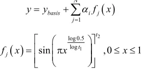
airfoil geometry is then modified by adding smooth per- turbations in the form of the Hicks-Henne bump func- tions [22]. The Hicks-Henne shape function modifies airfoil geometry by adding a linear combination of shape functions, fj and weighting coefficients, αjas follows:
1N
basis i j
j
y y f x
2
1
log 0.5 log
sin ,0 1
t
t j
f x x x
Here t1 locates the maximum point of the bump and t2
controls the width of the bump. The design variables are
the coefficients αj multiplying the various Hicks-Henne
bump functions.
In this study, 7 bump functions were used for the up- per and lower surface of the airfoil, resulting in a total of
14 design variables. The points t1 were linearly spaced
between 0 and 0.94. The range was terminated a little before the trailing edge to prevent the upper and lower edges from crossing each other and creating unrealistic
geometries. A value of 10 was used for t2 following Cas-
tonguay’s [23] recommendation.
To prevent large changes to the geometry, upper and
lower bounds were set on αj. These were: –0.005 ≤ αj≤
0.005, j =1, 2 and 13, 14, –0.01 ≤αj≤ 0.01 otherwise.
4. Fitness Function and Constraints
This was a single objective optimization problem. The airfoil was optimized for a transonic Mach number of
0.729 and a fully turbulent Reynolds number of 6.5 × 10⁶.
The objective was to minimize the drag, cd at a constant
lift, cl = 0.6 ± 0.01. The constant lift constraint was
maintained by varying the angle of attack, α, of the air-
foil. At low to moderate values of α, i.e. before flow
separation and stall, cl varies linearly with α. During each evaluation of the fitness function, the airfoil is first si- mulated at an initially guessed α1 and at α2. A third si-
mulation at α3, found from a linear interpolation through
(α1, cl1) and (α2, cl2), is then used to attain the desired lift.
This procedure effectively removes the cl constraint from
the optimization by making it a condition which each
simulation must satisfy. The optimization is simplified
both by the removal of the constraint and by reducing the
dimensionality of the problem, since αis not used as an
optimization variable. The airfoil thickness to chord ratio,
t c max was required to be greater than 12.11% (the
max of the initial airfoil). The thickness constraintwas imposed by adding a penalty term to the fitness function. The final fitness function was:
t c
*max max 0,
l
d c const
f x c t c t c
where
t c * was the minimum allowable thickness of12.11%.
5. The VFO Framework
A variable fidelity prediction predicts the function res- ponse in 2 steps: 1) the low fidelity function is evaluated to obtain an estimate; 2) the estimate is corrected by performing a high fidelity simulation to obtain a better estimate to the function and apply a correction to the low fidelity prediction. The correction between the high and low fidelity functions is modeled by a surrogate model developed by sampling the function at a few points. To evaluate the goodness of fit over the entire function
landscape, the RMSE and R2 of the surrogate is cal-
culated for a validation dataset generated using a uniform
Latin Hypercube sample consisting of ntest = nvar × 10
[image:3.595.103.241.154.222.2]points.
Figure 1 shows the flowchart of the VFO framework
used in this study. If the initial number of points used to construct the surrogate do not result in an accurate surrogate, the surrogate is updated by adding more points until some accuracy criteria is satisfied. The surrogate is then directly coupled to the GA to determine the opti- mum.
It has been reported that when a surrogate is used for
fitness evaluation, it is very likely that the evolutionary
algorithm will converge to a false optimum [24]. A false optimum is an optimum of the approximate model, which is not one of the original fitness function. To avoid this, the VF optimum point was evaluated by the HF solver every 10 generations. If the VF lift coefficient, cl, agreed with the HF cl prediction within a 0.01 tolerance, and the drag coefficient within 0.0001, the optimization was con- tinued. Otherwise, the surrogate model was updated by performing HF evaluations on the GA population and refitting the surrogate before continuing the optimization.
6. Results and Discussion
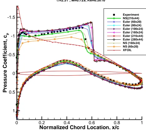
Use of XFOIL, Euler and Navier-Stokes solvers with se- veral grid sizes was investigated for use as the low- fidelity solvers. The surface pressure distribution on the RAE-2822 at Mach number of 0.729, Reynolds number
of 6.5 × 10⁶ and an angle of attack of 2.31˚ are show in
Figure 2. Results of the HF solver (NS 216 × 44) are
also shown. All Navier Stokes solvers used the K-ω
turbulence model and an initial grid line spacing of 2 × 10⁻⁶ units from the airfoil surface. The Euler solvers used
an initial grid line spacing of 0.01units from the airfoil
surface. Difference between the aerodynamic coefficients of the low-fidelity solvers and the HF solver is shown in
Figure 3. The computation time for one run is also
shown.
Figure 2 shows that all solvers, except XFOIL, follow
Figure 1. The VFO framework.
distribution. XFOIL, being incapable of analyzing shocked flows, does not predict a shock wave. However, the aerodynamic lift and drag coefficients are surprisingly close to the HF solver predications.
Pressure Distribution on RAE-2822 for Low and High Fidelity Solvers
=2.31o
, M=0.729, Re=6.5x10⁶
+ + + + + + + + + + + + + + + + + + + + + + + + + + + + + + + + + + + + + + + + + + + + + + + + + + + + + + + + + + + + + + + + + + + + + + + + + + + ++ +++ ++ ++ +++ +++ + +++ +++ + + + + + + + + + + + ++ + + + ++ + + + +++++++ ++++ Experiment NS(216x44) Euler (60x20) Euler (80x24) Euler (100x24) Euler (160x24) Euler (216x44) Euler (280x44) NS (160x24) NS (60x20) XFOIL -1.5
Normalized Chord Location, x/c
P res su re C o e ff ic ie nt ,
cp -1
+ -0.5 0 0.5 1
[image:4.595.304.536.94.305.2]0 0.2 0.4 0.6 0.8 1
Figure 2. RAE-2822 airfoil surface pressure distribution for the high and low fidelity solvers. Experimental data for the selected case is also shown for reference.
Difference between Low and High Fidelity Results
% di fferen c e fr om N S (216 × 44) ti me s ( s)
Figure 3. Difference between the aerodynamic coefficients of the LF solvers and the HF solver. Solver runtime is also shown.
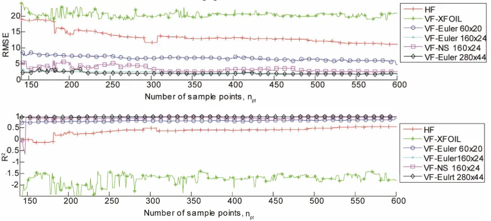
Five LF solvers were selected for the VF surrogate in this study to cover the entire spectrum from slow to fast and less accurate to more accurate: XFOIL, Euler 60 ×20,
Euler 160 × 24, Euler 280 × 44 and NS 160 × 24. Figure
4 shows the RMSE and R2 values for the Kriging sur-
rogate fitted to the difference between the HF and LF
response, Δf, and compared to the validation dataset. A
surrogate created using the HF data alone is also shown for reference. It is immediately obvious that the VF- XFOIL surrogate is inappropriate for use in optimization:
the RMSE is too high and the R2 value is too far from the
[image:4.595.308.544.364.505.2]optimum point in some cases. This occurred because the surrogate model was updated, after every 10 generations of the GA, by performing HF evaluations on the po- pulation and adding the results to the surrogate training dataset. When one of these new training points was also an optimum point, the VF and HF yielded the same result.
predicted by the LF solver should be consistent with that of the HF solver for it to be useful in the VFO context. The XFOIL surrogate was inaccurate as XFOIL could not predict the actual aerodynamic behavior of the airfoil (at the given flow conditions) as seen in Figure 2.
The other four VF surrogates, that yielded high R2 val-
ues, were used to perform the optimization. The number of sample points used to create the VF surrogate were such that the R2 > 0.9. The optimization results are given
in Table 1 along with optimization time. HF evaluations
of the aerodynamic coefficients at the VF optimums are also reported.
It is clear from Table 1 that the NS 160 × 24 solver
yields the best lift-to-drag ratio, k, within 1% of the direct optimization result. Other solvers perform well too;
yielding k within 6% of the direct optimization result,
while still providing a significant saving in computation time. All solvers also satisfy the thickness constraint (t/c)max≥ 12.11%.
[image:5.595.56.535.273.489.2]It may appear to be surprising that the VF and HF solvers yielded the same aerodynamic coefficients at the
[image:5.595.60.540.541.737.2]Figure 4. RMSE and R2 for VF Kriging surrogate using several LF solvers.
Table 1. Aerodynamic coefficients of the baseline RAE2822 airfoil along with the optimized results using VFO with several LF Solvers. High fidelity evalutions at the VF optimum points is also shown along with total optimization time.
VF optimum result
HF evaluation at VF optimum Point Configuration
cl cd cl cd K
(t/c)max
Surrogate crea-tion time (simulations + fitting) (hours)
Optimization time (including surrogate update)
(hours)
Total time (hours)
Hours saved (compared to direct
optimiza-tion) VF, Euler 60 × 20,
599 samples 0.5984 0.00653 0.5984 0.00653 91.6774 12.37% 13.17 4.08 17.25 38.63
VF, Euler 160 × 24,
141 samples 0.5983 0.00653 0.5983 0.00653 91.5688 12.23% 3.52 6.44 9.96 45.92
VF, NS 160 × 24,
148 samples 0.5970 0.00587 0.6010 0.00637 94.3757 12.11% 4.56 10.84 15.40 40.49
VF, Euler 280 × 44,
141 samples 0.6021 0.00698 0.6061 0.00691 87.7085 12.20% 4.62 38.40 43.02 12.86
HF (direct
optimization) 0.6004 0.00643 93.4517 12.19% 55.89
Baseline RAE2822
The Euler 280 × 44 was the most computationally in- tensive LF solver used in this study, and thus expectedly, provided the least amount of time savings.
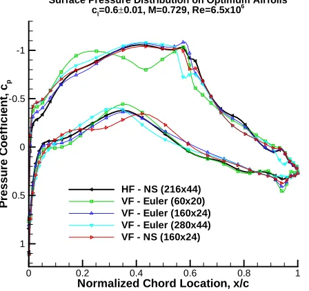
The surface pressure distributions on the optimum
airfoils are shown in Figure 5 and the airfoil geometries
are shown in Figure 6. It is seen that the optimum
pressure distributions and airfoil geometries produced using different LF solvers are quite similar. This is also reflected in the aerodynamic coefficients shown pre- viously in Table 1.
Normalized Chord Location, x/c
P
ressu
re
C
o
e
ff
ic
ie
nt,
cp
0 0.2 0.4 0.6 0.8 1
-1
-0.5
0
0.5
1
HF - NS (216x44) VF - Euler (60x20) VF - Euler (160x24) VF - Euler (280x44) VF - NS (160x24)
Surface Pressure Distribution on Optimum Airfoils
cl=0.60.01, M=0.729, Re=6.5x10
[image:6.595.64.288.222.433.2]6
Figure 5. Surface pressure distributions on the optimum airfoils. Results were calculated using the HF solver on the geometry produced by the VF optimization algorithm. The pressure distribution obtained by direct optimization using the HF solver is also shown.
Normalized Chord Location, x/c
y
/c
0 0.2 0.4 0.6 0.8 1
-0.05 0 0.05
RAE-2822 HF - NS (216x44) VF - Euler (60x20) VF - Euler (160x24) VF - Euler (280x44) VF - NS (160x24)
Comparison of Optimum Airfoils
Figure 6. Geometry of the optimum airfoils. Airfoil pro- duced by direct optimization using the HF solver, and the baseline RAE-2822 is also shown.
7. Conclusion
It can be concluded that Euler and Navier-Stokes solvers evaluated on low resolutions grids are good candidates for LF solvers as their evaluations are consistent with the HF solver. In our case, the airfoil surface pressure dis- tribution was a good means of checking the aerodynamic behavior of all candidate solvers. The VFO method used in this study is, both, efficient and capable of finding the optimum that closely agrees with the results of high- fidelity optimization alone.
REFERENCES
[1] N. M. Alexandrov, C. R. Gumbert, L. L. Green, P. A. Newman and R. M. Lewis, “Approximation and Model Management in Aerodynamic Optimization with Vari- able-Fidelity Models,” Journal of Aircraft, Vol. 38, No. 6, 2001, pp. 1093-1101. doi:10.2514/2.2877
[2] A. I. J. Forrester, N. W. Bressloff and A. J. Keane, “Op- timization Using Surrogate Models and Partially Conver- ged Computational Fluid Dynamics Simulations,” Pro- ceedings of the Royal Society A: Mathematical, Physical and Engineering Science, Vol. 462, No. 2071, 2006, pp. 2177-2204.
[3] A. I. J. Forrester, A. Sóbester and A. J. Keane, “Multi- Fidelity Optimization via Surrogate Modelling,” Proceed- ings of the Royal Society A: Mathematical, Physical and Engineering Science, Vol. 463, No. 2088, 2007, pp. 3251- 3269.
[4] S. Gano, J. Renaud and B. Sanders, “Hybrid Variable Fidelity Optimization by Using a Kriging-Based Scaling Function,” AIAA Journal, Vol. 43, No. 11, 2005, pp. 2422-2433. doi:10.2514/1.12466
[5] A. J. Keane, “Wing Optimization Using Design of Expe- riment, Response Surface, and Data Fusion Methods,” Journal of Aircraft, Vol. 40, No. 4, 2003, pp. 741-750. doi:10.2514/2.3153
[6] A. Nelson, J. Alonso and T. Pulliam, “Multi-Fidelity Ae- rodynamic Optimization Using Treed Meta-Models,” 25th AIAA Applied Aerodynamics Conference, Miami, 25-28 June 2007.
[7] S. G. Lehner, L. B. Lurati, S. C. Smith, G. C. Bower, E. J. Cramer, W. A. Crossley, F. Engelson, I. Kroo, S. C. Smith and K. E. Willcox, “Advanced Multidisciplinary Optimization Techniques for Efficient Subsonic Aircraft Design,” 48th AIAA Aerospace Sciences Meeting Includ-ing the New Horizons Forum and Aerospace Exposition, Orlando, 4-7 January 2010.
[8] D. Huang, T. Allen, W. Notz and R. Miller, “Sequential Kriging Optimization Using Multiple-Fidelity Evalua- tions,” Structural and Multidisciplinary Optimization, Vol. 32, No. 5, 2006, pp. 369-382.
doi:10.1007/s00158-005-0587-0
[image:6.595.62.280.505.699.2]doi:10.1023/A:1023283917997
[10] T. W. Simpson, V. Toropov, V. Balabanov and F. A. C. Viana, “Design and Analysis of Computer Experiments in Multidisciplinary Design Optimization: A Review of How Far We Have Come or Not,” 12th AIAA/ISSMO Multidis- ciplinary Analysis and Optimization Conference, Victoria, 10-12 September 2008.
[11] A. J. Booker, J. E. Dennis, P. D. Frank, D. B. Serafini, V. Torczon and M. W. Trosset, “A Rigorous Framework for Optimization of Expensive Functions by Surrogates,” Structural and Multidisciplinary Optimization, Vol. 17, No. 1, 1999, pp. 1-13.
[12] M. Drela and H. Youngren, “Xfoil 6.94 User Guide,” 2001.
[13] W. Su, Z. Gao and Y. Zuo, “Application of RBF Neural Network Ensemble to Aerodynamic Optimization,” 46th AIAA Aerospace Sciences Meeting and Exhibit, Reno, 7-10 January 2008.
[14] J. W. Slater, “RAE 2822 Transonic Airfoil: Study #4.” http://www.grc.nasa.gov/WWW/wind/valid/raetaf/raetaf0 4/raetaf04.html
[15] P. H. Cook, M. A. McDonald and M. C. P. Firmin, “Aerofoil Rae 2822: Pressure Distributions, and Bound-ary Layer and Wake Measurements,” Experimental Data Base for Computer Program Assessment, AGARD Report ar 138, 1979.
[16] A. Oyama, S. Obayashi, K. Nakahashi and T. Nakamura, “Aerodynamic Optimization of Transonic Wing Design Based on Evolutionary Algorithm,” 3rd International
Conference on Nonlinear Problems in Aviation and Aerospace, Daytona Beach, 10-12 May 2000.
[17] A. I. J. Forrester, A. Sóbester and A. J. Keane, “Engineer- ing Design via Surrogate Modelling: A Practical Guide,” Wiley, New York, 2008. doi:10.1002/9780470770801 [18] I. M. Sobol, “Distribution of Points in a Cube and
Ap-proximate Evaluation of Integrals,” Zh. Vych. Mat. Mat. Fiz., Vol. 7, 1967, pp. 784-802.
[19] D. R. Jones, M. Schonlau and W. J. Welch, “Efficient Global Optimization of Expensive Black-Box Functions,” Journal of Global Optimization, Vol. 13, No. 4, 1998, pp. 455-492. doi:10.1023/A:1008306431147
[20] J. Sacks, W. J. Welch, T. J. Mitchell and H. P. Wynn, “Design and Analysis of Computer Experiments,” Statis- tical Science, Vol. 4, No. 4, 1989, pp. 409-423.
doi:10.1214/ss/1177012413
[21] F. A. C. Viana, “Surrogates Toolbox User’s Guide,” 2010. http://fchegury.googlepages.com
[22] R. M. Hicks and P. A. Henne, “Wing Design by Numeri- cal Optimization,” Journal of Aircraft, Vol. 15, No. 7, 1978, pp. 407-412. doi:10.2514/3.58379
[23] P. Castonguay and S. Nadarajah, “Effect of Shape Param- eterization on Aerodynamic Shape Optimization,” 45th AIAA Aerospace Sciences Meeting and Exhibit, Reno, 8-11 January 2007.