Observer Design for a Class of Nonlinear Discrete Time Systems: Real Time Application to the One link Flexible Joint Robot

Observer Design for a Class of Nonlinear Discrete Time

Systems: Real Time Application to the One-link Flexible

Joint Robot

Assem Thabet

Laboratoire de Recherche MACS, ENIG University of Gabes, Tunisia

Noussaiba Gasmi

Centre de Recherche en Automatique de Nancy CRAN-CNRS UMR 7039

University of Lorraine, FRANCE Laboratoire de Recherche MACS, ENIG

University of Gabes, Tunisia

ABSTRACT

This paper demonstrates the observer design for large class of nonlinear discrete time systems. The use of the differential mean value theorem (DMVT) allows transforming the nonlin-ear error dynamics into a linnonlin-ear parameter varying (LPV) sys-tem. This has the advantage of introducing a general condition on the nonlinear functions. To ensure asymptotic stability, suf-ficient conditions are expressed in terms of linear matrix in-equalities (LMIs). For comparison, an observer based on the use of the one-sided Lipschitz condition is introduced. High per-formances are shown through real time implementation of the one-link flexible joint robot to ARDUINO MEGA 2560 device.

General Terms

Nonlinear Observers, ARDUINO MEGA 2560

Keywords

Discrete time systems, DMVT, One-sided Lipschitz condition, Quadratic inner-boundedness, LMIs

1. INTRODUCTION

The design of observer for nonlinear systems satisfying a Lip-schitz continuity condition have been important topics in nonlin-ear system theory for over three decades, resulting in a substantial amount of literature; see [8]-[17]-[9]-[3]-[1]-[7] and the references inside.

The most existing results concern continuous time systems with few extensions to discrete-time ones [10]. As no universal ap-proach exists, state observers, in particular for nonlinear systems, are still a challenging and open problem. Beside the famous ex-tended Kalman filter [14] [4] [5] (and its real time application with DSP device [15]), we distinguish a simple and useful nonlinear state observer based on the solution of a Riccati-like equation and the Lipschitz condition [12] [20] [11].

Stability analysis is based on the convergence of the estimation error. This has been studied by using both Lyapunov functions and functionals where stability conditions are expressed using Linear matrix inequalities (LMIs). However, for large values of the Lips-chitz constant, the stability conditions seem difficult to be satisfied [19] [18].

The basic idea of this work is to use the differential mean value theorem (DMVT) which allows writing the dynamics of the estima-tion error using the nonlinear funcestima-tion as a class of Linear param-eter varying (LPV) systems [18]. Stability of the estimation error is analyzed using the convexity principle and the Lyapunov stabil-ity theory. The observer convergence of the proposed scheme is computed by LMI. The idea behind the DMVT is to provide a non restrictive sufficient conditions on nonlinear function. The aim is to ensure asymptotic convergence for a class of nonlinear discrete-time systems.

This work is organized as follows. In Section 2, we introduce the problem formulation. Next, the synthesis method of the ob-server gain will be detailed. This method consists in LMIs feasi-bility conditions. The last section is devoted to the performance of the proposed approach through a real time implementation (with ARDUINO MEGA 2560 device) with a comparison between the works of [19] and [3].

Notations :The following notations will be used throughout this paper.

- AT_{represents the transposed matrix ofA;}

- For a square matrixS,S >0(S <0) means that this matrix is positive definite (negative definite) ;

- The setCo(x, y) ={λx+ (1−λ)y,0≤λ≤1}is the convex hull ofx, y;

- es(i) =   

ith 0, ...,0,z}|{1 ,0, ...,0 | {z }

s−components

   T

∈Rs,s≥ 1, is a vector

- In a matrix, the notation(?)is used for the blocks induced by symmetry ;

- < x, y >=xT_{yis the scalar product ;}

- kxk=√< x, x >=√xT_{xis the Euclidean vector norm.}

2. PROBLEM STATEMENT

Consider the class of nonlinear systems described by the following set of equations :

x(k+ 1) =Ax(k) +f(x(k), u(k))

y(k) =Cx(k) (1)

wherex(k)∈Rn,u(k)∈Rmandy(k)∈Rpdenote respectively the state, the input and the linear output. A and C are constant ma-trices of adequate dimensions.f : Rn×Rm −→ Rn is a real nonlinear vector field.

We consider now the standard state observer :

ˆ

x(k+ 1) =Axˆ(k) +f(ˆx(k), u(k)) +L(y(k)−yˆ(k)) ˆ

y(k) =Cxˆ(k) (2)

wherexˆ(k)denotes the estimate of the statex(k).

The estimation problem consists in determining a gainLwhere the estimation errorε(k) =x(k)−xˆ(k)converges asymptotically to zero. The dynamic of the estimation error is expressed as follows :

ε(k+ 1) = (A−LC)ε(k) + ∆f(k) (3)

where∆fk=f(x(k), u(k))−f(ˆx(k), u(k)).

Note that all the approaches developed by now attempt to dominate the term∆fkby using directly the Lipschitz property. In the next section, we will present a recent method given by [3] based on one-sided Lipschitz condition.

2.1 One-sided Lipschitz Observer

The observer synthesis [3] [1] is based on the following two assumptions :

- Assumption 1

f is one-sided Lipschitz with respect tox(k).i.e,

hf(x, u)−f(ˆx, u), x−xi ≤ˆ ρkx−ˆxk2

(4)

for anyx,ˆx∈Rn;u∈Rm;y∈Rp

whereρis the so-called one-sided Lipschitz constant which can be positive or negative.

- Assumption 2

f is quadratically inner-bounded with respect tox(k).i.e,

kf(x, u, y)−f(ˆx, u)k2_{≤βkx−xkˆ} 2

+γhx−x, fˆ (x, u)−f(ˆx, u)i (5)

whereβandγare real scalars.

Unlike the well-known Lipschitz condition, the constantsρ,βand

γcan be positive, negative or zero. In addition, if the functionf

is Lipschitz, then it is also both one-sided Lipschitz and quadrati-cally inner-bounded (β >0andγ). The concept of quadratic inner-boundedness (5), is very useful to provide tractable LMI stability conditions.

Using the above assumption, the following theorem provides suffi-cient conditions so that (2) is an asymptotic full-order observer for system (1).

THEOREM 1. Under Assumption 1, system (2) is an asymptotic observer for system (1) if there exist scalarsα >0, µ1>0, µ2> 0, ρ, β, γand >0and matricesP =PT _{> αI}

n,Q=QT >0,

SandXthat solve the following LMI :

P S

ST _Q

>0 (6)

and

N<0 (7)

whereNis given by :

vN=       

N11 N12 0 N14 N14 0

? N22 N23 0 0 0

? ? N33 0 0 N23T

? ? ? −η−1_{P 0 0}

? ? ? ? −In 0

? ? ? ? ? −−1_α2_I

n       

(8)

with

                      

η= 1 + 2(|β|+|ρ|) S=S−(µ1γ−µ2)In

N11=−P+ 2(µ1β+µ2ρ)In

N12=ηATP−ηCTX−S

N14=ATP−CTX

N22=ηP−Q−2µ1In

N23=S+α(γ−1)In

N33=Q−2αIn.

(9)

Then, the gain for observer is given byL=P−1_XT_. PROOF. In this section we present some guiding steps. Let us consider the quadratic Lyapunov function :

V(k) =

ε(k) ∆fk

T

P S

ST _Q

ε(k) ∆fk

(10)

The variation∆V =V(k+ 1)−V(k)of this Lyapunov function is given by :

∆V = εT_{(k+ 1)P ε(k+ 1)−ε}T_{(k)P ε(k)−∆f}T kQ∆fk

+∆fT

k+1Q∆fk+1+ 2εT(k+ 1)S∆fk+1−2εT(k)S∆fk

(11)

The one-sided Lipschitz and the quadratically inner-bounded con-ditions (4) and (5) give the following inequality :

µ2ρεT(k)ε(k)−µ2εT(k)∆fk≥0

µ1βεT(k)ε(k) +µ1γεT(k)∆fk−µ1∆fkT∆fk≥0 (12)

whereµ1andµ2are arbitrary strictly positive scalars.

With the fact thatP > αInand using (12) in (11), it follows that :

∆V ≤ ηεT(k+ 1)P ε(k+ 1) +εT(k)(−P+ 2(µ2ρ+µ1β)I)ε(k) −∆f_kT(Q+ 2µ1I)∆fk−2εT(k)(S+ (µ2−µ1γ)I)∆fk

+2εT(k+ 1)(S+α(γ−1)I)∆fk+1

+∆f_kT₊₁(Q−2αI)∆fk+1

(13)

On the other hand, using the dynamics of the estimation error (3) and based on the Lyapunov stablity theory, the convergence of the estimation error is guaranteed, as soon as∆V < 0 is negative definite, which holds true if

χT_{Nχ <0 (14)}

where

?χT_{(k) =}

εT_{(k) ∆f}T k ∆fkT+1

and

N=  

N11+ηN12P−1N12T ηN12−S N12P−1N23

? N22 N23

? ? N33

  (16)

withN12= (A−LC)TP.

The BMI problem of (14)-(16) is not convex (the term T1 =

N12P−1N23). To linearize this problem, [3] proposes a three-step procedure. This procedure is based on rewriting (16) as :

N= ¯N+ψφT_+φψT ₍₁₇₎

whereN¯is a linear part.

ψφT_+φψT _{will compensate the termT}

1withψT = [N12T 0 0] andφT_{= [0 0 P}−1_N

23].

Now, using the well-known matrix inequality :

ψφT_+φψT _≤φφT₊1

ψψ

T ₍₁₈₎

with >0.

The BMI can be linearized to give the LMI (7). All the details and procedures are given in [3].

The subject of the next section is to exploit the Lipschitz condition to obtain non restrictive synthesis conditions.

2.2 Observer based on DMVT

This section is dedicated to present some steps to the proposed ap-proach. First, we assume that the Jacobian matrix offsatisfies the following condition [19] :

aij≤

∂fi(x, u, y)

∂xj

≤bij (19)

where

aij= min Z∈Rn×Rm×Rp

∂fi

∂xj (Z)

(20)

bij= max Z∈Rn×Rm×Rp

∂fi

∂xj (Z)

(21)

Now, we present some synthesis conditions to ensure asymptotic convergence, in particular, we provide a non-restrictive suf?cient condition to assure the feasibility of a LMI [2], easily tractable by convex optimization algorithms.

First, we need to define the setHas follows :

Hn,n= {v= (v11, ..., v1n, ..., vnn)

:aij≤vij≤bij, i= 1, ..., n;j= 1, ..., n} (22)

The setHn,nis a bounded convex domain of which the set of ver-tices is defined by :

VHn,n={α= (α11, ..., α1n, ...αnn) :αij∈ {aij, bij}} (23) Secondly, the affine matrix function is given by :

Υ(v) =A+ n,n X i,j=1

vijen(i)eTn(j) (24)

where :v∈ Hn,n.

Now, state the theorem below to synthesis a useful observer for Lipschitz nonlinear systems.

THEOREM 2. The estimation errorε(k)is asymptotically sta-ble if there exist matricesP = PT _{> 0andR of appropriate} dimensions such that the following LMI is feasible :

Block−diag(Γ(α1_),Γ(α2_{), ...,Γ(α}2nn

))<0, αj_{∈ V}

Hn,n; f or j= 1, ...,2

nn_. (25)

where

Γ(αj) =

−P ΥT_(αj_)P−CT_R

? −P

(26)

Then, the gain observer isL=P−1_RT_.

PROOF. Now, Considering the proposition below :

Proposition.(The DMVT for vector valued function [18]). Letϕ: Rn → Rn. Leta, b∈ Rn. We assume thatϕis differentiable on

Co(a, b). Then, there are constant vectorsz1, ..., zn ∈ Co(a, b),

zi6=a,zi6=bfori= 1, ..., nsuch that

ϕ(a)−ϕ(b) = n,n X i,j=1

en(i)eTn(j)

∂ϕi

∂xj (zi)

!

(a−b). (27)

In analogy with the approach of [3] [19] [18], and by applying the Proposition on the functionf, we deduce that there existzi ∈

Co(x,xˆ), for alli= 1, ..., n, as follows :

∆fk = f(x, u, y)−f(ˆx, u,yˆ) = Pn,n

i,j=1en(i)eTn(j) ∂fi

∂xj(zi, u, y)

ε(k) (28)

For simplicity, we consider the notation

Ξzi=

n,n X i,j=1

en(i)eTn(j)

∂fi

∂xj

(zi, u, y) (29)

and

wij(k) =

∂fi

∂xj

(zi(k), u(k), y(k)) (30)

with

w(k) = (w11(k), ..,w1n(k), ...wnn(k)) (31)

From (24) and (28), the dynamic of the global estimation error (3) becomes

ε(k+ 1) = (Υ(w(k))−LC)ε(k) (32) whereΥ(w(k)) =A+ Ξzi.

Then, the observer design problem of the class of nonlinear systems (2) is transformed to the problem of stability of a class of LPV systems (32).

Let us consider the standard Lyapunov function :

V(k) =ε(k)T_{P ε(k) (33)}

whereP =PT_{is a positive-definite matrix.} The variation of this function is

∆V =V(k+ 1)−V(k)

=εT_{(k){(Υ(w(k))−LC)}T_{P(Υ(w(k))−LC)−P}ε(k)}

Using the Schur complement [6] and the notationR=LT_{P, we} deduce that∆V <0for allε(k)6= 0if

F:=

−P ΥT_(w(k))P−CT_R

? −P

for allw(k)∈ Hn,n.

We deduce that ∆V < 0 if F is negative-definite on VHn,n.

SinceP is positive-definite, then we can compute the gain Las

P−1_RT_.

3. SIMULATION RESULTS

Studies are carried out on the one-link flexible joint robot [7]-[13] to evaluate the performance of the proposed observers.

         ˙

θm=ωm ˙

ωm=Jkm(θl−θm)−

b Jmωm+

KT

Jmu

˙

θl=ωl ˙

ωl= _Jk

l(θl−θm)−

mgh Jl sin(θl)

whereθmand θl are, respectively, the angles of rotations of the motor and link.ωmandωlare their angular velocities.JmandJl are, respectively, the inertia of the motor and link.KT, k, m, gand

hare positive constants.

This system can be described by these nonlinear continuous equa-tions :

˙

x(t) =Acx(t) +Bcu(t) +fc(x(t))

y(t) =Ccx(t)

where:

x= [θm ωm θl ωl]T;

Ac=    

−10 1 0 0

−48.6 −1.26 48.6 0 0 0 −22 1 1.95 0 −19.5 −6

   

;Bc=    

1 0 2 0.5

    ;

Cc=

1 0 0 0 0 1 0 0

;

The nonlinear function :fc(x(t)) =    

0 0 0

λsin(x3)    

withλ∈R.

After the discretization (with Euler method), the discrete time sys-tems becomes :

x(k+ 1) =Ax(k) +Bu(k) +g(x(k))

y(k) =Cx(k)

where A=I4+TeAc , B =TeBc , C=Cc et g(x(k)) =

Tegc(x(t)). withTe= 0.01s.

UsingTHEOREM 1, it is easy to verify thatf(x(k), y(k)) satis-fies condition (4) with one-sided Lipschitz constantρ = λTe. In addition,f(x(k))is a Lipschitz function, and is also quadratically inner-bounded withβ=λTeandγ= 0.

ApplyingTHEOREM 2, we obtainwij= 0for all(i, j)6= (4,3) andw43=λTecos(z3(k)). Then, the set of verticesVH4,4can be

reduced toVH4,4={−λTe,+λTe}.

In the next section, we note :

- L1: observer gain matrix using the property of one sided-Lipschitz (O.S.L).

- L2:observer gain matrix using the DMVT theorem.

For comparison, we introduce two values ofλ. First, withλ = 3 and by solving LMIs ofTHEOREM 1and THEOREM 2, we obtain

L1=    

0.5813 0.01

−0.486 0.9132 0 0.2357 0.0195 −0.1916

   

;L2=    

0.9 0.01 0.486 1.1318

0 0.2365 0.0195 −0.1517

   

The initial conditions for the system and for the observers have been chosen as:x(0) = [0.5 0.5 0.5 0.5]T_,

ˆ

x(0) = [−0.5 −0.5 −0.5 −0.5]T_.

[image:4.595.317.571.248.405.2]

For the real time implementation on the ”Arduino MEGA 2560” card, we have chosen two modes of application. The diagram illus-trating the implementation is given by Figure 1.

Fig. 1: Diagram of Real Time Implementation

3.1 ARDUINO I/O interface mode

The first mode is the one to use the ARDUINO card as an I/O interface with MATLAB Simulinkr. After loading the firmware ”adioserv.pde” into the Arduino card, we install Arduino I/O li-brary to Simulink Libraries.

This implementation mode is used as a real-time emulator of robot. The robot model is developed in Simulink using the embedded MATLAB function and then it is transferred to the Arduino device as DSP target [16].

In this phase of implementation, a noise was added to the output of the system. The added signal is a sinusoidal signal with frequency equal to140Hzand amplitude±10%ofy.

First, we present in Figs. 2-3, respectively, the realx1-x2 and its estimates (ˆx1-ˆx2).

As shown in Figs. 2 and 3, the states are very well estimated.

3.2 ARDUINO Target interface mode

In this mode of programming, Arduino card becomes a target of the Simulink code compiled with the tool ”Run on Target Hardware”. The Arduino kit operate completely in an autonomous way. It can also be managed online via the USB port of the PC (External Mode Enable) [16].

2 4 6 8 10 12 14 16 18 20 −0.8

−0.6 −0.4 −0.2 0 0.2 0.4

[image:5.595.338.552.77.220.2]

Iterations (k)

Fig. 2: Response ofx1(k)(black line) and its estimates with O.S.L (red line) and DMVT (blue line)

0 1 2 3 4 5 6 7 8 9 10

−0.8 −0.6 −0.4 −0.2 0 0.2 0.4 0.6

[image:5.595.74.290.77.222.2]

Iterations (k)

Fig. 3: Response ofx2(k)(black line) and its estimates with O.S.L (red line) and DMVT (blue line)

first is applied to the output of the system and the second is intro-duced on the nonlinear function. The added signals are sinusoidal signals with variable frequencies (between40Hz and 3800Hz) and amplitude±25%ofyandf.

The reconstruction of output signals is provided by the sending of the desired data on the PWM outputs. These PWM outputs are then connected to low pass filters (withR= 3.9KΩandC= 33µF). Note :The choice of low pass filter parameters is based on the fre-quency of the PWM signal (on most pins of Arduino the frefre-quency is approximately490Hz).

We present in Figs. 4-5 respectively the realx2-x3and its estimates (ˆx2-ˆx3).

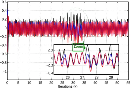
As shown in Figs. 4, 5 , for a small value ofλ(λ= 3), the state is very well estimated using the property of one sided-Lipschitz and also using the DMVT theorem. In the next part, the value ofλwill be increased to test the performance of the two observers. Consider nowλ= 500, with the same approach, we obtain :

0 5 10 15 20 25 30 35 40 45 50 55

−1 −0.8 −0.6 −0.4 −0.2 0 0.2 0.4 0.6

Iterations (k)

26 27 28 29

−0.4 −0.2 0 0.2

Zoom

Fig. 4: Response ofx2(k)(black line) and its estimates with O.S.L (red line) and DMVT (blue line)

0 5 10 15 20 25 30

−1.4 −1.2 −1 −0.8 −0.6 −0.4 −0.2 0 0.2 0.4 0.6

Iterations (k)

11 12 13 14 15 16 −0.6

[image:5.595.335.550.287.432.2]

−0.4 −0.2 0 0.2 0.4

Fig. 5: Response ofx3(k)(black line) and its estimates with O.S.L (red line) and DMVT (blue line)

L1=    

0.4610 0.01

−0.486 0.3662 0 −0.2006 0.0195 0.0462

   

;L2=    

0.9 0.01

−0.486 1.1077 0 0.6035 0.0195 8.6082    

(35)

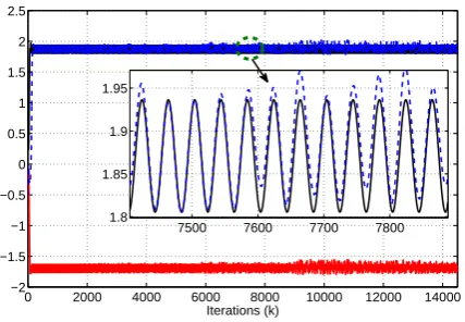
The state and its estimates are represented below in Fig. 6, keeping the same initial conditions given previously.

Remarks.

(1) it is remarkable that the estimated states by the DMVT-Observer, compared to those estimated by the One-sided-Observer, are more reliable especially with a very large Lip-schitz constant. The results given by O.S.O are biased (Fig 6).

[image:5.595.73.290.306.449.2]

0 2000 4000 6000 8000 10000 12000 14000 −2

−1.5 −1 −0.5 0 0.5 1 1.5 2 2.5

Iterations (k)

7500 7600 7700 7800 1.8

[image:6.595.74.288.75.223.2]

1.85 1.9 1.95

Fig. 6: Response ofx1(k)(black line) and its estimates with O.S.L (red line) and DMVT (blue line)

4. CONCLUSION

Efficient design of two observers for a class of nonlinear discrete systems are presented.

The two methods are then applied to real time state estimation of the one-link flexible joint robot using ARDUINO MEGA 2560 de-vice in two modes. The results have confirmed the high quality of estimation offered by the DMVT design method with: the presence of noises whose the amplitudes and frequencies are variable and with a large value of Lipschitz constant. The use of the DMVT had ensured a performed stability analysis with non restrictive sufficient condition based on LMI.

Acknowledgment

The authors would like to thank l’Institut Sup´erieur des Syst`emes Industriels de Gab`es and l’Institut Franc¸ais de Tunise for the real-ization of the practical tests.

5. REFERENCES

[1] Masoud Abbaszadeh and Horacio J. Marquez. Nonlinear ob-server design for one-sided lipschitz systems. InProc. Amer-ican Control Conf., pages 5284–5289, Marriott Waterfront, Baltimore, MD, USA, June 30-July 02, 2010.

[2] A. Alessandri. Design of observers for lipschitz nonlinear sys-tems using lmi. InNOLCOS, IFAC Symposium on Nonlinear Control Systems, Stuttgart, Germany, 2004.

[3] M. Benallouch, M. Boutayeb, and M. Zasadzinski. Observers design for one-sided lipschitz discrete-time systems. Syst. Control Letters, 61:879–886, 2012.

[4] M. Boutayeb. Identification of nonlinear systems in the pres-ence of unknown but bounded disturbances.IEEE Trans. on Autom. Control, 45:1503–1507, 2000.

[5] M. Boutayeb and C. Aubry. A strong tracking extended kalman observer for nonlinear discrete-time systems.IEEE Trans. on Autom. Control, 44:1550–1556, 1999.

[6] S. Boyd, L. El Ghaoui, E. Ferron, and V. Balakrishnan.Linear matrix inequalities in systems and control theory. Studies in Applied Mathematics SIAM, Philadelphia, 15 edition, 1994.

[7] Q.P. Ha and H. Trinh. State and input simultaneous estimation for a class of nonlinear systems.Automatica, 40:1779–1785, 2004.

[8] Pan Jinfeng, Meng Min, and Feng Jun-e. A note on observers design for one-sided lipschitz nonlinear systems. InControl Conference (CCC), 2015 34th Chinese, pages 1003–1007, July 2015.

[9] Linlin Li, Ying Yang, Yong Zhang, and S.X. Ding. Fault es-timation of one-sided lipschitz and quasi-one-sided lipschitz systems. InControl Conference (CCC), 2014 33rd Chinese, pages 2574–2579, July 2014.

[10] W. Lin and C. Byrnes. Remarks on linearization of discrete-time autonomous systems and nonlinear observer design. Syst. Control Letters, 25:31–40, 1995.

[11] P.R. Pagilla and Y. Zhu. Controller and observer design for lipschitz nonlinear systems. InProc. American Control Conf., pages 2379–2384, Boston, Massachusetts,USA, 2004. [12] R. Rajamani. Observer for lipschitz nonlinear systems.IEEE

Trans. on Autom. Control, 43:397–401, 1998.

[13] M. Spong. Modeling and control of elastic joint robots.Trans. ASME, J. Dyn. Syst., Meas. Control, 109:310–319, 1987. [14] A. Thabet, M. Boutayeb, and M. N. Abdelkrim. On the

mod-eling and state estimation for dynamic power system.Int. J. of Electronics Science and Engineering, 7 (2):181–190, 2013. [15] A. Thabet, M. Boutayeb, and M.N. Abdelkrim. Real time dy-namic state estimation for power system.Int J. of Computer Applications, 38-2:11–18, 2012.

[16] A. Thabet, G.B.H Frej, and M. Boutayeb. Observer-based feedback stabilization for lipschitz nonlinear systems with ex-tension toh∞performance analysis: Design and experimen-tal results.IEEE Trans. on Control Systems Technology, 26 (1):321–328, 2018.

[17] Chunyan Wang, Zongyu Zuo, Zongli Lin, and Zhengtao Ding. Consensus control of a class of lipschitz nonlinear systems with input delay. Circuits and Systems I: Regular Papers, IEEE Transactions on, 62(11):2730–2738, Nov 2015. [18] A. Zemouch and M. Boutayeb. A unifiedH∞ adaptive

ob-server synthesis method for a class of systems with both lipschitz and monotone nonlinearities.Syst. Control Letters, 58:282–288, 2009.

[19] A. Zemouch, M. Boutayeb, and G.I. Bara. Observers for a class of lipschitz systems with extension toH∞performance

analysis.Syst. Control Letters, 57:18–27, 2008.