Regionalization of River Basins Using Cluster Ensemble

Regionalization of River Basins Using Cluster Ensemble

Sangeeta Ahuja

Division of Computer Applications, IASRI (ICAR), New Delhi, India Email: [email protected], [email protected]

Received March 17, 2012; revised April 23, 2012; accepted May 26,2012

ABSTRACT

In the wake of global water scarcity, forecasting of water quantity and quality, regionalization of river basins has at-tracted serious attention of the hydrology researchers. It has become an important area of research to enhance the qual-ity of prediction of yield in river basins. In this paper, we analyzed the data of Godavari basin, and regionalize it using a cluster ensemble method. Cluster Ensemble methods are commonly used to enhance the quality of clustering by com-bining multiple clustering schemes to produce a more robust scheme delivering similar homogeneous basins. The goal is to identify, analyse and describe hydrologically similar catchments using cluster analysis. Clustering has been done using RCDA cluster ensemble algorithm, which is based on discriminant analysis. The algorithm takes H base cluster-ing schemes each with K clusters, obtained by any clustercluster-ing method, as input and constructs discriminant function for each one of them. Subsequently, all the data tuples are predicted using H discriminant functions for cluster membership. Tuples with consistent predictions are assigned to the clusters, while tuples with inconsistent predictions are analyzed further and either assigned to clusters or declared as noise. Clustering results of RCDA algorithm have been compared with Best of k-means and Clue cluster ensemble of R software using traditional clustering quality measures. Further, domain knowledge based comparison has also been performed. All the results are encouraging and indicate better re-gionalization of the Godavari basin data.

Keywords: K-Means; Cluster Ensemble; Hydrology; Runoff; Cultivation Area; Precipitation; Field Capacity

1. Introduction

Estimating design flow of ungauged basins is very cru- cial in the planning and management of hydraulic and water resources engineering. Regionalization for identi- fying homogeneous hydrologic regions is a well-accepted technique in this area. Regionalization is defined as de- termination of hydrologically similar units, and is one of the most challenging tasks in surface hydrology. In re- cent years several new mathematical and computational tools have been explored for this task [1].

Regionalization is done for estimating design flow in ungauged basins which is frequently encountered in the design and planning of hydraulic and water resources en- gineering [2]. The hydrologic regionalization technique is to infer required data in ungauged catchments from neighbour catchments where hydrologic data have been collected (e.g. Nathan and McMahon, 1990; Bullock and Andrews, 1997; Hall and Minns, 1999).

Runoff predictions in ungauged catchments are deter- mined by regionalization. Development of practical run- off prediction methods are important for assessing water resources in an ungauged or poorly gauged catchment which is usually located in headwater regions [2]. Excess runoff can lead to flooding, which occurs when there is too much precipitation.

Catchment shows a wide range of response behaviour, therefore, Regionalization is utilized for searching the hydrological similarity of catchments to characterize each catchment [3].

2. Background and Related Work

We present the related work with respect to two aspects

i.e. the techniques used for regionalization in hydrology studies and the techniques of cluster ensemble. Subse- quently we describe the discriminant based cluster en- semble algorithm (RCDA) used in this work.

2.1. Regionalization

Hydrological similarity of catchments is identified and analyzed in the paper [3] by using the concept of Self- Organizing Maps (SOM). SOM are plotted by utilizing the hierarchical clustering algorithm of cluster analysis.

A regional formula has been developed by the authors, using gauged flows and basin topographic characteristics in order to estimate the design flows in ungauged areas within the homogeneous region [1].

to the topographic variables at 5% significance level and the delineation of homogeneous regions can enhance the performance of regional formulae to estimate design flow.

Different regionalization methods were investigated in the paper [2], for modeling daily runoff in ungauged catchments for selecting donor catchments whose entire set of parameter values are used for target ungauged cat- chment by determine the spatial proximity, physical si- milarity and integrated similarity.

Regionalization of runoff formation by aggregation of hydrological response units for the representative ele- mentary areas (REAs), which are defined as homogene- ous, the hydrologically effective parameters can be clearly assigned. Aggregation approaches were used to analyse the research regions which differ in the composi- tion of their natural attributes. The purpose of the re- gional comparison is to reveal to what extent it is possi- ble to apply the regionalization strategy independent of the region and scale [4].

These analyses substantiate the fact that it is possible to achieve plausible results with the regionalization ap- proaches which have been developed, provided that geo- information for the entire region is available. The com- parison shows that the regionalization approaches are independent of area and scale and these regionalization procedures significantly improve the quality of simula- tion of the water balance for large drainage basins, with a significant reduction of the relational-geometric configu- rations [4].

2.2. Cluster Ensemble Approach

Motivation of Cluster Ensemble technique arises because of different clustering schemes that are obtained by ap- plication of different clustering algorithms, or by varying the parameters of the same clustering algorithm. For ex- ample, in k-means algorithm, which is one of the most used clustering algorithms, variations in results arise be- cause of the inherent randomization. Further, each algo- rithm performs differently depending upon the biases and assumptions associated with it.

Under such circumstances, it is very difficult to ascer- tain suitability of an algorithm for an application. Cluster ensemble techniques aims to improve the clustering sche- me by intelligently combining multiple schemes. This technique has caught attention of researchers in computer science community as it has found to substantially im- prove the robustness, stability, accuracy and quality of resulting clustering scheme [5-9]. An informative survey of various cluster ensemble techniques can be found in [5]. The problem of cluster ensemble is formally defined below.

Let D denote a data set of N, d-dimensional vectors Xi

= 1_, 2_, d

i Xi Xi

π

where i = 1, N, each representing an

object. D is subjected to a clustering algorithm which delivers a partition (i.e. a clustering scheme)  consi- sting of K clusters, i.e. (π = C1, C2, …, CK). Let λ' be

the function of π; (: -> {1,K}) that yields labeling for each of the N objects in D. Let





partitions of D obtained by applying either same cluster- ing algorithmon D or by applying H different clustering algorithms.

π ,π , , π



X

Before combining the schemes, it is necessary to es- tablish the correspondence between the clusters of dif- ferent schemes and relabel the corresponding clusters. Let {λ1, λ2, , λH} be the set of corresponding labeling

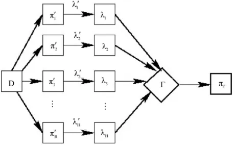
of H clustering schemes on D. The problem of cluster ensemble is to derive a consensus function Γ, which combines H partitions and delivers a clustering πf with a promise that πf is more robust than any of constituent H

partitions and best captures the natural structures in D.

Figure 1 shows the process of construction of cluster

ensemble.

It is the design of Γ that distinguishes different cluster ensemble algorithms to a large extent. Hyper graph parti- tioning [5] voting approach [10], mutual information [5, 11], co-associations [12-14] are some of the well-estab- lished approaches for building consensus functions.

2.3. RCDA (Robust Clustering Using Discriminant Analysis)

RCDA [15] is a recent algorithm for generating a robust clustering scheme using discriminant analysis. Robust Clustering Using Discriminant Analysis (RCDA) algo- rithm takes H partitions as input with K clusters in each partition and delivers a robust partition with same num- ber of clusters, and noise, if any. It operates in three phases. In the first phase clusters in each partition are relabeled to establish correspondence in H partitions. In the second phase the algorithm constructs a discriminant function for each partition, thereby resulting in H dis- criminant functions. Cluster label of each tuple in dataset

D is predicted by each of the H discriminant functions

resulting in N X H label matrix (L). This is a compute intensive phase of the algorithm and needs no user pa- rameter. Finally, in the third phase tuples with consistent labels are assigned to clusters in the final partition. Tu- ples with low consistency are refined and the leftover tuples are reported as noise. Different phases of RCDA algorithm is shown pictorially in Figure 2.

3. Regionalization Using RCDA

In this study the hydrological similarity of a catchment area has been investigated with respect to their response behaviour by using RCDA Algorithm. The goal is to identify, analyse and describe hydrologically similar catchments/regions by using the catchment characteris- tics such as Elevation, Precipitation, Aridity Index, Slope, Field Capacity and Stream Density.

Data from Godavari basin is processed using RCDA algorithm in order to regionalize the river basin. The data consists of 331 tuples and six attributes viz., Elevation, Precipitation, Aridity Index, Slope, Field Capacity and Stream Density respectively.

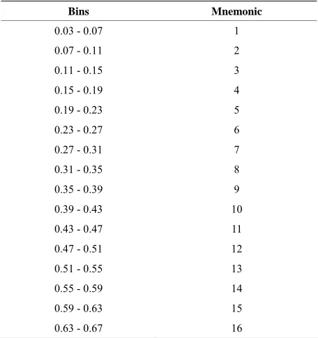
Since the numbers of regions are not known, the data is pre-processed using domain knowledge to estimate the number of clusters. Intuitively, the regions with same runoff/Catchment Area ratio should fall in same cluster. Based on this idea, runoff/Catchment Area ratio was computed for all tuples. The mnemonics for the bins for bin-widths (0.08 and 0.04) are represented in Table 1

and Table 2 respectively. The frequency charts for two

bin-widths (0.08 and 0.04) respectively were constructed as shown in Figure 3 and Figure 4.

It can be seen from the Figure 3 that last three bins

(numbered 6, 7 and 8 along x-axis) consists of only 0,1 and 2 tuples respectively. So, we eliminated the three noisy tuples and also it can be seen from the Figure 4

that last six bins (numbered (11, 12, 13, 15), 14, 16) con- sists of only 0, 1, 2 and 3 tuples respectively. So, we eliminated the six noisy tuples.

This analysis indicates that either there are five or nine regions in the Godavari basin. We applied RCDA algo- rithm to cluster 328 tuples after removing three noisy tuples in case of five regions and cluster 325 tuples after removing six noisy tuples in case of nine regions.

Figure 2. Three phases of RCDA algorithm.

Figure 3. Frequency Chart for runoff/Catchment Area ratio with bin width of 0.08.

Figure 4. Frequency Chart for runoff/Catchment Area ratio with bin width of 0.04.

Table 1. Description of data sets—mnemonics used for Bins.

Bins Mnemonic

0.03 - 0.11 1

0.11 - 0.19 2

0.19 - 0.27 3

0.27 - 0.35 4

0.35 - 0.43 5

0.43 - 0.51 6

0.51 - 0.59 7

0.59 - 0.67 8

4. Experimental Section

RCDA (Robust Clustering Using Discriminant Analysis) algorithm was implemented in Windowsenvironment as multi-threaded C++ program. R package (V 2.13.0) was used for statistical functions. Dual core Intel(R) machine (2.20 GHz, 4 GB RAM) was used for executing pro- grams. In this section we describe the goals and metho- dology of experiments.

Table 2. Description of data sets—mnemonics used for Bins.

Bins Mnemonic

0.03 - 0.07 1

0.07 - 0.11 2

0.11 - 0.15 3

0.15 - 0.19 4

0.19 - 0.23 5

0.23 - 0.27 6

0.27 - 0.31 7

0.31 - 0.35 8

0.35 - 0.39 9

0.39 - 0.43 10

0.43 - 0.47 11

0.47 - 0.51 12

0.51 - 0.55 13

0.55 - 0.59 14

0.59 - 0.63 15

0.63 - 0.67 16

rithm to get the clustering schemes. We describe the re- sults in two sections for the two possibilities.

Validation of results is performed both at computa- tional and domain level. Computational validation of re- sults is performed by comparing the SSE (Sum of Squ- ared Error) of the clustering scheme obtained by RCDA, with another cluster ensemble method available in R software and the best of the constituent clustering sche- me. The scheme with the lowest SSE is the best cluster- ing scheme (optimum partition). The domain level vali- dation is performed by comparing the purity and NMI of the obtained scheme with the frequency distribution shown in Figure 3 and Figure 5, which is taken as gold

standard. In subsequent sections, we detail the computa- tion of SSE and Purity.

4.1. Computing SSE

For measuring the quality of clustering, we use the Sum of Squared error (SSE), which is also known as scatter. In other words, we calculate the error of each data point,

i.e. its eucleidean distance to the closest centroid, and then compute the total sum of squared errors. If we have two different sets of clusters by two different algorithms (schemes), we prefer the one with the smallest squared error. The SSE [16]is formally defined as





i

dist x x

1

SSE

i

K

i x C



 

where dist is the standard Euclidean distance between the two objects in eucleidean space, Ci = ith cluster, x is a

point in Ci and xi is the mean (centroid) of the i

th _clus-

Figure 5. Comparison of SSE of RCDA, Clue and Best of K-means (Km) algorithm for K = 5.

ter1_.

4.2. Computing Purity

For each cluster, the class distribution of the data is cal-culated first, i.e. for cluster j we compute pij, the

prob-ability that a member of cluster i belongs to belong j as

pij = mij/mi, where mi is the number of objects in cluster i

and mij is the number of objects of class j in cluster i.

The purity of cluster i is defined in [16] as

 

max ij

i _j p

p  (2)

The overall purity of a partition is

1 Purity K i

i i

m p m







In general, larger value of purity indicates better quality of the solution.

4.3. Computing NMI (Normalized Mutual Information)

Intuitively, the optimal combined clustering should share the most information with the original clusterings. Thus NMI has been used by researchers to measure cluster quality [11].

Let A and B be the random variables described by the cluster labeling λ(a) and λ(b) with k(a) and k(b) groups respectively. Let I(A,B) denote the mutual information between A and B, H(A), H(B) denote the entropy of A and B respectively. Then normalized mutual information (NMI) is defined as follows

NMI(A,B) = 2 I(A,B)/(H(A) + H(B)) (4) Clearly, the value lies between [0, 1] and NMI(A,A) = 1.

Equation (4) is estimated by the sampled entities pro-vided by the clustering. Let n(h) _{be the number of objects}

in cluster ch according to λ(a) and let ng be the number of

objects in cluster cg according to λ(b). Let nhg be the

1_{Here, in our case xis the tuple consists of six attributes (catchment}

number of objects in cluster ch according to λ(a) as well

as in cluster cg according to λ(b). The normalized mutual

information criteria φ(NMI) is computed as follows

   

 

 

   

 

, 1 1

2

log

ka kb

NMI h

g

h g

a b _n n

 

 _{ } gh

kakb h g

n n n n

  

 _

 

  (5)

In our context, k(a) = k(b) = k.

4.4. Results with 5 Clusters

We experimented the dataset with RCDA cluster ensem- ble algorithm [15] for K (number of clusters = 5) with varying the number of partitions (H = 2, 4, 6, 8, 10, 12, 14, 16 and 18) respectively. Here, we get the optimum partition H = 8, because at this value of partition, we ob- tained the lowest value of SSE (Sum of Squared Error)

and maximum (improved) clustering quality. The com- parison of the RCDA algorithm with Best of K-means (Km) and Clue Ensemble obtained from R software [17] have been done by determining the centroids as shown in

Table 3 and Total SSE (Sum of Squared Error) of each

algorithm as shown in Figure 5. Moreover, comparisons

of RCDA algorithm with Best of K-means (Km) and Clue Ensembleobtained from R software [17] have been done in terms of measuring Purity and NMI (Normalized Mutual Information) as shown in Figure 6.

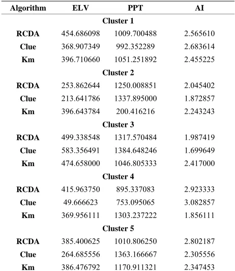
Table 3 shows the centroids of each cluster of RCDA

and Clue algorithm for K = 5 number of clusters. ELV, PPT, AI, Sl, FC and SD in Table 3 represents the Eleva-

tion, Precipitation, Aridity Index, Slope, Field Capacity and Stream Density respectively.

4.5. Results with 9 Clusters

Similarly, we experimented the dataset with RCDA clus-ter ensemble algorithm [15] for K (number of clusclus-ters = 9) with varying the number of partitions (H = 2, 4, 6, 8, 10, 12, 14, 16 and 18) respectively. Here, we get the op-timum partition H = 8, because at this value of partition, we obtained the lowest value of SSE (Sum of Squared Error) and maximum (improved) clustering quality.

The comparison of the RCDA algorithm with Best of K-means (Km) and Clue Ensemble obtained from R soft- ware [17] have been done by determining the centroids as shown in Table 4 and total SSE of the each algorithm

as shown in Figure 7. Moreover, comparisons of RCDA

algorithm with Best of K-means (Km) and Clue Ensem- ble obtained from R software [17] have been done in terms of measuring Purity and NMI (Normalized Mutual Information) as shown in Figure 8.

5. Discussion of Results

We observed from the Figure 5 and Figure 7 that total

SSE of RCDA algorithm is less than as compared to the

Figure 6. Comparison of purity and NMI of RCDA, Clue and Best of K-means (Km) algorithm for K = 5. \label {Fig_PN5}.

Figure 7. Comparison of SSE of RCDA and Clue algorithm for K = 9.

Figure 8. Comparison of purity and NMI of RCDA, Clue and Best of K-means (Km) algorithm for K = 9.

total SSE of Clue Algorithm which clearly describes that variability reduces in case of RCDA algorithm as com- pared to clue algorithm which is the characteristics of good quality clustering.

Moreover, the Purity and NMI of RCDA algorithm improves as compared to Best of K-means (Km) and Clue cluster Ensemble obtained from R software as shown in

Figure 6 and Figure 8.

Finally, from the above it is concluded that K = 9 with H

Table 3. Centroids of each cluster for RCDA, Clue and Best of K-means (Km) algorithm for K = 5.

Algorithm ELV PPT AI

Cluster 1

RCDA 454.686098 1009.700488 2.565610 Clue 368.907349 992.352289 2.683614

Km 396.710660 1051.251892 2.455225

Cluster 2

RCDA 253.862644 1250.008851 2.045402 Clue 213.641786 1337.895000 1.872857

Km 396.643784 200.416216 2.243243

Cluster 3

RCDA 499.338548 1317.570484 1.987419 Clue 583.356491 1384.648246 1.699649

Km 474.658000 1046.805333 2.417000

Cluster 4

RCDA 415.963750 895.337083 2.923333 Clue 49.666623 753.095065 3.082857

Km 369.956111 1303.237222 1.856111

Cluster 5

RCDA 385.400625 1010.806250 2.802187 Clue 264.685556 1363.166667 2.305556

Km 386.476792 1170.911321 2.347453

Table 4. Centroids of each cluster for RCDA, Clue and Best of K-means (Km) algorithm for K = 9.

Algorithm ELV PPT AI

Cluster 1

RCDA 304.728148 1251.386667 2.077407 Clue 568.021707 1367.127073 1.738049

Km 528.729299 801.104068 2.666991

Cluster 2

RCDA 551.496296 834.513889 2.880556 Clue 597.165897 825.544615 2.799231

Km 324.264769 1265.239846 2.049538

Cluster 3

RCDA 316.341481 1000.493333 2.691111 Clue 274.213509 1093.276491 2.508772

Km 340.568000 1360.779143 1.784286

Cluster 4

RCDA 462.077500 922.229583 2.862708 Clue 253.567727 1398.051591 1.763409

Km 450.545429 808.076286 3.167714

Cluster 5

RCDA 236.166197 1297.978310 1.970845 Clue 503.114103 686.310256 3.327949

Km 420.485789 782.421053 3.460000

Cluster 6

RCDA 565.201000 814.138000 2.709000 Clue 711.091818 1375.290000 1.617273

Km 295.265294 1331.299412 1.807647

Continued

Cluster 7

RCDA 759.509375 1237.728125 1.816250

Clue 181.243784 1262.656486 1.998649

Km 481.933000 940.910500 2.678000

Cluster 8

RCDA 473.920000 1597.883810 1.528571 Clue 391.232727 1784.505455 1.730909

Km 671.832353 1312.657647 1.675294

Cluster 9

RCDA 382.813333 1079.631667 2.767500

Clue 409.789348 938.381739 2.843696

Km 223.790179 1234.093929 2.076786

Algorithm Sl FC SD

Cluster 1

RCDA 0.019019 15 0.370370 0.103417 Clue 0.031683 17 7.814634 0.071464

Km 0.016468 14 5.872376 0.103357

Cluster 2

RCDA 0.015907 152.312963 0.110959 Clue 0.018077 189.923077 0.095857

Km 0.021815 151.692308 0.102434

Cluster 3

RCDA 0.013370 261.585185 0.024368 Clue 0.017737 179.547368 0.056450

Km 0.026857 156.571429 0.096325

Cluster 4

RCDA 0.013375 155.39375 0 0.014827 Clue 0.024159 154.565909 0.045808

Km 0.013571 147.714286 0.013118

Cluster 5

RCDA 0.018718 144.225352 0.009158 Clue 0.012051 150.769231 0.071786

Km 0.015737 142.105263 0.014265

Cluster 6

RCDA 0.019100 312.000000 0.174771

Clue 0.046545 177.21818 0.095623

Km 0.035353 174.705882 0.010749

Cluster 7

RCDA 0.046688 178.993750 0.107478 Clue 0.018703 145.945946 0.033421

Km 0.018950 283.905000 0.142880

Cluster 8

RCDA 0.058810 160.952381 0.061680

Clue 0.028091 154.545455 0.062202

Km 0.067765 183.182353 0.083542

Cluster 9

RCDA 0.015667 236.850000 0.102557 Clue 0.015348 206.369565 0.068397

in Figure 5 and Figure 7. Similarly, the Purity and NMI

of RCDA algorithm for both the cases K = 5 and K = 9 is more as compared to Clue and Best of K-means (Km) algorithm, but it improves much more in case of K = 9 which indicates that more homogeneous catchments are clustered using RCDA algorithm with K = 9 number of clusters.

6. Acknowledgements

Expressing my sincere thanks to Dr. Vasudha Bhatnagar, Head, University of Delhi, Delhi, India and Dr. Subhash Chander, Professor (Retd.) of Water Resources, Civil Engineering Department, IIT Delhi, India for their help and encouragement for the production of this manuscript.

REFERENCES

[1] P.-S. Yu, H.-P. Tsai, S.-T. Chen and Y.-C. Wang, “Esti-mation of Design Flow in Ungauged Basins by Region-alization,” Department of Hydraulic and Ocean Engi-neering, National Cheng Kung University, Taiwan, 2005. [2] Y. Zhang and F. Chiew, “Evaluation of Regionalization

Methods for Predicting Runoff in Ungauged Catchments in Southeast Australia,” CSIRO Water for a Healthy Country National Research Flagship, CSIRO Land and Water 13-1, 2009.

[3] R. Ley, M. C. Casper, H. Hellebrand and R. Merz, “Catchment Classification by Runoff Behaviour with Self-Organizing Maps (SOM),” Journal of Hydrology and Earth System Sciences, Vol. 15, 2011, pp. 2947- 2962. doi:10.5194/hess-15-2947-2011

[4] G. Busch, J. Sutmoller and G. Gerold, “Regionalization of Runoff Information by Aggregation of Hydrological Response Units: A Regional Comparison,” Proceedings of a Conference Regionalization in Hydrology, Vol. 254, 1997.

[5] R. Ghaemi, N. Sulaiman, H. Irahim and N. Mustapha, “A Survey: Clustering Ensembles Techniques,” Proceedings of World Academy of Science, Engineering and Technol-ogy, Vol. 38, No. 2, 2002, pp. 2070-3740.

[6] X. Hu and I. Yoo, “Cluster Ensemble and Its Applications in Gene Expression Analysis,” Proceedings of Second

Asia-Pacific Bioinformatics Conference, Vol. 29, 2004, pp. 297-302.

[7] A. Topchy, B. Minaei-Bidgoli, A. K. Jain and W. F. Punch, “Adaptive Clustering Ensembles,” Proceedings of the 17th International Conference on Pattern Recognition, Vol. 1, 2004, pp. 272-275.

doi:10.1109/ICPR.2004.1334105

[8] A. Topchy, A. K. Jain and W. Punch, “A Mixture Model for Clustering Ensembles,” Proceedings SIAM Confer-ence on Data Mining, 2004, pp. 379-390.

[9] M. D. Frossyniotis and A. Stafylopatis, “A Multi-Clus-tering Fusion Algorithm,” SETN’02 Proceedings of the Second Hellenic Conference on AI: Methods and Applica-tions of Artificial Intelligence, Springer, London, 2002. [10] B. Fischer and J. M. Buhmann, “Path-Based Clustering

for Grouping of Smooth Curves and Texture Segmenta-tion,” IEEE Transaction on Pattern Analysis and Ma-chine Intelligence, Vol. 25, No. 4, 2003, pp. 513-518. doi:10.1109/tpami.2003.1190577

[11] A. Strehl and J. Ghosh, “Cluster Ensembles—A Knowl-edge Reuse Framework for Combining Multiple Parti-tions,” Journal of Machine Learning Research, Vol. 3, 2002, pp. 583-617.

[12] A. L. N. Fred, “Finding Consistent Cluster in Data Parti-tions,” Proceedings of 2nd International Workshop on Multiple Classifier Systems, Vol. 2096, 2001, pp. 309- 318.

[13] A. L. N. Fred and A. K. Jain, “Data Clustering Using Evidence Accumulation,” Proceedings of International Conference on Pattern Recognition, Vol. 4, 2002, pp. 276-280.

[14] A. Topchy, A. K. Jain and W. Punch, “Combining Multi-ple Weak Clusterings,” Proceedings of the 3rd IEEE In-ternational Conference on Data Mining, 19-22 November 2003, pp. 331-338. doi:10.1109/ICDM.2003.1250937 [15] V. Bhatnagar and S. Ahuja, “Robust Clustering Using

Discriminant Analysis,” Proceedings of International In-dustrial Conference on Data Mining, Vol. 6171, 2010, pp. 143-157.

[16] P. N. Tan, V. Kumar and M. Steinbach, “Introduction to Data Mining,” Pearson, March 2006.