A New Test for Unknown Age Class of Life Distribution
based on Laplace Transform Technique
S. E. Abu-Youssef
Department of Mathematics,
Faculty of Science,
Al-Azhar University, Cairo,
Egypt
Nahd S. A. Ali
Department of Mathematics,
Faculty of Education,
Ain Shams University, Cairo,
Egypt
M. E. Bakr
Egyptian General Authority for
Meteorology, Ministry of Civil
Aviation, Cairo, Egypt
ABSTRACT
Most of the approaches suggested during the last decades for solving life testing problems are markedly different from those used in the related but wider area of Laplace transform technique. In this paper, it is demonstrated that applying the Laplace transform technique makes sense also for solving life testing problems and that result in simpler procedures that are asymptotically equivalent or better than standard ones. A new test statistics for testing exponentiality against used better than age in the Laplace transform order aging class of life distribution (UBAL) is proposed. Pitman’s asymptotic efficiencies of this test are calculated and compared with other tests. The percentiles of this test statistic are tabulated for censored and non-censored data. Finally, examples in different areas are used as practical applications of the proposed test.
Keywords
UBA and UBAL classes of life distributions; Testing hypothesis; Right censored data; Makeham, Weibull, Linear failure rate (LFR) distributions.
1.
INTRODUCTION
Statistical inferences are used to project the data from the sample to the entire population. Statistical inference based on two main branches one of them the estimation and the other is testing hypotheses. In general, we do not know the true value (claim) of population parameters they must be estimated. However, we do have hypotheses about what the true values (claims) are. The hypothesis actually to be tested is usually given the symbol H0, and is commonly referred to as the null
hypothesis. The other hypothesis, which is assumed to be true when the null hypothesis is false, is referred to as the alternative hypothesis, and is often symbolized H1. Both the
null and alternative hypothesis should be stated before any statistical test of significance is conducted.
In the last decade, various classes of life distributions have been proposed in order to model different aspects of aging. We get the well-known classes of increasing failure rate (IFR), increasing failure rate on average (IFRA), and used better than aged (UBA), used better than aged in expectation (UBAE). Properties and applications of these aging notions can be found, for instance, in Bryson and Siddiqui (1969), Barlow and Proschan (1981), Ahmad (2004).
In this paper, we interest in the used better than aged in Laplace transform order aging class of life distribution UBAL which introduced by Abu-Youssef and Bakr (2018).
A real data is given and we desire to test H0: data is
exponential versus the alternative hypothesis H1: data is not
exponential. To choose between H0 and H1 or to make a
decision we need to define test statistic. The test statistic is a
random variable used to determine how close a specific sample result falls to one of the hypotheses being tested. In reliability theory, aging life is usually characterized by a nonnegative continuous random variable X ≥ 0 representing equipment life with distribution function F and survival function F t = 1 − F(t) such that F 0 − = 0. One of the most important approaches to the study of aging is based on the concept of the residual life. For any random variable X, let Xt= X − t X > 𝑡 , t ∈ x: F x < 1 , denote a random
variable whose distribution is the same as the conditional distribution of X − t given that X > 𝑡 and has survival function
F t x = F (x+t)
F
(t) F t > 0
0 F t = 0 .
When X is the lifetime of a device which has a finite mean μ= E X = F u du0∞ , the mean of Xt is
called mean residual life (MRL) and is given by μ t = E Xt =
Ft∞ u du F t .
Further, the hazard rate of X is defined by h t = −d
dtln F t = f t
F t , t ≥ 0, F t > 0,
where f(t) = F′(t) is the probability density of X assuming it exist. Note that if limt→∞h(t) = h(∞) it exists and is positive,
then (Willmot and Cai (2000)) μ∞ = limt→∞μ(t) =h(1∞).
We review some common notions of stochastic orderings and aging notions are considered in this paper (see Barlow and Proschan (1981)).
If X and Y are two random variables with distributions F and G (survivals F and G), respectively, then we say that X is smaller than Y in the:
a) Usual stochastic order, denoted by X ≤st Y if
F (x) ≤ G (x) for all x.
b) Increasing convex order, denoted by X ≤icx Y if
F (u)
∞
x
du ≤ G∞ u
x
du.
c) Increasing concave order, denoted by X ≤icv Y if
F (u)
x 0
du ≤ Gx u
0
Another important ordering that has come to use in reliability and life testing is the following:
A random variable X is smaller than a random variable Y with respect to Laplace transform order (denoted by X ≤Lt Y ) if,
and only, if
e∞ −sxdF(x) 0
≥ e∞ −sxdG x 0
, s ≥ 0 (1.1)
It is easy to check that (1.1) is equivalent to e−sxF (x)
∞
0
dx ≤ e−sxG x
∞
0
dx (1.2)
Two classes of life distributions were introduced by Alzaid (1994) which are used better than aged (UBA) and used better than aged in expectation (UBAE) classes of life distribution. Precisely we have the following
definitions:
Definition (1.1): The df F is said to be used better than aged (UBA) if 0 < 𝜇 ∞ <∞ and for all x, t ≥ 0, (See Ahmad (2004))
F x + t ≥ F t e−x/μ(∞), x, t ≥ 0 (1.3)
Definition (1.2): The distribution function
F
is said to be used better than aged in expectation (UBAE) if 0 < 𝜇 ∞ < ∞ and for all x, t ≥ 0,μ t ≥μ ∞ (1.4) Note that, F is UBA (UBAE) if and only if Xt converges in
distribution to a random variable XA (say) exponentially
distributed with failure rate 1μ and
𝑿𝒕 ≤𝒔𝒕𝑿𝑨, 𝑬 𝑿𝒕 ≤𝒔𝒕𝑬 𝑿𝑨 .
According to the above definitions (1.1), (1.2) and (1.3) we can deduce the following new definition for used better than aged in the Laplace transform order as follows.
Definition (1.3): The distribution function F is said to be used better than aged in the Laplace transform order (UBAL) if 0 < 𝜇 ∞ <∞ and for all x, t ≥ 0,
e−sxF (x + t)
∞
0
dx ≥ μ ∞
1 + sμ ∞ F t , s ≥ 0 (1.5)
It is obvious that (1.3) is equivalent to 𝑿𝒕 ≤𝑳𝒕𝑿𝑨 for all t ≥
0.
To introduce the definition of the discrete UBAL, let X be a discrete non-negative random variable such that
P X = k = pk, k = 0, 1, 2, . .. . Let
P𝒌= 𝑷 𝑿 > 𝑘 , 𝒌 ≥ 𝟏, P0=1 denote the corresponding survival function.
The discrete non-negative random variable X is said to be discrete used better than aged in Laplace transform order (discrete UBAL) if, and only, if
P𝑘+𝑖𝑧𝑘 ≥
∞
𝒌=𝟎 P𝑖 ∞𝒌=𝟎𝑧𝑘, 𝒇𝒐𝒓 𝒂𝒍𝒍 𝟎 ≤ 𝒛 ≤ 𝟏 𝒂𝒏𝒅 𝒊 =
𝟎, 𝟏, … .
Now,
𝑿 ≤𝒔𝒕 𝑿𝑨 ⇒ 𝑿 ≤𝑳𝒕 𝑿𝑨.
Then, we have the following implication: (Abu-Youssef and Bakr (2014, 2018) and Abu-Youssef et al (2015, 2017)).
IFR
UBA
UBAL
UBAE
Applications, properties and interpretations of the Laplace transform order in the statistical theory of reliability, and in economics can be found in Denuit (2001), Klefsjo (1998) and Ahmed and Kayid (2004).
The main object in this paper is to deal with the problem of testing H0∶ F is exponential against H1∶ F is the largest class
of life distribution UBAL. The paper is organized as follows: in section 2, we give a test statistic based on Laplace Transform technique for complete data. Selected critical values are tabulated for sample sizes 5(5)100 is investigated using mathematica 8 programme in section 3. The Pitman asymptotic efficiency for common alternatives is obtained in section 4. In section 5; a proposed test is presented for right censored data. Finally, we discuss some applications (numerical examples) to show the importance of the proposed test in section 6.
2.
TESTING FOR COMPLETE DATA
This section is concerned with the construction of the proposed statistic as a Laplace Transform technique and discussing its asymptotic normality.
Here, we hope to test the null hypothesis 𝐻0∶ 𝐹 is
exponential, against 𝐻1∶ 𝐹 is UBAL, and is not
exponential. Non-parametric testing for classes of life distributions has been considered by many authors (see Mahmoud and Abdul Alim (2008); Abu-Youssef and Bakr (2014, 2018); Abu-Youssef et al (2015)).
According to Eq. (1.5) we may use the following as a measure of departure from 𝐻0.
δ𝐿 s,β = 𝑒−𝛽𝑡𝑒−𝑠𝑥F 𝑥 + 𝑡
∞
0
d𝑥 ∞
0
− 𝜇(∞) 1 + 𝑠𝜇(∞)𝑒
−𝛽𝑡𝐹 𝑡 d𝑡
= 𝑒−𝛽𝑡𝑒−𝑠𝑥F 𝑥 + 𝑡 𝑑𝑥𝑑𝑡
∞
0
− 𝜇(∞) 1 + 𝑠𝜇(∞) e
−βtF t 𝑑𝑡
∞
0
∞
0
.
The following theorem is essential for the development of our test statistic.
Theorem 4: Let X be the UBAL random variable with distribution function F; then based on the previous technique, δ𝐿 s,β =
1
𝑠 β− s 1 − φ s
− 1 + 𝛽 + 𝑠 1 − 𝜇 ∞
β β− s 1 + s𝜇 ∞ 1 − φβ (2.1)
Whereφ s = e∞ −sxdF(x) 0 .
δ𝐿 s,β = 𝑒−𝛽𝑡e−suF u + t
∞
0
dudt
∞
0
− 𝜇(∞) 1 + 𝑠𝜇(∞) 𝑒
−𝛽𝑡F 𝑡
∞
0
d𝑡.
= 𝐼 − 𝜇(∞) 1 + 𝑠𝜇(∞)𝐼𝐼. Where,
𝐼 = 𝑒−𝛽𝑡e−suF u + t
∞
0
dudt
∞
0
= 𝑒∞ −𝛽𝑡e−s(x−t)F x t
dxdt
∞
0
= 1 𝛽 − 𝑠 𝑒
−𝑠𝑡(1 − e−(β−s)t)F t dt
∞
0
= 1 𝛽 − 𝑠
1
s 1 −φ s − 1
β 1 −φ β . And
𝐼𝐼 = 𝑒∞ −𝛽𝑡F 𝑡 0
d𝑡
=1
𝛽 1 −φβ . Hence, the result follows.
Let 𝑋1, 𝑋2, … , 𝑋𝑛be a random sample from the distribution
function F.
For generality, we assume 𝜇(∞) is known and equal one. The empirical estimator
δ
s,β of our test statistic can be obtained as follows: δ𝐿𝑛 s,β = 1
𝑛(𝛽 − 𝑠) 1 𝑠 1 − e
−sXi
i
−ββ+ 1 (1 + s) 1 − e
−βXi .
To make the test is invariant, let ∆ 𝐿𝑛 s,β =δ𝐿𝑛 s,β
X .
Let us rewrite δ𝐿 as follows,
∆ 𝐿𝑛 s,β = 1 X
𝑛 ∅(Xi) i
where ∅ Xi =
1 𝛽 − 𝑠
1 𝑠 1 − e
−sXi − β+ 1
β(1 + s) 1 − e
−βXi .
To find the limiting distribution of δ (s,β) we resort to the U-statistic theory and practice (Lee (1990)).
Set ∅ X1 =
1 𝛽 − 𝑠
1 𝑠 1 − e
−sX1 − β+ 1
β(1 + s) 1 − e
−βX1 .
Then, ∆ 𝐿𝑛 s,β is equivalent to U-statistic given by: 𝑈𝑛=
1
𝑛 1
∅(Xi) i
.
The following theorem summarizes the asymptotic normality of δ𝐿 𝑛 s,β .
Theorem 5.
i- As n →∞, (δ𝐿𝑛 s,β −δ𝐿(s,β)) is asymptotically
normal with mean 0 and variance σ2 s,β where, σ2 s,β = Var δ
𝑛 s,β =
= E 1 𝛽 − 𝑠
1 𝑠 1 − e
−sXi
−ββ+ 1 (1 + s) 1 − e
−βXi
2
ii- Under 𝐻0, the variance is given by
σ02 s,β = 2
(2b + 1)(2𝑠 + 1) 𝑠 + 1 2(𝑠 + 𝑏 + 1).
Proof:
i- Using standard U-statistic theory, Lee (1990) and direct calculations, we get 𝐸 δ𝑛 s,β = 𝐸
1 𝛽 − 𝑠
1 𝑠 1 − e
−sXi
−ββ+ 1 (1 + s) 1 − e
−βXi ;
σ2 s,β = Var δ
𝑛 s,β =
= E 1 𝛽 − 𝑠
1 𝑠 1 − e
−sXi
− β+ 1 β(1 + s) 1 − e
−βXi
2
.
ii- Under 𝐻0, the parameter 𝑠 = 0.6,
𝛽 = 0.1 say, and
𝜇0= 𝐸 δ𝑛 s = 0;
σ02 0.6, 0.1 = 2
(2b + 1)(2𝑠 + 1) 𝑠 + 1 2(𝑠 + 𝑏 + 1)
= 0.17.
3.
MONTE CARLO NULL
DISTRIBUTION CRITICAL POINTS
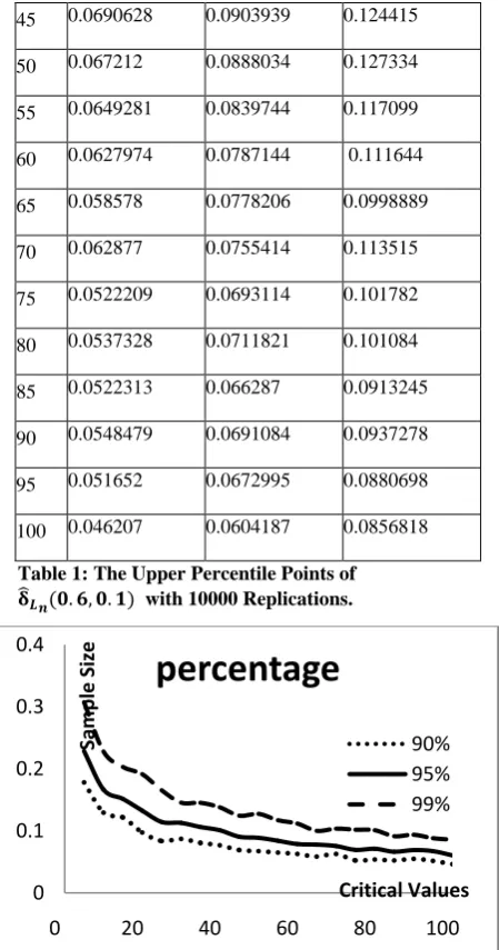
Based on 10000 generated samples from the standard exponential distribution the Monte Carlo null distribution critical values of our test δ𝐿𝑛(0.6, 0.1) are simulated and tabulated, where n = 5(5)100 in Table 1. Mathematica 8 programme is used.n 90% 95% 99%
5 0.178107 0.22842 0.307209
45 0.0690628 0.0903939 0.124415 50 0.067212 0.0888034 0.127334 55 0.0649281 0.0839744 0.117099 60 0.0627974 0.0787144 0.111644 65 0.058578 0.0778206 0.0998889 70 0.062877 0.0755414 0.113515 75 0.0522209 0.0693114 0.101782 80 0.0537328 0.0711821 0.101084 85 0.0522313 0.066287 0.0913245 90 0.0548479 0.0691084 0.0937278 95 0.051652 0.0672995 0.0880698 100 0.046207 0.0604187 0.0856818
[image:4.595.308.538.255.717.2]Table 1: The Upper Percentile Points of 𝛅𝑳𝒏(𝟎. 𝟔, 𝟎. 𝟏) with 10000 Replications.
Fig. 1: The Relation Between Sample Size and Critical Values.
From Table 1 and Fig. 1, the critical values decrease as the sample size increases and they increase as the confidence level increases.
4.
PITTMAN ASYMPTOTIC RELATIVE
EFFICIENCY
Since the above test statistic ∆ 𝐿 s,β =
δ𝐿
X is new and no other
tests are known for this class (UBAL). We may compare our test to the other classes. Here we choose the test ∆θ,(1)
presented by Mugdadi and Ahmad (2005) and δF(2)n presented Mahmoud and Abdul Alim (2008) for (NBAFR) class of life distribution. Then comparisons are achieved by using Pitman asymptotic relative efficiency PARE, which is defined as follows:
Let T1n and T2n be two statistics, then PARE of T1n relative
to T2n is defined by
e T1n, T2n =
μ1\ θ0
σ1 θ0
μ2\(θ0)
σ2(θ0).
Where μi\θ0 = limn→∞∂∂θE(Tni) θ
→θ0
, and σi2 θ
0 = limn→∞var(Tni).
Three of the most commonly used alternatives they are: (i) Linear failure rate family
F 1 x = e−x− x2
2θ, θ, x ≥ 0. (4.1)
(ii) Weibull family: F 2 x = e−x
θ
, θ≥ 1, , x ≥ 0. (4.2) (iii) Makeham family:
F 2 x = e−x−θ(x+e
−x−1)
, θ, x ≥ 0. (4.3) Note that H0(the exponential distribution) is attained at θ= 0
in (i), (iii) and θ= 1 in (ii). The Pitman's asymptotic efficiency (PAE) of δ𝐿 s,β is equal to
PAE δ𝐿 s,β =
∂
∂θ δ𝐿 s,β
θ→θ0
σ0 s,β
=
= 1
σ0 s,β
1 s(β− s) e
−sxdF
θ0
\
x
∞
0
− β+ 1
𝛽(1 + 𝑠)(𝛽 − 𝑠) e
−βxdF
θ0
\
x
∞
0
Where Fθ0
\
x = d
dθFθ(u) θ→θ0
This leads to:
(i) PAE in case of the linear failure rate distribution:
PAE δ𝐿 0.6, 0.1 = 1 σ0 0.6, 0.1
−1 0.3 e
−0.6xd −x2
2e
−x
∞
0
−−1.1 0.08 e
−0.1x
∞
0
d(−x
2
2 e
−x) = 1.77
(ii) PAE in case of the Weibull distibution:
PAE δ𝐿 0.6, 0.1 =
=σ 1
0 0.6, 0.1
−1 0.3 e
−0.6xd(−xln x e−x)
∞
0
−−1.1 0.08 e
−0.1xd(−xln x e−x)
∞
0
= 0.98
(iii) PAE in case of the Makeham distribution.
PAE δ 0.6, 0.1 = 1 σ0
−1 0.3 e
−0.6xd( 1 − x − e−x e−x)
∞
0
−−1.1 0.08 e
−0.1x
∞
0
d( 1 − x − e−x e−x)
= 0.58
Direct calculations of PAE of ∆θ,(1) , δFn
(2)
and δ𝐿 s,β are
summarized in table (2), the efficiencies in table shows clearly our test δ𝐿 s,β perform well for F1, F2 and F3.
0
0.1
0.2
0.3
0.4
0
20
40
60
80
100
Sample
Size
Critical Values
percentage
Distribution ∆θ,(1) δFn
(2) δ 𝐿 s,β
LFR 0.408 0.217 1.77
Weibull 0.170 0.050 0.98
[image:5.595.62.273.72.154.2]Makeham 0.0395 0.144 0.58
Table 2: PAE of ∆𝛉,(𝟏) , 𝛅𝐅𝐧
(𝟐)
and 𝛅𝑳 𝐬, 𝛃
In table (3), we give PARE's of δ𝐿 s,β with respect to ∆θ,(1)
and δF(2)n whose PAE are mentioned in table 2.
Distribution e(δ𝐿 s,β , ∆θ,(1)) e δ𝐿 s,β ,δFn
(2)
LFR 4.3 7.8
Weibull 5.76 19.6
[image:5.595.313.534.74.793.2]Makeham 14.68 4.03
Table 3: PARE of 𝛅𝑳 𝐬, 𝛃 with respect to ∆𝛉,(𝟏) and 𝛅𝐅𝐧
(𝟐)
.
It is clear from table (3) that the statistic δ𝐿 s,β perform well for F 1, F 2 and F 3 and it is more efficient than both ∆θ,(1) and
δF(2)n for all cases mentioned above. Hence our test, which deals the much larger UBA is better and also simpler.
5.
TESTING FOR RIGHT CENSORED
DATA
In this section, a test statistic is proposed to test: H0 (F is
exponential distribution with mean μ) versus H1 (F is UBAL
and not exponential distribution); with randomly right-censored data.
It is known that a censored data is usually the only information available in a life testing model or in a clinical study where patients may be lost (censored) before the completion of a study. We can describe the experimental situation as follows. Suppose n units are put on test, and X1, X2, … , Xn denote their true life time. Let that
X1, X2, … , Xnbe independent and identically distributed (i.i.d.)
according to a continuous life distribution F.
Let Y1, Y2, … , Yn be (i.i.d.) according to a continuous life
distribution G. Also we assume
that X,s and Y,s are independent. In the randomly right censored model, we observe the pairs
(Zi,δi), 𝑖 = 1, … , 𝑛 where Zi= min(Xi, Yi) and we assume
𝜇 ∞ is known and equal one. and δi=
1 if Zi= Xi (i th observation is uncensored)
0 if Zi= Yi i th observation is censored .
Let Z(0)< Z 1 < … < Z(n) denoted the ordered of Z’s and
δi is the δ corresponding to Z(i), respectively. Using the
Kaplan and Meier estimator in the case of censored data (Zi,δi), i = 1, … , n as follows:
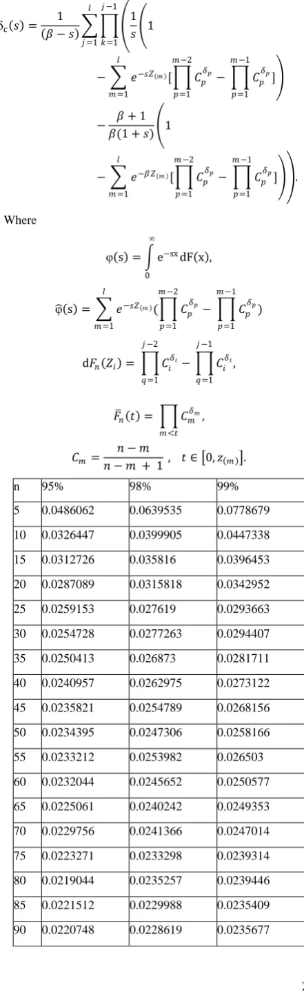
δc 𝑠 =
1
𝛽 − 𝑠 1 𝑠 1
𝑗 −1
𝑘=1 𝑙
𝑗 =1
− 𝑒−𝑠𝑍 𝑚 [ 𝐶
𝑝 𝛿𝑝
−
𝑚 −2
𝑝=1
𝐶𝑝𝛿𝑝
𝑚 −1
𝑝=1
]
𝑙
𝑚 =1
− 𝛽 + 1 𝛽(1 + 𝑠) 1
− 𝑒−𝛽 𝑍 𝑚 [ 𝐶
𝑝 𝛿𝑝
−
𝑚 −2
𝑝=1
𝐶𝑝𝛿𝑝
𝑚 −1
𝑝=1
]
𝑙
𝑚 =1
.
Where
φ s = e−sxdF x
∞
0
,
φ
s = 𝑒−𝑠𝑍 𝑚 ( 𝐶
𝑝 𝛿𝑝
−
𝑚 −2
𝑝=1
𝐶𝑝𝛿𝑝
𝑚 −1
𝑝=1 𝑙
𝑚 =1
)
d𝐹𝑛 𝑍𝑖 = 𝐶𝑖 𝛿𝑖
−
𝑗 −2
𝑞=1
𝐶𝑖𝛿𝑖
𝑗 −1
𝑞=1
,
𝐹 𝑛 𝑡 = 𝐶𝑚 𝛿𝑚
𝑚 <𝑡
,
𝐶𝑚 =
𝑛 − 𝑚
𝑛 − 𝑚 + 1 , 𝑡 ∈ 0, 𝑧 𝑚 .
n 95% 98% 99%
95 0.0216011 0.0225204 0.02321 100 0.0215823 0.0224034 0.0231377
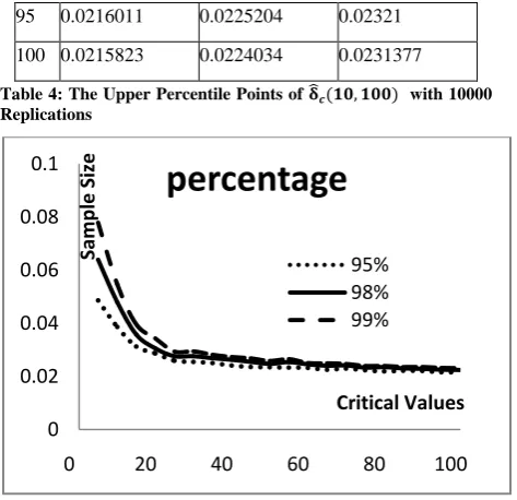
Table 4: The Upper Percentile Points of 𝛅𝒄(𝟏𝟎, 𝟏𝟎𝟎) with 10000
Replications
Fig. 2: The Relation Between Sample Size and Critical Values.
From Table 4 and Fig. 2, the critical values decrease as the sample size increases and they increase as the confidence level increases.
6.
APPLICATIONS
Here, we introduce some of real examples to elucidate the applications of our test in the two cases (censored and non-censored data) of no non-censored data at 95% confidence level.
a-
Case of complete data
In this section, two examples are presented considering s = 0.6, b=0.1.
Example1: Consider the data in Abouammoh et al. (1994) these data represent set of 40 patients suffering from blood cancer (leukemia) from one of ministry of health hospitals in Saudi Arabia and the ordered values in years are:
0.315 0.496 0.616 1.145 1.208 1.263 1.414
2.025 2.036 2.162 2.211 2.370 2.532 2.693
2.805 2.910 2.912 3.192 3.263 3.348 3.348
3.427 3.499 3.534 3.767 3.751 3.858 3.986
4.049 4.244 4.323 4.381 4.392 4.397 4.647
4.753 4.929 4.973 5.074 4.381
It was found that δ𝐿(0.6, 0.1) = 0.31 which is greater than the
critical value of Table 1. Then we conclude that this data set have UBAL property and not exponential.
Example 2: Consider the well-known Darwin data Fisher (1966) that represent the differences in heights between cross and self-fertilized plants of the same pair grown together in one pot:
4.9 −6.7 0.8 1.6 0.6
2.3 2.8 4.1 1.4 2.9
5.6 2.4 7.5 6.0 −4.8
It was found thatδ𝐿(0.6, 0.1) = 0.069 which less than the
critical value of Table 1. Then, we accept the null hypotheses which states that the data set has exponential property.
b-
Case of censored data
In this section, an example is presented considering s = 10, b=100.
Example 3:Consider the data in Mahmoud and Abdul Alim (2008) which represent 51 liver cancers patients taken from Elminia cancer center Ministry of Health { Egypt, which entered in (1999). Of them 39 represent whole life times (non-censored data) and the others represent (non-censored data. The ordered life times (in days) are The ordered non-censored data are
10 14 14 14 14 14 15 17 18
20 20 20 20 20 23 23 24 26
30 30 31 40 49 51 52 60 61
67 71 74 75 87 96 105 107 107
107 116 150
The ordered censored data are:
30 30 30 30 30 60
150 150 150 150 150 185
One can calculate δ𝑐 10, 100 = 0.11 which is greater than the critical value of Table 4. Then we conclude that this data set have UBAL property and not exponential.
7.
ACKNOWLEDGEMENTS
The authors would like to thank the editors and the referees for their valuable comments and suggestions.
8.
REFERENCES
[1] Abouammoh AM., Abdulghani SA., Qamber IS. (1994). On partial orderings and testing of new better than renewal used classes. Reliability Eng. Syst. Safety 43:37– 41.
[2] Abu-Youssef, S. E. and Bakr, M.E. (2014). Some properties of UBACT class of life distribution. J. of Adva. Res. in Appl. Math. 1-9.
[3] Abu-Youssef, S. E. and Bakr, M.E. (2014). A goodness of fit approach to class of life distribution with unknown age. Int. J. of Comp. App., 30-35.
[4] Abu-Youssef, S. E., Mohammed, B. I. and Bakr, M.E. (2014). Nonparametric test for unknown age class of life distributions. Int. J. of Rel. and Appl., 99-110.
[5] Abu-Youssef, S. E., Mohammed, B. I. and Bakr, M.E. (2015). Nonparametric Test for UBACT Class of Life Distribution Based on U-Statistic. J. of adv. of math., 402-411.
[6] Abu-Youssef, S. E. and Bakr, M.E. (2018). Laplace Transform Order for Unknown Age Class of Life Distribution with Some Applications. J. Stat. Appl. Pro. 1-10.
[7] Abu-Youssef, S. E., Nahed, S. A. and Bakr, M.E. (2017). Non Parametric Testing for Unknown age class of life distribution. Submitted.
[8] Abu-Youssef, S. E., Nahed, S. A. and Bakr, M.E. (2017). Used Better than Aged in mgf Ordering Class of Life Distribution with Application of Hypothesis Testing. Submitted.
0
0.02
0.04
0.06
0.08
0.1
0
20
40
60
80
100
Sample
Size
Critical Values
percentage
[image:6.595.61.274.500.593.2]27 [9] Ahmad, I. A. (2004). Some properties of classes of life
distributions with unknown age. J. Statist. Prob., 333-342.
[10] Ahmed H. and Kayid M. (2004). Preservation properties for the Laplace transform ordering of residual lives. Statist. Pap. 583–590.
[11] Alzaid, A. A. (1994). Aging concepts for item of unknown age. Stochastic models, 649-659.
[12] Barlow, R. E. and Proschan, F. (1981). Statistical theory of reliability and life testing: Probability models, To Begin With, Silver Spring, MD.
[13] Bryson, M. C. and Siddiqui, M. M. (1969). Some criteria for aging. J. of Ame. Sta. Ass. 1472-1483.
[14] Denuit M. (2001). Laplace transform ordering of actuarial quantities. Insur Math Econ. 83–102.
[15] Fisher RA. (1966). The design of experiments eight edition. Oliver & Boyd, Edinburgh.
[16] Klefsjo, B. (1983). A useful aging property based on the Laplace transform. J. Appl. Prob. 615–626.
[17] Lee (1990). U-statistics theory and practice. Marcel Dekker, New York.
[18] Mahmoud, M. A. W. and Abdul Alim, A. N. (2008). A Goodness of Fit Approach to for Testing NBUFR (NWUFR) and NBAFR (NWAFR) Properties, Int. J. Reliab. Appl. 125-140.
[19] Mugdadi, A. R. and Ahmad, I. A. (2005). Moment Inequalities Derived from Comparing Life with Its Equlibrium Form. J. Stat. Plann. Inf. 303-317.
[20] Willmot, G.E. and Cai, J. (2000). On classes of lifetime distributions with unknown age. Probab. Eng. Inform. Sci. 473-484