Effectiveness of a Computer Based Syntax Program in Improving the Morphosyntax of Students Who are Deaf/Hard of Hearing

(1)

Georgia State University Georgia State University

ScholarWorks @ Georgia State University

Educational Policy Studies Dissertations Department of Educational Policy Studies

2-12-2010

Power and Bias in Hierarchical Linear Growth Models: More

Measurements for Fewer People

Regine Haardoerfer Georgia State University

Follow this and additional works at: https://scholarworks.gsu.edu/eps_diss

Part of the Education Commons, and the Education Policy Commons

Recommended Citation Recommended Citation

Haardoerfer, Regine, "Power and Bias in Hierarchical Linear Growth Models: More Measurements for Fewer People." Dissertation, Georgia State University, 2010.

https://scholarworks.gsu.edu/eps_diss/57

(2)

This dissertation, POWER AND BIAS IN HIERARCHICAL LINEAR GROWTH MODELS: MORE MEASUREMENTS OF FEWER PEOPLE by REGINE HAARDOERFER, was prepared under the direction of the candidate’s Dissertation Advisory Committee. It is accepted by the committee members in partial fulfillment of the requirements for the degree Doctor of Philosophy in the College of Education, Georgia State University.

The Dissertation Advisory Committee and the student’s Department Chair, as representatives of the faculty, certify that this dissertation has met all standards of excellence and scholarship as determined by the faculty. The Dean of the College of Education concurs.

_________________________ _________________________

Phill Gagné, Ph.D. Paul A. Alberto, Ph.D.

Committee Chair Committee Member

_________________________ _________________________

L. Juane Heflin, Ph.D. Frances A. McCarty, Ph.D.

Committee Member Committee Member

_______________________ Date

_________________________ Sheryl A. Gowen, Ph.D.

Chair, Department of Educational Policy Studies

_________________________ R. W. Kamphaus, Ph.D.

(3)

AUTHOR’S STATEMENT

By presenting this dissertation as a partial fulfillment of the requirements for the

advanced degree from Georgia State University, I agree that the library of Georgia State University shall make it available for inspection and circulation in accordance with its regulations governing materials of this type. I agree that permission to quote, to copy from, or to publish this dissertation may be granted by the professor under whose direction it was written, by the College of Education's director of graduate studies and research, or by me. Such quoting, copying, or publishing must be solely for scholarly purposes and will not involve potential financial gain. It is understood that any copying from or publication of this dissertation which involves potential financial gain will not be allowed without my written permission.

(4)

NOTICE TO BORROWERS

All dissertations deposited in the Georgia State University library must be used in

accordance with the stipulations prescribed by the author in the preceding statement. The author of this dissertation is:

Regine Haardoerfer 705 Vista Leaf Court

Roswell, GA 30075

The director of this dissertation is:

Dr. Phill Gagné

Department of Educational Policy Studies College of Education

(5)

VITA

Regine Haardoerfer

ADDRESS: 705 Vista Leaf Court

Roswell, Georgia 30075

EDUCATION:

Ph.D. 2010 Georgia State University

Educational Policy Studies: Research,

Measurement, Statistics

M.Ed. 2005 Western Governors University

Management and Innovation

2nd State Exam 1999 State of Bavaria

Teaching Secondary Mathematics, Physics, and Computer Science

1st State Exam 1997 University of Erlangen-Nürnberg

Teaching Secondary Mathematics and

Physics

PROFESSIONAL EXPERIENCE:

2006–2010 Graduate Research Assistant

Georgia State University, Atlanta, GA

2003-2005 Private Tutor

2000-2003 IB Teacher, 12th Grade Advisor, and Technology

Coordinator

Atlanta International School

1999-2000 IT Training and Support

Atlanta International School

PROFESSIONAL SOCIETIES AND ORGANIZATIONS:

2006–present American Educational Research Association 2007–present The Association of Teacher Educators 2008-present American Educational Studies Association

PRESENTATIONS AND PUBLICATIONS:

Davis, D. H., Gagné, P., Haardörfer, R., & Waugh, R. E. (2010, May). Examining

reading instruction for students with moderate intellectual disabilities using visual analysis and growth modeling. Paper accepted for presentation at the

annual convention of the Association for Behavioral Analysis International,

(6)

the annual meeting of the American Educational Research Association, Denver, CO.

Haardörfer, R., & Gagné, P. (in press). The use of randomization tests in single-subject

research. Focus on Autism and Other Developmental Disabilities.

Haardörfer, R. (November 2009). International Baccalaureate in a Neoliberal Climate. Paper presented at the Annual Conference for the American Educational Studies Association. Savannah, GA.

Haardörfer, R. (2007). Teacher Autonomy. Paper and Performance presented at the Annual Conference for Curriculum and Pedagogy Group. Austin, TX.

Meyers, B., Swars, S., Schafer, N., Kavanagh, K., Haardörfer, R., Parrish, C., Jacobs, L., Matthews, C., and Taylor, S. (March 2008). Themes and Variations of Critical Friends Groups: A Contextual Look and Virtual Demonstration. Paper presented at the Annual Conference for the American Educational Research. New York, NY.

Meyers, B., Schafer, N., Parrish, C., Taylor, S., Swars, S., Kavanagh, K., Haardoerfer, R., Lick, B., Matthews, S., Jacobs, L. (February 2008). Themes and Variations of Critical Friends Groups: A Contextual Look and a Virtual Demonstration. Paper presented at the Annual Conference for the Association of Teacher Educators, New Orleans, LA.

Schafer, N., Kavanagh, K. Meyers, B., Swars, S., Czaplicki, K., and Haardörfer, R. (April 2009). Virtual Critical Friends Groups: A Vehicle for Professional Development and Supporting Beginning Teachers. Paper presented at the Annual Conference for the American Educational Research. San Diego, CA.

Schafer, N., Meyers, B., Swars, S., Haardörfer, R., Kavanagh, K., and Czaplicki, K. (April 2009). A Comparative Multicase Study Examining the Affordances and Constraints of Critical Friends Groups. Paper presented at the Annual Conference for the American Educational Research. San Diego, CA.

Schafer, N., Meyers, B., Swars, S., Kavanagh, K., Haardoerfer, R., Czaplicki, K.. and Matthews, C. (March 2009). Affordances and Constraints of Critical Friends Groups: Year Two Data of a Longitudinal Comparative Study and Virtual Demonstration. Paper presented at the Annual Conference for the Association of Teacher Educators, Dallas, TX.

(7)

ABSTRACT

POWER AND BIAS IN HIERARCHICAL LINEAR GROWTH MODELS: MORE MEASUREMENTS OF FEWER PEOPLE

by

Regine Haardoerfer

Hierarchical Linear Modeling (HLM) sample size recommendations are mostly made

with traditional group-design research in mind, as HLM as been used almost exclusively

in group-design studies. Single-case research can benefit from utilizing hierarchical linear

growth modeling, but sample size recommendations for growth modeling with HLM are

scarce and generally do not consider the sample size combinations typical in single-case

research. The purpose of this Monte Carlo simulation study was to expand sample size

research in hierarchical linear growth modeling to suit single-case designs by testing

larger level-1 sample sizes (N1), ranging from 10 to 80, and smaller level-2 sample sizes

(N2), from 5 to 35, under the presence of autocorrelation to investigate bias and power.

Estimates for the fixed effects were good for all tested sample-size combinations,

irrespective of the strengths of the predictor-outcome correlations or the level of

autocorrelation. Such low sample sizes, however, especially in the presence of

autocorrelation, produced neither good estimates of the variances nor adequate power

rates. Power rates were at least adequate for conditions in which N2 = 20 and N1 = 80 or

N2 = 25 and N1 = 50 when the squared autocorrelation was .25.Conditions with lower

(8)

(9)

POWER AND BIAS IN HIERARCHICAL LINEAR GROWTH MODELS: MORE MEASUREMENTS OF FEWER PEOPLE

by

Regine Haardoerfer

A Dissertation

Presented in Partial Fulfillment of Requirements of the Degree of

Doctor of Philosophy in

Educational Policy Studies in

the Department of Educational Policy Studies in

the College of Education Georgia State University

(10)

Copyright by Regine Haardoerfer

(11)

ii

TABLE OF CONTENTS

Page

List of Tables ...iii

Chapter 1 INTRODUCTION ...1

2 LITERATURE REVIEW ...6

3 METHOD ...12

4 RESULTS ...15

Conditions With Zero Autocorrelation ...15

Conditions With Nonzero Autocorrelation...38

5 DISCUSSION ...55

Zero Autocorrelation...55

Nonzero Autocorrelation ...57

Recommendations for Single-Case Researchers ...58

Future Research ...59

(12)

iii

1 Biases of Estimating τ00 When N2 = 5 ...16

2 Biases of Estimating τ11 When N2 = 5 ...17

3 Power to Detect β10 When N2 = 5 ...19

5 Power to Detect β10 when N2 = 15 ...20

18 Power to Detect τ00 When ρTimeY = 0.2 and ρXY = 0.2 ...34

(13)

iv

Table Page

22 Biases for τ00 When ρTimeY = .2 and ρXY = .2 and N2 = 5 ...39

29 Biases of 2 e σ When ρTimeY = .2 and ρXY = .2 and N2 = 5...44

32 Biases of 2 auto ρ When ρTimeY = .2 and ρXY = .2 and N2 = 5 ...46

35 Power to Detect τ00 When ρTimeY = .2 and ρXY = .2 and N2 = 15 ...49

38 Power to Detect 2 e σ When ρTimeY = .2 and ρXY = .2 and N1 = 10...51

39 Power to Detect 2 auto ρ When ρTimeY = .2 and ρXY = .2 and N2 = 5 ...52

(14)

1

Single-case research aims to assess the changes in the behavior of participants.

This is accomplished by investigating functional relations between the treatments

(independent variable) and the behaviors (dependent variable). A functional relation is “a

quasi-causative relation between the dependent and independent variables [that] exist[s]

if the dependent variable systematically changes in the desired direction as a result of the

introduction and manipulation of the independent variable” (Alberto & Troutman, 2009,

p. 425). Repeated measures are used to investigate the impact of an intervention or

treatment; that is, study participants are measured frequently on an outcome variable

(behavior) under different conditions.

Single-case research can be categorized as time-series research, which is defined

as

a periodic measurement process on some group or individual and the introduction

of an experimental change into this time series of measurement, the results of

which are indicated by a discontinuity in the measurements recorded in the time

series. (Campbell, Stanley, & Gage, 1966, p. 37)

Primarily, the research participant is compared to her- or himself; comparisons across

individuals are important but generally secondary.

Single-case data sets have specific characteristics. The number of participants is

low; often only a few individuals can be recruited for a study. Furthermore, the number

(15)

2

where two or three waves are most common, but lower than in classical time-series

research, which often produces more than 100 data points.

The traditional approach to analyzing single-case data is visual analysis. The data

are graphed with time on the horizontal axis and the dependent variable on the vertical

axis. Visual analysis investigates the presence and shape of a functional relation between

the treatment and the outcome measure. The focus of the analysis is on the three main

characteristics of single-case data: central location, trend, and variability (Franklin,

Gorman, Beasley, & Allison, 1997). Central location can take on different definitions

such as mean, mode, or median. Trend indicates a systematic, but not necessarily

monotonic, increase or decrease of the outcome over time. Variability assesses the

residuals after central location and trend have been taken into account.

While visual analysis is an established part of single-case data analysis, its critics

debate several issues. Researchers indicate that interrater reliability might be a problem

(Jones, Weinrott, & Vaught, 1978; Matyas & Greenwood, 1990). Furthermore, visual

analysis is successful at keeping Type I errors low, as visual analysts are conservative in

their assessment of a functional relation (Kazdin, 1982). That, however, leads to low

power, especially for small and medium effect sizes.

One proposed approach to remedying these issues is the use of statistical analyses

in addition to visual analysis. Several suggestions have been made over the last few

decades, but more recently, efforts have increased due to changes in federal funding

requirements. Since 2001, the No Child Left Behind (NCLB) Act ("No Child Left Behind

(NCLB) Act of 2001, Pub. L. No. 107-110, § 115, Stat. 1425," 2002) requires studies to

(16)

that involves … objective procedures to obtain reliable and valid knowledge.” ("No Child

Left Behind (NCLB) Act of 2001, Pub. L. No. 107-110, § 115, Stat. 1425," 2002). This

definition excludes studies from receiving federal funding if they rely solely on visual

analysis.

Two schools of thought prevail on the use of statistical analyses for single-case

data. Some researchers advocate non-parametric tests tailored to single-case data. Others

suggest the use of well established group analyses.

Randomization tests are the most popular non-parametric tests that have been

proposed and used in single-case research (Todman & Dugard, 2001). On the surface,

they offer simple methods to determine statistical significance. They are, however,

incompatible with single-case research philosophy and controversial due to

unsubstantiated claims regarding their validity. Their low statistical power only

exacerbates these problems (Haardörfer & Gagné, in press).

Most traditional statistical analyses such as t-tests and ANOVA focus on group

comparisons and condense data into phase averages. The reduction of data into phase

averages results in loss of information regarding individual responses. They are therefore

incongruent with single-case researchers’ interests (Barlow & Hersen, 1984).

Furthermore, such analyses also are based on assumptions that are incongruent with

certain characteristics of single-case data, such as the presence of autocorrelation (also

called serial-dependency), which is a common occurrence when taking many

measurements of the same people in a relatively short amount of time.

Although autocorrelation is an established part of time-series research (Yaffee &

(17)

4

discussions about the presence and impact of autocorrelation. A lengthy discussion

originated in the mid-1980s surrounding the question of whether autocorrelation even

exists in single-case data (Busk & Marascuilo, 1988; Huitema, 1985, 1988; Sharpley &

Alavosius, 1988; Sideridis & Greenwood, 1997; Suen, 1987; Suen & Ary, 1987). This

exchange was started by Huitema’s (1985) claim that autocorrelation is merely a myth.

Several studies investigating the presence of autocorrelation in single-case data ensued,

yielding diverse results. Sideridis and Greenwood (1997) suggest that autocorrelation is

present in only 12% of the baselines of an extensive pool of single-case behavioral

experiments. Bengali and Ottenbacher (1998) encountered autocorrelation more often in

treatment than in baseline phases and with higher values. As time-series methodologists

have pointed out for a long time, in research involving treatment that aims to change

behavior, “serial dependency will coexist” (Sideridis & Greenwood, 1997, p. 290). Thus,

regarding autocorrelation Sideridis and Greenwood appropriately urge researchers that

“whenever statistical analyses are contemplated, its presence should always be

examined” (p. 273).

Some researchers have suggested the use of regression analysis as a way to

analyze single-case data (Allison & Gorman, 1993; Center, Skiba, & Casey, 1985).

Regression analysis does not require as many data points as time-series analysis. One

problem, however, is that regression is inappropriate for nested data. Single-case data are

nested as soon as data are collected from more than one participant; measurements are

nested within people.

Expanding on the idea of regression analysis, methodologists have investigated

(18)

losing the focus on the individual. Several researchers have suggested that hierarchical

linear modeling (HLM) offers a viable option to single-case researchers (Jenson, Clark,

Kircher, & Kristjansson, 2007; Lumpkin, Silverman, Weems, Markham, & Kurtines,

2002; Shadish & Rindskopf, 2007; Van den Noortgate & Onghena, 2003a, 2003b;

Zucker, Schmid, McIntosh, Agostino, Selker, & Lau, 1997). Originally dealing with

cross-sectional nested data (e.g., students in schools), HLM has been expanded to analyze

repeated measures where measurements are nested in individuals. The first level models

the growth of an individual, just as a single-case researcher displays a graph for each

study participant. The second level of the model includes person-level predictors. A third

level can be introduced, if individuals are nested in groups such as classrooms or therapy

groups.

While single-case data fulfill the key requirements to use HLM analyses, the often

small level-2 sample sizes present a challenge. The HLM literature does not offer

recommendations addressing sample sizes in the range of those used by single-case

researchers. While it is widely acknowledged that larger sample sizes on either level yield

better estimates and higher power (Raudenbush & Bryk, 2002; Snijders & Bosker, 1999),

applied researchers have to consider financial and methodological constraints. Thus,

detailed knowledge regarding sufficient sample sizes would be invaluable. The present

study addressed this issue by investigating sample size combinations that are realistic for

single-case research designs featuring many measurements for relatively fewer people

(19)

6

Chapter 2

Literature Review

The majority of HLM power recommendations address cross-sectional studies of

different degrees of model complexity. Recommendations based on analytical approaches

exist for two-level models without level-2 predictors. Raudenbush (1997) provides

formulae to estimate the optimal level-1 (N1) and level-2 (N2) sample size for such

models, including cost factors connected to increasing sample size on either level. A

simulation study by Mok (1995) attempts to address the same questions. Her design

includes a symmetrical use of sample sizes on both levels ranging from 5 to 150,

resulting in total sample sizes ranging from 25 to 22500. Mok’s results indicate that

increasing N2 has a greater positive impact on bias and power than increasing N1. Her

suggestions call for a total sample size of 3500 for an intra-class correlation below .15 to

ensure sufficiently low bias in the estimates. Browne and Draper (2000), however, report

that estimates were close to being unbiased for a total sample size of 216. They

acknowledge that power was not acceptable in this case, but was adequate for a total

sample size of 864. The different results might be attributed to the researchers’ choices in

values for the fixed and random effects.

Beyond the models without level-2 predictors, several authors offer analytical

considerations or formulae for models that include dichotomous predictors at level 2

(O'Connell & McCoach, 2008; Raudenbush, 1997). O’Connell and McCoach offer

recommendations for two- and three-level random-intercept random-slope models.

For these models, the authors provide formulae to estimate sample sizes. They find

(20)

random effects, as does including a cluster-level predictor. For more specific

recommendations, they refer to available power analysis software programs that

require researchers to provide estimates of effect sizes, intra-class correlation, and

proportion of variance explained by the level-2 predictor. Expanding on

Raudenbush’s (1997) earlier work, Raudenbush and Liu (2000) conclude that Mok’s

findings that the number of sites has greater effect than the number of participants per

site also holds true for models with dichotomous predictors at level 2.

Regarding models with one or more non-dichotomous predictors at the second

level, advice on minimum sample sizes is less plentiful. Even established textbook

authors offer little in the way of concrete recommendations. Raudenbush and Bryk

(2002) address the issue of sample size toward the end of the book and only in very

general terms. Kreft and De Leeuw (1998) consider group sizes of 10 to be small and

100 to be large. In addition, they cite three unpublished dissertations that provide

research regarding sample size recommendations. The authors conclude that the total

number of observations is key for level-1 parameter estimates, while the number of

groups has a clear impact on the power of level-2 estimates. They suggest that both

sample sizes should be larger than 30 to detect a cross-level interaction. In addition,

they state that having a larger level-2 sample size has a greater impact on power than

a larger level-1 sample size, holding the total number of measurements constant. In

addition, they contend that a level-2 sample size of 150 leads to a high power (0.90)

for a low level-1 sample size of 5. The authors also mention, however, that a

downward bias in variance estimates is present in level-2 samples of less than 300 for

(21)

intra-8

class correlation play a role in all of these recommendations but do not make mention

of how these factors could or should be taken into account. Snijders and Bosker

(1993) approach the topic analytically and provide the reader with approximation

formulae to estimate optimal sample sizes. Specifically, Snijders and Bosker

recommend N1 to be larger than 10. The researcher, however, needs to provide a lot

of information regarding the data: variance components, means, and covariance

matrices need to be known or estimated to be able to calculate more specific

minimum sample sizes.

Using simulation methods, Maas and Hox (2005) tested scenarios with N2

being 30, 50, or 100, while N1 was 5, 30, or 50. They crossed these possibilities with

three values for intra-class correlations. Their results supported their hypothesis that

any of the given sample size combinations lead to sufficient power. Two more

general Monte Carlo studies regarding cross-sectional HLM have been conducted

recently by Gagné and Estes (2009a, 2009b). In their comprehensive studies, they

tested models with either one predictor at each level or two in one level and one at the

other level. Furthermore, they included a range of predictor-criterion values as well as

presence or absence of cross-level interaction as parameters, thus producing a

controlled correlational structure. Their studies further support the finding that an

increase of sample size at either level increases power but an increase in level-2

sample size has greater impact. Gagné and Estes (2009a) conclude that level-2 sample

sizes smaller than 35 can yield acceptable power with at least 10 measurements per

(22)

The literature regarding minimum sample size recommendation for

hierarchical linear growth models is not plentiful either. The textbook on applied

longitudinal data analysis by Singer and Willet (2003) mentions sample sizes only in

regard to the minimum number of measurements per participant. Two groups of

researchers (Raudenbush & Liu, 2001; Zhang & Wang, 2009) offer advice regarding

sample size recommendations for data with independent error structures. Zhang and

Wang (2009) offer SAS macros to calculate the power given N1, N2, effect size, and

number of participants for linear and quadratic growth models. While the macros can

account for systematic attrition of study participants, they do not include level-2

predictors or non-independent error covariance structures. Sample conditions indicate

that an effect size of 0.2 for the slope might require more than 300 participants when

measured three times and still more than 200 when six measurements are taken per

person. The authors also show power curves dependent on slope effect size which

illustrate that power increases quickly with an increase in effect size.

Raudenbush and Liu (2001) focused on models with a dichotomous level-2

predictor with independent error variance-covariance structures. Like O’Connell and

McCoach (2008), their theoretical work leads them to the general conclusion that an

increase in N1 or N2 increases power. Their recommendations are two-fold:

increasing N1 is best when the degree of the polynomial is high and there is

considerable within-person variance; increasing N2 is best when between-person

heterogeneity is large. Similar to Zhang and Wang (2009), Raudenbush and Liu’s

level-2 sample size recommendations are quite large, ranging from 238 to 800 for an

(23)

10

Hedeker, Gibbons, and Waternaux (1999) also offer analytical solutions for

minimum sample sizes. They focus on non-independent error variance-covariance

structures including compound symmetry, random effect, and autocorrelation. Their

formulae allow the researcher to estimate a minimum level-2 sample size to reach

power of .80 if she knows the level-2 sample size, the effect size, all

predictor-outcome correlations, and the within- and between-group variances. The authors

furthermore offer a table with some pre-calculated minimum sample sizes for level-2

for 4, 6, and 8 measurements, each instance pertaining to a power of .80. The authors

estimate that for 4 waves of data with an autocorrelation of .3, adequate power to

detect a small linear effect necessitates 758 participants. The level-2 sample size

recommendation decreases to 48 with large effect sizes and decreases even further for

larger autocorrelations. Interestingly, in the presence of high autocorrelation, an

increase in level-1 sample size calls for an increase in level-2 sample size to achieve

adequate power.

While the aforementioned researchers focused exclusively on power,

estimation bias is of concern as well. As HLM uses maximum likelihood estimations,

any model misspecification can cause bias in the estimation of fixed and random

effects (White, 1982). Ferron, Daily, and Yi (2002) found that assuming

independence of errors instead of allowing for a nonzero autocorrelation introduces

only a small bias in the estimates of the fixed effects but inflated the error variances

much more. The biases diminish slightly, however, with an increase in level-2 sample

(24)

models than theirs. Kwok, West, and Green (2007) support these findings and add

that the inflation of estimates of the error variances impacts power negatively.

Two recent studies include autocorrelation in their investigation of bias and

power in using HLM for single-case designs (Ferron, Bell, Hess, Rendina-Gobioff, &

Hibbard, 2009; Jenson et al., 2007). Both focus on the most basic building block of

single subject design (Alberto & Troutman, 2009), the AB design. The model

includes one level-1 predictor, a dummy variable, to indicate the beginning of the

treatment phase. No level-2 predictors were considered. Ferron et al. (2009) indicate

that power was high for very small sample sizes of 4 measurements and 10

participants, though lower in the presence of autocorrelation. Jenson, Clark, Kircher,

and Kristjansson (2007), however, report that power was not sufficient for 15

participants, with 5 baseline and 10 treatment measurements, with or without

autocorrelation. Their simulations suggest that even having 10 baseline and 20

treatment measures for 15 people does not yield adequate power for autocorrelations

of .40 and .80. The discrepancies are likely due to the researchers’ different choices

for the value of the fixed and random effects.

In conclusion, sample size recommendations are fairly common for

cross-sectional HLM, scarce for growth modeling including complex models, and emerging

for single-case models. The purpose of the present study was to expand sample size

recommendations in hierarchical growth modeling to larger numbers of

measurements and smaller numbers of participants. It focused on a two-level model

with one continuous level-1 predictor and one continuous level-2 predictor. The

(25)

12

Chapter 3

Method

This is a Monte Carlo simulation with five independent variables: the level-1

sample size (i.e., number of measurements per participant), the level-2 sample size (i.e.,

the number of participants), the magnitude of the autocorrelation factor of the level-1

error with lag 1, the magnitude of the interpredictor correlation, and the magnitude of the

correlation between Time and the outcome variable Y. Data were simulated for a

hierarchical model reflecting linear growth with one level-2 predictor for the intercept

and the same level-2 predictor for the level-1 slope, as illustrated in the following

equations for the level-1, level-2, and combined models

ti 0i 1ij ti ti

Y =π +π (TIME )+e

0i 00 01 i 0i

1i 10 11 i 1i π β +β X +r

π β +β X +r

= =

or

ti 00 01 i 10 ti 11 i ti 0i 1i ti ti

Y =β +β (X )+β (TIME )+β (X )(TIME )+r +r (TIME )+e .

Single-case data do not meet the assumption that eti is normally distributed with a

mean of 0 and a variance of σe2. Instead, single-case researchers have to assume that the

level-1 errors are autocorrelated. Most common is a lag of one, meaning that any

consecutive error is autocorrelated with the error of the previous measurement,

t 1)i (t ti ρe ν

e = ₋ + .

In this formula, ρ represents the constant autocorrelation factor with an absolute value

(26)

2 2 ν 2 e ρ 1 σ σ − = ,

where σe2 denotes the apparent, and inflated, error variance as it would be detected if

the analysis were not to look for the possibility of autocorrelation of the level-1

errors; σν2 is the actual level-1 error variance in the data.

SAS 9.1 (SAS Institute, 2004) was used to generate the data and to conduct all

calculations and analyses. For each combination of parameters, 1,000 replications

were conducted, with the data being simulated in IML and then analyzed using the

following PROC MIXED routine (Littell, Milliken, Stroup, Wolfinger, &

Schabenberger, 2006; Singer, 1998):

PROC MIXED DATA=CompleteDataSet COVTEST NOCLPRINT NOITPRINT NOINFO IC;

CLASS ID Wave;

MODEL Y = Time X TimeX /DDFM=BW CL NOTEST; RANDOM Intercept Time /SUB=ID TYPE=UN;

REPEATED Wave /SUB=ID TYPE=AR(1); RUN;

To simplify the situation, time points were spaced equally. Thus, the level-1

sample size was directly proportional to the duration of the “study.” For ease of

interpretation, the spacing was 1. In addition, the level-2 predictor was grand-mean

centered, and Time was simulated such that Time = 0 at the midpoint of the

measurement occasions.

A broad range of sample sizes pertinent to single-case research was

investigated. The level-1 sample size took on seven different values: 10, 15, 20, 30,

40, 50 and 80. The level-2 sample sizes, reflecting the number of participants, were 5,

(27)

14

autocorrelation factors were chosen so that their squares were .05, .10, .15, .20, and

.25. Time and the outcome variable were correlated at .2, .3, .4, and .6. The

correlation between the level-2 predictor and the outcome variable was set to .2 and

.3. The correlation between the cross-level interaction and the outcome variable was

fixed at .3, and the correlation between Time and the level-2 predictor was fixed at 0.

These parameters lead to 36 x 6 x 4 x 2 conditions and thus to 1728 cells.

Power for each set of parameters was calculated as the percentage of betas

that are identified as statistically significant. Power results ranging from 0.80 to 0.90

were considered acceptable, while power greater than 0.90 was considered high.

Relative bias in parameter estimates was considered low if it is below 5%, and

relative bias less than 10% in the standard errors was considered low (Hoogland &

Boomsma, 1998), and it was calculated as

. 100 * parameter

parameter

-estimate parameter

(28)

15

The results regarding the biases of the estimates are presented in color-coded

tables. The color green is used for magnitudes below 5%. Yellow illustrates biases with

magnitudes between 5% and 10%. Orange signifies conditions in which the magnitudes

of the biases exceeded 10%.

For all power tables, the cells shaded in green indicate high power that is power of

at least .90 but less than 1. Perfect power, a power of 1, is marked dark green. Yellow

signifies conditions in which power was adequate, defined as at least .80 and below .90.

Any cells marked indicate inadequate power, or values below .80.

Conditions With Zero Autocorrelation

Biases. In general, the estimates of the fixed and random values were neither

dependent upon the strength of the correlation between Time and the outcome variable

nor between X and Y for any of the conditions tested. The variations in biases of the

estimates when autocorrelation had been set to 0 only varied due to differences in sample

size combinations. As expected, an increase in either level-1 or level-2 sample size

improved the accuracy of the estimates of the fixedand the random effects.

For the conditions tested with autocorrelation of errors set at 0, the fixed effects

(β00,β01,β10, andβ11) were all estimated with the absolute values of the biases below 5%

when N2 was at least 10, independent of the strength of the correlation between the

predictors. The magnitudes of 9 of the 192 biases were slightly above 5% when N2 = 5

(29)

16

For the conditions examined, the biases for the level-2 error variances (τ00 and τ11)

were below 5% for sample size combinations with a total sample size GrandN (N1xN2)

larger than 150. The biases were especially large for conditions with a level-2 sample size

of 5 (Tables 1 and 2). As level-1 sample sizes increased, however, the biases decreased

quickly for both level-2 variances. With N2 = 5 and N1 = 50, biases were below or

around 5%. At a level-1 sample size of 80, the magnitudes of the bias were all below 5%.

Table 1

Biases of Estimating τ00 When N2 = 5

Level-1 Sample Size

ρXY ρTimeY 10 15 20 30 50 80

.2 25.8439 15.3692 9.3136 8.6327 5.1587 3.6403

.3 28.6305 16.4368 13.3016 6.3959 4.9817 2.1879

.4 26.9261 15.7487 13.7419 7.7229 3.1964 1.4446

.2

.6 32.3837 12.9452 12.303 9.3636 2.7376 -0.7201

.2 30.5126 17.8394 14.4369 5.6151 1.312 4.0045

.3 28.0941 12.9102 10.9528 6.0016 7.732 2.777

.4 26.9775 18.3079 7.1991 4.482 1.3091 0.1018

.3

(30)

Table 2

Biases of Estimating τ11 When N2 = 5

Level-1 Sample Size

ρXY ρTimeY 10 15 20 30 50 80

.2 32.8617 18.8305 12.5967 7.6518 4.8994 2.919

.3 29.86 14.6556 13.929 9.8568 4.0105 0.3235

.4 30.0971 13.758 13.0104 4.916 0.7321 2.9474

.2

.6 37.9955 17.9014 13.193 3.2803 3.5469 0.9802

.2 36.0297 18.146 10.1988 5.9091 3.0259 1.8507

.3 34.8824 13.5734 10.1184 6.7328 5.0199 3.2689

.4 33.8035 18.8711 11.3961 5.3816 -0.3078 3.98

.3

.6 29.8537 21.3782 15.0326 10.9989 2.0832 2.9362

With N1 = 10 and N2 = 10, about half of the bias values were above 5%. In

addition, many biases for (10, 15)1 or (15, 10) as a sample size combination were

between 5% and 10%. Furthermore, neither an increase in the correlation between Time

and the outcome variable nor an increase in the correlation between X and the outcome

variable seemed to impact the variance estimation of the level-2 variances.

The level-1 error variances were all estimated with biases below 5% for all

conditions tested for which the autocorrelation was 0. The strength of the

predictor-outcome variables had no influence on the estimates. The sample sizes tested were all

sufficiently large to produce good estimates of the level-1 variance.

(31)

18

Power. In all but two of the tested conditions with zero autocorrelation, the power

to detect β00 was perfect, that is 100%. When N2 was 5 and N1 was 30, power decreased

to 99.9% under the lowest correlation condition. The same result applied to the

conditions in which both predictor-outcome correlations were set at .3 and the sample

size combination was (5, 30). Power of the other fixed effects varied depending on the

sample size combinations as well as the predictor-outcome correlations. Thus, they will

be discussed separately in more detail.

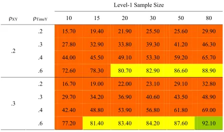
Power to detect β10. In general, power to detect β10 was similar for the two tested

correlations between X and Y, with power values being slightly larger for the larger X-Y

correlation. As expected, the value of the correlation between Time and Y had greater

influence on the power to detect β10. For the lowest level-2 sample size of 5, power was

only adequate for the highest correlation between Time and the outcome variable (Table

3). When ρTimeY was set to .6, however, sample sizes of 15 and above yielded power

greater than .8. Notably, when N2 was only 5 and the highest correlation combination

(32)

[image:32.612.101.548.131.395.2]

Table 3

Power to Detect β10 When N2 = 5

Level-1 Sample Size

ρXY ρTimeY 10 15 20 30 50 80

.2 15.70 19.40 21.90 25.50 25.60 29.90

.3 27.80 32.90 33.80 39.30 41.20 46.30

.4 44.00 45.50 49.10 53.30 59.20 65.70

.2

.6 72.60 78.30 80.70 82.90 86.60 88.90

.2 16.70 19.00 22.00 23.10 29.10 32.80

.3 29.70 34.20 36.90 40.60 43.50 48.90

.4 42.40 48.80 53.90 56.80 61.80 69.00

.3

.6 77.20 81.40 83.40 84.20 87.60 92.10

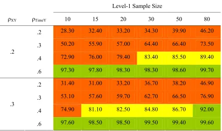
Level-2 sample sizes of 10 and 15 produced high power rates when the

correlation between Time and the outcome variable was large. Specifically, with N2 = 10

and ρTimeY = .6, power was above 90% for all tested level-1 sample sizes and X-Y

correlations (Table 4). Independent of ρXY, when ρTimeY was .4, most conditions showed

adequate or high power; when ρTimeY was .2 or .3, no conditions produced adequate power

to detect β10. Power rates increased when N2 was 15. Almost all conditions with ρTimeY of

(33)

[image:33.612.100.550.114.703.2]

20

Table 4

Level-1 Sample Size

ρXY ρTimeY 10 15 20 30 50 80

.2 28.30 32.40 33.20 34.30 39.90 46.20

.3 50.20 55.90 57.00 64.40 66.40 73.50

.4 72.90 76.00 79.40 83.40 85.50 89.40

.2

.6 97.30 97.80 98.30 98.30 98.60 99.70

.2 31.40 31.00 33.20 36.70 38.20 46.90

.3 53.10 57.60 59.70 62.70 66.50 76.90

.4 74.90 81.10 82.50 84.80 86.70 92.00

.3

.6 97.60 98.50 98.50 99.50 99.40 99.60

Table 5

Power to Detect β10 when N2 = 15

Level-1 Sample Size

ρXY ρTimeY 10 15 20 30 50 80

.2 37.90 42.60 44.80 45.80 53.10 61.40

.3 67.80 72.30 75.40 77.70 82.10 87.10

.4 89.00 91.10 92.30 94.90 94.70 98.30

.2

.6 99.50 99.80 99.80 100.00 100.00 100.00

.2 39.80 43.30 44.20 47.80 54.10 62.40

.3 70.50 75.10 77.40 80.50 83.70 89.00

.4 90.80 92.20 93.60 96.10 96.10 98.10

.3

[image:33.612.103.548.115.378.2]

(34)

With N2 = 20 and ρTimeY = .6, almost all tested level-1 sample sizes yielded

perfect power. Furthermore, when ρTimeY was .4, power was always above 90%. Even for

ρTimeY = .3, all but the condition with the lowest values for N1 and ρXY had adequate or

high power. None of the conditions with ρTimeY = .2 had adequate power with 20

participants.

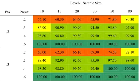
Within a set of predictor-outcome correlations, power increased slowly with an

increase in N2 (Table 6). This was especially pronounced for ρTimeY = .2. For conditions

in which N2 ≥ 25, N1 ≥ 15, and ρTimeY≥ .3 power was high. When only 10 measurements

(35)

[image:35.612.102.550.131.391.2]

22

Table 6

Level-1 Sample Size

ρXY ρTimeY 10 15 20 30 50 80

.2 55.10 60.30 64.60 65.90 71.80 80.30

.3 86.90 90.90 90.90 94.50 95.80 97.90

.4 98.80 98.80 99.30 99.50 99.60 99.90

.2

.6 100.00 100.00 100.00 100.00 100.00 100.00

.2 60.00 62.30 66.10 69.30 74.50 82.10

.3 88.40 92.90 92.60 95.50 97.70 98.60

.4 98.30 98.80 99.70 99.40 100.00 100.00

.3

.6 100.00 100.00 100.00 100.00 100.00 100.00

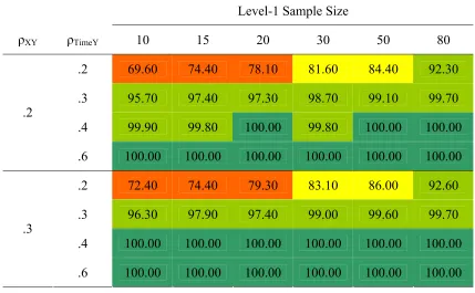
Even for the highest tested level-2 sample size of 35 (Table 7), power was not

adequate for conditions where ρTimeY was .2 and N1 was less than 30. It was, however

(36)

[image:36.612.100.529.131.396.2]

Table 7

Level-1 Sample Size

ρXY ρTimeY 10 15 20 30 50 80

.2 69.60 74.40 78.10 81.60 84.40 92.30

.3 95.70 97.40 97.30 98.70 99.10 99.70

.4 99.90 99.80 100.00 99.80 100.00 100.00

.2

.6 100.00 100.00 100.00 100.00 100.00 100.00

.2 72.40 74.40 79.30 83.10 86.00 92.60

.3 96.30 97.90 97.40 99.00 99.60 99.70

.4 100.00 100.00 100.00 100.00 100.00 100.00

.3

.6 100.00 100.00 100.00 100.00 100.00 100.00

Overall, the correlation between Time and the outcome variable had great

influence on power to detect β10. This was expected as β10 is the fixed effect that models

the level-1 predictor’s direct influence on the outcome variable. The magnitude of ρXY

(37)

24

Power to detect β01. Within any correlation combination, the power to detect β01

increased with an increase in either level-1 or level-2 sample size. It also increased with

an increase in the correlation between the level-2 predictor X and the outcome variable

Y, that is, the correlation associated with β01. Furthermore, an increase in the correlation

between the Time and the outcome variable increased the power of β01 as well. This

increase, however, was not as strong as the one related to the increase in ρXY.

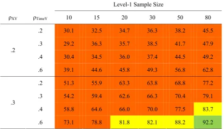
Power to detect β01 under conditions in which N2 = 5 was extremely low, ranging

from 17.7% for the lowest level-1 sample size and lowest correlation combination to a

still low 65.1% for the highest level-1 sample size and highest correlation combination.

Additionally, when the correlation between the level-2 predictor and the outcome

variable was set to .2, power was inadequate for all conditions with a level-2 sample size

of either 10 or 15. For a correlation between X and Y of .3, power was at least adequate

for more than half of the tested conditions, with values increasing with an increase in

level-1 sample size or an increase in the correlation between Time and the outcome

variable. In conditions when 80 measurements were simulated for 15 participants, power

was high at all values tested of the correlation between Time and Y. Also, when the

Time-Y correlation was set to .6, taking at least 15 measurements produced high power.

The specific power results for N1 of 10 and 15 are presented in Table 8 and Table 9,

(38)

[image:38.612.102.550.132.391.2]

Table 8

Level-1 Sample Size

ρXY ρTimeY 10 15 20 30 50 80

.2 30.1 32.5 34.7 36.3 38.2 45.5

.3 29.2 36.3 35.7 38.5 41.7 47.9

.4 30.4 34.5 36.0 37.4 44.5 49.2

.2

.6 39.1 44.6 45.8 49.3 56.8 62.8

.2 51.3 55.9 63.3 63.8 68.8 77.2

.3 54.2 59.4 62.6 66.3 70.4 79.1

.4 58.8 64.6 66.0 70.0 77.5 83.7

.3

(39)

26

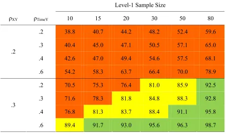
[image:39.612.102.548.131.395.2]

Table 9

Level-1 Sample Size

ρXY ρTimeY 10 15 20 30 50 80

.2 38.8 40.7 44.2 48.2 52.4 59.6

.3 40.4 45.0 47.1 50.5 57.1 65.0

.4 42.6 47.0 49.4 54.6 57.5 68.1

.2

.6 54.2 58.3 63.7 66.4 70.0 78.9

.2 70.5 75.3 76.4 81.0 85.9 92.5

.3 71.6 78.3 81.8 84.8 88.3 92.8

.4 76.8 81.3 83.7 88.4 91.1 95.8

.3

.6 89.4 91.7 93.0 95.6 96.3 98.7

For a level-2 sample size of 20 (Table 10), power was never high when ρXY was

.2 and ρTimeY was .6. It reached adequate values for level-1 sample sizes of 50 and 80.

Power increased substantially when ρXY was increased to .3. All conditions in which ρXY

(40)

[image:40.612.102.548.131.396.2]

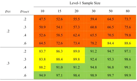
Table 10

Level-1 Sample Size

ρXY ρTimeY 10 15 20 30 50 80

.2 47.5 52.6 55.5 59.4 64.5 73.7

.3 50.9 54.1 57.3 60.8 66.5 75.6

.4 52.6 58.5 62.4 65.5 70.5 79.8

.2

.6 64.5 72.6 73.4 78.2 84.4 88.6

.2 83.7 86.3 89.0 91.2 94.7 97.1

.3 83.8 88.4 89.8 92.4 95.3 98.6

.4 88.2 91.0 91.2 94.8 96.8 99.1

.3

.6 94.9 97.1 98.4 98.9 99.7 99.9

When N2 was 25, power increased such that it was at least adequate for N1 = 80

and ρXY = .2 for all tested Time-outcome correlations. In the case of a high correlation of

.6 between Time and Y and the low correlation of .2 between X and Y, power was

adequate starting at a level-1 sample size of 15 and high when N1 was at least 50. When

ρXY was increased to .3, all but the lowest sample size combination had high power. For

N1 of either 50 or 80 and the correlation between Time and Y being at least .4, power

(41)

[image:41.612.101.548.138.375.2]

28

Table 11

Level-1 Sample Size

ρXY ρTimeY 10 15 20 30 50 80

.2 53.7 61.8 61.8 69.8 71.8 82.1

.3 60.7 64.9 68 73.3 76.7 84.0

.4 63.0 67.7 70.8 74.0 80.1 87.0

.2

.6 76.7 80.9 83.2 87.6 91.7 95.1

.2 89.0 92.1 94.9 96.6 98.2 99.0

.3 90.9 94.4 95.1 97.7 97.2 99.8

.4 94.3 95.9 96.4 98.5 99.4 99.6

.3

.6 99.2 99.4 99.5 99.8 100 100

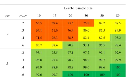
Table 12

Level-1 Sample Size

ρXY ρTimeY 10 15 20 30 50 80

.2 65.5 69.4 73.5 75.8 82.2 87.5

.3 64.1 71.0 76.4 80.0 86.5 89.9

.4 71.5 76.3 78.5 82.4 87.5 93.2

.2

.6 83.7 88.4 90.7 93.1 95.5 98.4

.2 95.1 95.5 97.1 97.2 99.1 99.9

.3 95.8 97.4 98.7 98.2 99.7 99.9

.4 97.9 98.9 98.8 99.6 99.6 100

.3

[image:41.612.103.550.442.712.2]

(42)

For a level-2 sample size of 30 or 35, all Time-Y correlations produced high or

perfect power when ρXY = .3. For the conditions when ρXY was .2, power increased

further with increasing level-1 sample size and ρTimeY. When N2 was 35, all conditions

with N1 being at least 20 produced adequate or high power. For a Time-outcome

correlation of .6, all tested values of N1 produced adequate or high power (Table 13).

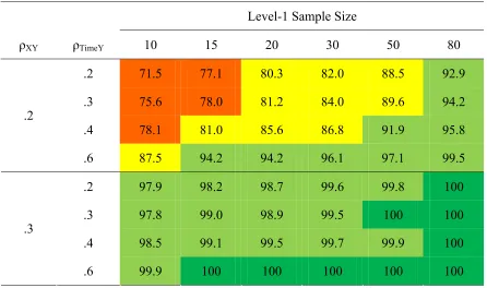
[image:42.612.102.548.264.528.2]

Table 13

Level-1 Sample Size

ρXY ρTimeY 10 15 20 30 50 80

.2 71.5 77.1 80.3 82.0 88.5 92.9

.3 75.6 78.0 81.2 84.0 89.6 94.2

.4 78.1 81.0 85.6 86.8 91.9 95.8

.2

.6 87.5 94.2 94.2 96.1 97.1 99.5

.2 97.9 98.2 98.7 99.6 99.8 100

.3 97.8 99.0 98.9 99.5 100 100

.4 98.5 99.1 99.5 99.7 99.9 100

.3

.6 99.9 100 100 100 100 100

Overall, the correlation between X and the outcome variable had great influence

on power to detect β01. This was expected as β01 is the fixed effect that models the level-2

predictor’s direct influence on the outcome variable. When ρXY was .3, all conditions with

a level-2 sample size of 20 or higher produced adequate or high power. In conditions with

the lower correlation between the level-2 predictor and Y, only larger values of N1 and

(43)

30

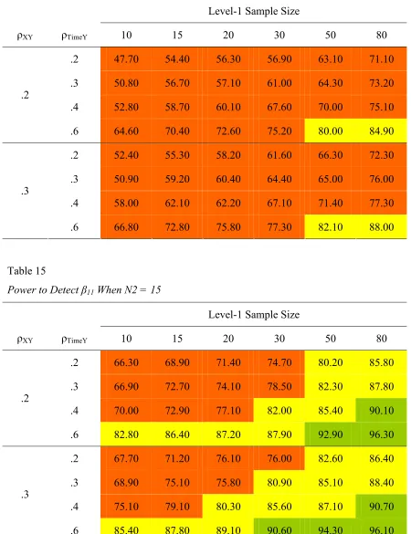
Power to detect β11. In general, the correlation between Time and the outcome

variable (ρTimeY) had more impact on the power to detect β11 than the correlation between

X and Y. Specifically, power was inadequate for all conditions tested where N2 was 5.

Even for the highest correlation combination (ρTimeY = .6 and ρXY = .3), power to detect

β11 was only 62%. When N2 was doubled to 10 (Table 14), only two conditions produced

adequate power (ρTimeY = .6 and N1 > 50). When the level-2 sample size was increased to

15, power increased appreciably (Table 15). All conditions with a Time-Y correlation of

at least .6 or at least 50 measurement occasions produced power rates above 80%.

This trend of increasing power continued with the increase of the level-2 sample

size. For those conditions where N2 was 20, all but two conditions produced at least

adequate power; for half of them, power was high. Furthermore, 42 conditions with N2 =

25 produced high power; the other 6 conditions produced adequate power (Table 16).

When N2 ≥ 30 power rates to detect the interaction effect were all high; more

specifically, all power rates were above 94.9 %. Seven of the conditions with the highest

number of measurements per person and higher predictor-outcome correlations reached

(44)

[image:44.612.100.550.115.700.2]

Table 14

Level-1 Sample Size

ρXY ρTimeY 10 15 20 30 50 80

.2 47.70 54.40 56.30 56.90 63.10 71.10

.3 50.80 56.70 57.10 61.00 64.30 73.20

.4 52.80 58.70 60.10 67.60 70.00 75.10

.2

.6 64.60 70.40 72.60 75.20 80.00 84.90

.2 52.40 55.30 58.20 61.60 66.30 72.30

.3 50.90 59.20 60.40 64.40 65.00 76.00

.4 58.00 62.10 62.20 67.10 71.40 77.30

.3

.6 66.80 72.80 75.80 77.30 82.10 88.00

Table 15

Level-1 Sample Size

ρXY ρTimeY 10 15 20 30 50 80

.2 66.30 68.90 71.40 74.70 80.20 85.80

.3 66.90 72.70 74.10 78.50 82.30 87.80

.4 70.00 72.90 77.10 82.00 85.40 90.10

.2

.6 82.80 86.40 87.20 87.90 92.90 96.30

.2 67.70 71.20 76.10 76.00 82.60 86.40

.3 68.90 75.10 75.80 80.90 85.10 88.40

.4 75.10 79.10 80.30 85.60 87.10 90.70

.3

[image:44.612.104.548.116.378.2]

(45)

32

Table 16

Level-1 Sample Size

ρXY ρTimeY 10 15 20 30 50 80

.2 86.30 87.90 91.30 92.80 95.40 97.70

.3 87.90 89.50 92.00 92.60 95.80 97.90

.4 90.00 93.30 93.40 95.10 97.00 99.10

.2

.6 95.10 97.30 97.80 98.70 98.80 99.60

.2 85.40 91.00 91.90 94.40 96.60 97.90

.3 88.90 92.30 93.20 94.60 96.50 98.20

.4 90.50 91.70 95.50 96.70 98.10 98.70

.3

.6 97.10 98.90 98.70 99.30 98.70 99.70

Table 17

Level-1 Sample Size

ρXY ρTimeY 10 15 20 30 50 80

.2 94.90 96.30 97.20 97.90 98.70 100.00

.3 95.80 97.00 98.50 99.00 99.20 99.80

.4 97.10 97.00 98.10 99.20 99.50 99.90

.2

.6 98.60 99.30 99.80 99.80 100.00 100.00

.2 95.00 98.50 97.70 98.00 99.30 99.80

.3 95.80 98.30 99.20 99.50 99.40 99.90

.4 96.50 98.70 99.00 99.70 99.50 100.00

.3

(46)

Overall, both predictor-outcome correlations had great impact on the power to

detect β11. This was expected as β11 is the fixed effect that models the influence of the

cross-level interaction on the outcome variable. All conditions with N2 ≥ 25 produced at

least adequate power to detect β11.

Power to detect the level-2 variances. Changing the correlations between the

outcome variable and either predictor had no discernable effect on the power of detecting

τ00 or τ11. To illustrate this, the results for the combination of the lowest and highest

correlations are presented. Tables 18 and 19 show the pattern of the power to detect τ00

for the lowest and highest predictor-outcome correlation combinations tested. Tables 20

and 21 illustrate the pattern for τ11.

For the conditions tested, the power to detect τ00 depended upon the level-1 and

level-2 sample size. Power was 0 for all conditions where N2 was 5. Doubling N2 to 10

did not improve the situation; power was still less than 1% even for large level-1 sample

sizes. Increasing N2 beyond 10 produced rapid increases in power, with the majority of

conditions reaching adequate, high, or perfect power. Increasing the level-1 sample size

to at least 30 did allow for adequate or high power for N2 = 15. When N2 = 25, 15

measurements were sufficient for high power. For the lowest level-1 sample size of 10,

adequate power was reached for the two highest level-2 sample sizes tested. In addition,

no conditions tested in which N1 = 10 reached power rates above 90%. Overall, high

power was achieved in more than 25% of the conditions; perfect power was reached for

about a quarter of the tested conditions. In general, power increased faster with an

(47)

34

Table 18

Power to Detect τ00 When ρTimeY = 0.2 and ρXY = 0.2

N1

N2 10 15 20 30 50 80

5 0.00 0.00 0.00 0.00 0.00 0.00

10 0.00 0.00 0.00 0.00 0.10 0.50

15 18.90 40.50 61.40 85.40 96.90 99.70

20 48.00 79.10 92.80 99.00 99.90 100.00

25 70.70 91.40 98.10 99.80 100.00 100.00

30 82.90 97.20 99.50 100.00 100.00 100.00

[image:47.612.105.440.119.393.2]

35 88.40 99.60 100.00 100.00 100.00 100.00

Table 19

N1

N2 10 15 20 30 50 80

5 0.00 0.00 0.00 0.00 0.00 0.00

10 0.00 0.00 0.00 0.00 0.10 0.40

15 19.90 41.40 61.80 86.00 97.00 99.80

20 49.90 79.10 91.20 99.20 100.00 100.00

25 69.20 93.20 98.00 100.00 100.00 100.00

30 80.20 96.40 99.50 100.00 100.00 100.00

(48)

Power to detect τ11 was very similar to detecting power for τ00. The only condition

which produced adequate power for τ11 but not τ00 was the sample size combination of

(15, 20). Also, perfect power for τ11 was reached for fewer conditions with a level-1

sample size of 30.

Table 20

N1

N2 10 15 20 30 50 80

5 0.00 0.00 0.00 0.00 0.00 0.00

10 0.00 0.00 0.00 0.00 0.00 0.30

15 19.40 42.10 60.90 86.90 97.70 99.50

20 49.60 80.40 91.80 99.10 100.00 100.00

25 71.90 93.90 98.10 99.80 100.00 100.00

30 82.80 97.80 99.30 99.90 100.00 100.00

(49)

[image:49.612.104.422.127.362.2]

36

Table 21

N1

N2 10 15 20 30 50 80

5 0.00 0.00 0.00 0.00 0.00 0.00

10 0.00 0.00 0.00 0.00 0.00 0.60

15 18.90 43.00 64.80 85.50 97.80 99.00

20 50.40 81.00 91.20 98.20 100.00 100.00

25 70.00 93.20 98.20 99.80 100.00 100.00

30 83.40 97.90 99.70 100.00 100.00 100.00

(50)

Power to detect the level-1 variance. Under all conditions tested with N2 ≥ 10,

power to detect the level-1 variance was perfect, independent of the predictor-outcome

correlations and sample sizes. When the level-2 sample size was set to 5, some of the

conditions produced power slightly less than perfect. This occurred when the level-1

sample size was either 10 or 15. Under these conditions, power rates were above 99%.

Type I Error Rates. For τ01, all Type I error rates were below 5%, irrespective of

correlations and sample sizes. Increasing the level-1 sample size had no discernable

effect on the Type I error rates for τ01. For all conditions with N2 being 10, the Type I

error rate was 0.10% or 0%. The error rates increased steadily with the increase of N2 for

all tested conditions. The pattern does not indicate whether increasing N2 beyond the

chosen maximum could produce undesirably high Type I error rates for τ01.

The Type I error rate of the autocorrelation factor was around the expected 5% (M

= 5.08, SD = 0.706), but slightly inflated. It was not influenced by any of the variables

that were varied in this study. This means that neither the sample size combination nor

the strengths of the predictor-outcome correlations had any impact on the Type I error

(51)

38

Conditions With Nonzero Autocorrelation

Biases. For the conditions tested where N2 was greater than 5, the biases of the

fixed effects were all below 5% regardless of the magnitude of the autocorrelation factor.

For those conditions where N2 was 5, most biases were below 5%. Some values

exceeded 5% but all were below 10%. No discernable pattern that could explain the

marginally inflated biases was present.

Conditions tested with nonzero autocorrelation showed inflated estimates for the

level-2 error variances τ00 and τ11 when the total sample size was small (Table 15). The

inflation of the biases increased further for conditions with non-zero autocorrelation.

Furthermore, the higher the autocorrelation, the higher was the inflation of the estimates

of the level-2 variances. Therefore, more conditions produced biases of τ00 and τ11 beyond

5% and 10%. Under the highest tested autocorrelation, all biases of τ00 were greater than

10% for a level-1 sample size of 10. The average inflation of the intercept variance τ00 for

the lowest sample size combination and the highest autocorrelation factor tested was

above 75%.

For all conditions tested in which N2 = 5, the biases were inflated. Only large

level-1 sample sizes produced biases in the estimates of τ00 that were around or below

5%. Biases were below 5% in less than 7% of the conditions. This was not achieved for

the conditions with 2

auto

(52)

[image:52.612.105.526.113.340.2]

Table 22

Biases for τ00 When ρTimeY = .2 and ρXY = .2 and N2 = 5

N1

2

auto

ρ 10 15 20 30 50 80

0 25.844 15.370 9.314 8.633 5.159 3.640

.05 47.755 32.310 21.220 13.293 6.617 5.247

.10 66.169 43.448 30.904 11.870 7.859 5.336

.15 76.404 50.191 35.433 27.589 12.462 4.036

.20 99.842 60.467 54.616 30.933 19.731 8.956

.25 114.653 80.138 57.789 39.523 17.803 12.000

Increasing the level-2 sample size to 10 produced more than 63% of the tested

conditions with desirable levels of biases. The conditions with the highest 2

auto

ρ needed 50

or 80 measurements per person to decrease the biases below 5%. No conditions with (10,

(53)

40

[image:53.612.101.524.137.341.2]

Table 23

N1

2

auto

ρ 10 15 20 30 50 80

0 8.4221 1.651 1.097 1.167 0.959 -0.808

.05 20.441 4.384 0.835 1.153 0.440 1.053

.10 24.220 13.115 2.336 1.900 -0.161 7.197

.15 38.101 13.791 8.534 6.077 1.184 -2.390

.20 52.315 22.454 12.528 2.828 4.783 -0.970

.25 75.270 29.266 17.738 10.608 0.431 2.968

For even higher level-2 sample sizes, the impact of the autocorrelation factor on

the intercept variance estimates lessened (Table 24). The effect decreased further for N2

= 25 to the point where only conditions with high levels of autocorrelation and a level-1

(54)

Table 24

N1

2

auto

ρ 10 15 20 30 50 80

0 0.405 -0.713 -2.884 -0.164 -0.954 0.134

.05 7.913 1.777 1.388 0.731 -0.005 -0.502

.10 13.699 4.604 2.604 2.210 -1.070 -0.158

.15 17.727 9.525 -0.113 0.996 0.336 -0.318

.20 28.868 12.998 3.179 1.157 -0.359 0.198

[image:54.612.99.523.427.639.2]

.25 42.742 15.116 6.565 4.346 1.477 -1.020

Table 25

N1

2

auto

ρ 10 15 20 30 50 80

0 0.820 0.001 -0.975 -0.362 -1.534 -0.281

.05 4.930 -0.570 -1.382 1.285 0.663 0.081

.10 4.188 0.597 -2.657 -0.354 0.017 0.365

.15 7.937 -0.462 -2.346 -0.789 -0.870 -1.618

.20 13.691 2.467 -2.126 -0.299 -0.865 -0.377

.25 21.828 1.495 -0.594 -0.299 -0.878 1.3044

For larger level-2 sample sizes, the pattern continued. When N2 = 30, two values

(55)

42

the lowest level-1 sample size produced an undesirably large bias in the intercept

variance.

The biases for the slope variance τ11 behaved similarly to those of the intercept

variance. The higher the autocorrelation was, the greater was the inflation of the

estimates. Increasing the level-2 sample size produced more conditions with desirable

biases below 5%. For identical conditions the biases for τ11 were lower than those for τ00

(Tables 26 – 28). For all conditions in which the level-2 sample size was 25 or larger, all

biases for the intercept variance were below 5%.

Table 26

N1

2

auto

ρ 10 15 20 30 50 80

0 32.8617 18.8305 12.5967 7.6518 4.8994 2.919

.05 47.852 25.442 16.899 11.440 9.4120 2.841

.10 51.0686 35.2764 21.6302 10.1906 10.052 5.7171

.15 65.3546 40.416 33.9444 24.789 12.4155 6.4905

.20 58.2468 47.2195 38.1037 25.3437 19.6062 9.0961

(56)

Table 27

N1

2

auto

ρ 10 15 20 30 50 80

0 4.042 -1.385 -2.783 0.623 -0.086 2.106

.05 11.506 3.655 4.175 1.499 1.417 -0.372

.10 13.529 7.981 5.002 -0.636 0.063 1.173

.15 18.554 10.299 6.566 -0.551 -1.193 -1.187

.20 29.229 9.989 6.711 5.186 -0.380 -0.890

[image:56.612.98.524.418.644.2]

.25 31.278 14.395 7.346 5.224 0.715 0.567

Table 28

N1

2

auto

ρ 10 15 20 30 50 80

0 0.237 1.434 -0.599 1.990 -0.029 -2.019

.05 5.9213 1.039 0.767 1.007 -1.412 -0.699

.10 6.772 2.119 2.411 -3.284 0.217 -0.850

.15 8.405 1.149 0.809 1.509 -1.401 -0.193

.20 10.22 1.561 -0.858 -1.142 0.023 -0.064

.25 11.673 7.268 0.9041 -1.468 -2.310 -0.702

While the biases for the level-1 error variance were all below 5% when the

(57)

44

produced large negative biases. The estimates were severely deflated for some conditions

with low sample size combinations and high autocorrelation.

For a level-2 sample size of 5, about half of the estimates were deflated by more

than 5%. The majority of the biases above 5% were higher than 10%, with the highest

exceeding 30%. As Table 29 illustrates, even the biases below 5% showed a pattern of

[image:57.612.101.522.306.487.2]

becoming more negative with increasing autocorrelation.

Table 29

Biases of 2

e

σ When ρTimeY = .2 and ρXY = .2 and N2 = 5

N1

2

auto

ρ 10 15 20 30 50 80

.05 -8.719 -2.998 -1.684 -0.809 -0.453 0.004

.10 -14.489 -6.400 -2.690 -1.371 -0.898 0.047

.15 -19.207 -8.219 -5.398 -2.784 -1.033 -0.033

.20 -25.34 -12.764 -7.951 -3.636 -2.243 -0.805

.25 -31.086 -17.546 -10.819 -5.426 -1.676 -1.193

Similar to the biases of the level-2 variances, increasing the level-2 sample size

improved the estimates of the level-1 variance. At N2 = 10, fewer conditions produced

undesirable biases, with only two conditions having biases in excess of 10% (Table 30)

with one being larger than 20%. This trend of improved biases continued for N2 being

15. Only the condition with the highest autocorrelation and the lowest level-1 sample size

had a negative bias of 2

e