Evaluation of a bias correction method applied to downscaled precipitation and temperature reanalysis data for the Rhine basin

(1)

www.hydrol-earth-syst-sci.net/14/687/2010/ © Author(s) 2010. This work is distributed under the Creative Commons Attribution 3.0 License.

Earth System

Sciences

Evaluation of a bias correction method applied to downscaled

precipitation and temperature reanalysis data for the Rhine basin

W. Terink1, R. T. W. L. Hurkmans1,*, P. J. J. F. Torfs1, and R. Uijlenhoet1

1_{Hydrology and Quantitative Water Management Group, Wageningen University, Wageningen, The Netherlands} *_{now at: Bristol Glaciology Centre, School of Geographical Sciences, University of Bristol, Bristol, UK}

Received: 23 December 2009 – Published in Hydrol. Earth Syst. Sci. Discuss.: 13 January 2010 Revised: 6 April 2010 – Accepted: 8 April 2010 – Published: 22 April 2010

Abstract. In many climate impact studies hydrological

mod-els are forced with meteorological data without an attempt to assess the quality of these data. The objective of this study was to compare downscaled ERA15 (ECMWF-reanalysis data) precipitation and temperature with observed precipi-tation and temperature and apply a bias correction to these forcing variables. Precipitation is corrected by fitting it to the mean and coefficient of variation (CV) of the observa-tions. Temperature is corrected by fitting it to the mean and standard deviation of the observations. It appears that the uncorrected ERA15 is too warm and too wet for most of the Rhine basin. The bias correction leads to satisfactory results, precipitation and temperature differences decreased signif-icantly, although there are a few years for which the cor-rection of precipitation is less satisfying. Corcor-rections were largest during summer for both precipitation and tempera-ture. For precipitation alone large corrections were applied during September and October as well. Besides the statistics the correction method was intended to correct for, it is also found to improve the correlations for the fraction of wet days and lag-1 autocorrelations between ERA15 and the observa-tions. For the validation period temperature is corrected very well, but for precipitation the RMSE of the daily difference between modeled and observed precipitation has increased for the corrected situation. When taking random years for calibration, and the remaining years for validation, the spread in the mean bias error (MBE) becomes larger for the cor-rected precipitation during validation, but the overal average MBE has decreased.

Correspondence to: W. Terink ([email protected])

1 Introduction

Regional Climate Models (RCMs) are an important source of climate input for hydrological models. RCMs are often em-ployed for downscaling General Circulation Model (GCM) output and reanalysis data. Hydrological models are sub-sequently forced with RCM data to address the impact of climate change on the hydrological response of river basins. For example de Wit et al. (2007) investigated the impact of climate change by applying the HBV model (Bergstr¨om and Forsman, 1973; Lindstr¨om et al., 1997) to the Meuse basin, Kleinn et al. (2005) investigated the impact of climate change to the Rhine basin by forcing the WaSiM-ETH model with regional climate model (RCM) output, and Hurkmans et al. (2010) investigated the impact of climate change on stream-flow dynamics of the Rhine basin by forcing the Variable In-filtration Capacity (VIC) model (Liang et al., 1994) with dif-ferent climate scenarios. Another example of the use of RCM output as input for hydrological applications is given by Kay et al. (2006), who used the output of HadRM3H (RCM) as input for a hydrological model to provide estimates of change in flood frequency between the 1970s and 2080s, for 15 catchments across Great Britain. In addition, Steele-Dunne et al. (2008) evaluated the impact of climate change on nine Irish catchments by forcing the HBV-light model with RCA3 (RCM) output to simulate streamflow in a reference period (1961–2000) and a future period (2021–2060) under the Spe-cial Report on Emissions Scenarios (SRES) A1B scenario.

(2)

688 W. Terink et al.: Bias correction of downscaled precipitation and temperature reanalysis data forced with RCM data, without an attempt to assess the

qual-ity of the RCM data. Obviously, the reliabilqual-ity of the spa-tially distributed model output is strongly dependent on the quality of the climate forcing data. Christensen et al. (2008) state that one inherent source of uncertainty comes from the RCM’s inability to simulate present-day climate conditions accurately. Therefore it is of major importance that RCM output is validated with historical observations, before cali-brating the hydrological model with the RCM data. Applying a bias correction to the RCM data often seems necessary to match the RCM data with the observations (Shabalova et al., 2003; Kleinn et al., 2005; Leander and Buishand, 2007). It is hoped that the model skill under present day conditions is carried over to future climate conditions.

The major objective of this study was to compare ob-served precipitation and temperature data with downscaled ERA15 data (downscaled with the RCM REMO), refered to as ERA15/REMO hereafter, investigate if there exists a cer-tain bias between the latter two, and finally apply a bias cor-rection to correct for this bias. Our second objective was to test how well the correction parameters determined for a cer-tain calibration period correct for the bias during a validation period.

Several studies have been performed in which a bias cor-rection method was applied to RCM data. For example, Hay et al. (2002) applied a gamma transform to correct RegCM2 precipitation data and Leander and Buishand (2007) applied a power law transform, which corrects for the coefficient of variation (CV) and mean of the precipitation values. Hay et al. (2002) found that the corrected precipitation data did not contain the day-to-day variability which was present in the observed data set. For this reason we have chosen to ap-ply the method developed by Leander and Buishand (2007) in this study, because for hydrological purposes we think it is important that the day-to-day variability of precipitation remains preserved.

This research is part of a larger research project in which the bias-corrected ERA15/REMO precipitation and temper-ature fields are used to calibrate the VIC model. The cali-brated VIC model has been used for a climate impact study for the Rhine basin and is described in more detail by Hurk-mans et al. (2010). We hope the results of this bias correction study will facilitate other hydrologists in their search for a suitable bias correction method. The bias correction method employed in this study can easily be applied to other river basins if there is enough forcing and observational data avail-able.

Section 2 describes the area of interest for this study. This study uses data from a meteorological model. The meteo-rological forcing data and observed data are also subject of Sect. 2. Section 3 explains the methodology used to cor-rect for the bias. The results of the analyses are described in Sect. 4. Finally, Sect. 5 presents the conclusions and per-spectives.

2 Models and data

The Rhine basin is one of the largest river basins in West-ern Europe. The river Rhine originates in the canton of Graub¨unden in the Swiss Alps and it drains portions of Switzerland, Germany, France, Austria and the Nether-lands before draining into the North Sea. Approaching the Dutch border, the Rhine has an annual mean discharge of 2395 m3s−1 and an average width of 400 m. Because of the various bifurcations in the lower Rhine, only the part upstream of Lobith (the point where the river crosses the German-Dutch border) is considered in this study. The area of the Rhine upstream of Lobith is about 185 000 km2 (Hurk-mans et al., 2008). Figure 1 represents the Rhine basin up-stream of Lobith.

The bias correction is determined for ERA15/REMO re-analysis data for the period 1979–1995. ERA15/REMO data consists of downscaled ERA15 extended with operational re-analysis data to have a total period of 17 years (ECMWF re-analysis1, 1979–1995). It contains reanalyses of multi-decadal series of past observations, and it has become an important and widely utilized resource for the study of at-mospheric and oceanic processes and predictability. It is known that ERA15 has problems with precipitation estimates (Zolina et al., 2004). These problems involve the parame-terizations for the convective and stratiform parts, spin-up effects (Kallberg, 2002; Hagemann et al., 2002), and assim-ilation of different inputs which affect the model solution, including precipitation. Many of these problems are partly accounted for in ERA40, which shows better consistency in many precipitation characteristics (Zolina et al., 2004). ERA40, however, was not downscaled by the REMO model to the resolution needed for our hydrological applications. Therefore we were restricted to use ERA15 in our study. ERA15 was downscaled in two steps at the Max Plack Insti-tute for Meteorology in Hamburg, Germany, to a resolution of 0.088◦, using their RCM REMO (Jacob, 2001). In the first step REMO was nested within ERA15 (global) at a resolu-tion of 0.44◦_{. In the second step a REMO domain was nested} in the first one. This resulted in a high resolution data set (0.088◦) for the Rhine and Elbe basins (Jacob et al., 2008). To run the VIC model, several forcing parameters are neces-sary (i.e., precipitation, temperature, wind speed, incoming short- and longwave radiation, vapour pressure and specific humidity). The bias correction is determined for precipita-tion and temperature only, because unfortunately no obser-vations were available for the remaining parameters. There-fore, these parameters are left uncorrected.

Observations of precipitation and temperature were made available by the International Commission for the Hydrol-ogy of the Rhine basin (CHR) (Sprokkereef, 2001). They provide daily values of precipitation and temperature for 134 sub-basins (Fig. 1) throughout the Rhine basin for the period

(3)

[image:3.595.88.506.67.326.2]

Fig. 1. Left: location of the Rhine basin in Europe. Right: location of the 134 sub-basins for which observations are available at a temporal resolution of 1 day.

1961–1995. The sub-division into 134 sub-basins has been employed for several previous studies in which the HBV model has been applied to the Rhine basin (Eberle et al., 2002, 2005; M¨ulders et al., 1999). Daily sub-basin values are obtained using meteorological stations in Germany (DWD), Switzerland and France. For the German part of the basin the DWD uses data from ca. 4000 stations. The DWD has inter-polated the observations to their REGNIE (Regionaliserung r¨aumlicher Niederschlagsverteilung) grids with a resolution of 6000 longitude and 3000latitude using the following steps (de Wit and Buishand, 2007; Weerts et al., 2008):

1. The available stations were assigned to the nearest grid-point of the REGNIE-grid and the relative value to the monthly average rainfall (based on the period 1961– 1995) was calculated. At that grid-point, this relative value was directly used;

2. For all other grid-points, the relative values of all sta-tions in a box of 20 grids around that grid-point were used. These relative values were divided by the square of the distance to the central grid-point (i.e. weighted with the inverse square of the distance). The number of employed stations varies with the density of the stations in that region. The average is about three to four; 3. The sub-basin averages are then calculated as arithmetic

averages of the grid cell values.

The idea behind this approach is that corrections for oro-graphy as well as the orientation of the terrain are taken into account through the background grid. For Switzerland (D¨allenbach, 2000) and France (White, 2001) a similar pro-cedure was followed, but they used the inverse distance inter-polation technique instead of the inverse squared distance in-terpolation technique. In addition, Brandsma and Buishand (1999) also used these observations provided by the CHR in the first report on multi-site generation of daily precipita-tion and temperature. Combining the period 1979–1995 of ERA15/REMO with the period 1961–1995 of the observa-tions results in the overlapping period 1979–1995 (17 years) for assessing the bias.

3 Methodology

3.1 Introduction

(4)

690 W. Terink et al.: Bias correction of downscaled precipitation and temperature reanalysis data found that a relatively simple non-linear correction,

adjust-ing both the biases in the mean and variability, leads to a better reproduction of observed extreme daily and multi-day precipitation amounts than the commonly used linear scaling correction. This method of bias correction does not correct for the fraction of wet and dry days and lag-1 autocorrela-tion. As was mentioned in Sect. 2, we only have observations available per sub-basin at a temporal resolution of one day. We intend to use the bias-corrected data for calibration of the VIC model (Hurkmans et al., 2010). However, we would like to run VIC at a spatial resolution of 0.05 degrees and a tem-poral resolution of 3 h. For this reason we cannot simply use the observations for calibrating the VIC model, because then all grid cells within a sub-basin would have the same values for precipitation and temperature, implying that there is no spatial variation in the precipitation and temperature fields within a sub-basin. Therefore, the correction parameters for precipitation are determined for each sub-basin to ensure that the temporal CV and mean for ERA15/REMO match those of the observations for that specific sub-basin. Thus, when averaging all the grid cell values within that sub-basin, and applying the correction parameters to the average of these grid cell values, the temporal CV and mean should match those of the observations. Therefore we first calculate the average daily precipitation for each sub-basinkas:

Pk,d=

1

N

X

i=1

8

X

h=1

Pk,d,i,h (1)

whereP is the average precipitation for sub-basinkon day

d,P the precipitation for celliand 3-hourly time steph, and

N the total number of grid-cells within sub-basink. With

Pk,d and the observed daily precipitation values for each

sub-basin we are able to determine the correction parame-tersa andb (for details, see Sect. 3.2). With a andb we subsequently calculate the corrected daily sub-basin precipi-tation valueP∗_k,d. Thus we now have a corrected and uncor-rected daily precipitation value for each sub-basin. The ratio between the corrected and uncorrected precipitation value is defined as:

Rk,d=

P∗_k,d Pk,d

(2)

whereRk,d is the correction factor to be applied to the each

of the uncorrected precipitation cellsi within sub-basin k, and 3-hourly time stepshduring dayd, according to:

P_k,d,i,h∗ =Pk,d,i,h·Rk,d (3)

The derived correction parametersaandbcannot directly be applied to the 3-hourly grid cell values because the correc-tion funccorrec-tion (see Sect. 3.2) is a power law funccorrec-tion. If this is done, then the temporal CV and mean of the spatial average of grid cell values in the sub-basin would not match the CV

and mean of the observations. The bias correction of temper-ature was found to be more straightforward than that of pre-cipitation, involving shifting and scaling to adjust the mean and variance, respectively. In the following sub-sections, the method used to calculate the bias correction for precipitation and temperature will be described in detail.

3.2 Precipitation

Because the bias in precipitation and temperature was found to vary spatially, bias corrections were carried out for each of the 134 sub-basins individually. Leander and Buishand (2007) used a power transformation, which corrects the CV as well as the mean. In this nonlinear correction each daily precipitation amountP is transformed to a correctedP∗ us-ing:

P∗=aPb (4)

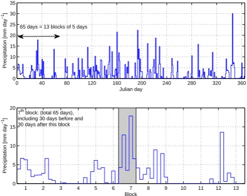
The sampling variability of the 17-year means may introduce a systematic effect in the precipitation related results. In this study we employed a length of 65 days to calculate the statis-tics for. This length is chosen for several reasons:

1. Leander and Buishand (2007) selected 65 days to reduce the sampling variability based on a study by Shabalova et al. (2003), in which HadRM2 precipitation was cor-rected for a hydrological application to the Rhine basin. Shabalova et al. (2003) state that the sampling variabil-ity is reduced using a 70-day window;

2. The block length cannot be chosen to be too small, because then one would be correcting for differences which are caused by natural variability instead of cor-recting for systematic model errors;

3. A sensitivity analysis for block lengths of 25, 35, 45, 65, 85 and 105 days revealed that block lengths of 25, 35 and 45 days improved corrections during Septem-ber/October, but lead to worse results for July/August. Block lengths of 85 and 105 days resulted in worse per-formance for nearly all months (Fig. 2);

4. RMSE for daily precipitation differences were smaller for 65-day block lengths than for lengths of 25, 35 and 45 days (Fig. 2);

Thus, in this study we determined the parameters a and b

for every five-day period of the year, including data from all years available, in a window including 30 days before and after the considered five-day period. The determination of theb parameter is done iteratively. It was determined such that the CV of the corrected daily precipitation matches the CV of the observed daily precipitation. In this way, the CV is only a function of parameterbaccording to:

(5)

J F M A M J J A S O N D 50

60 70 80 90 100 110 120

Month

Precipitation [mm]

obs era 25 35 45 65 85 105

J F M A M J J A S O N D 0.35

0.4 0.45 0.5 0.55 0.6

Month

[image:5.595.307.549.63.254.2]

RMSE [mm]

Fig. 2. Left: Average monthly precipitation sums for various block lengths. “obs” denotes the observed precipitation, while “era” de-notes the uncorrected ERA15/REMO precipitation. The sensitivi-ties are shown for block lengths of 25, 35, 45, 65, 85 and 105 days. Right: RMSEs of daily precipitation differences for various block lengths.

in whichP is the precipitation in a block of 65 days times 17 years. With the determined parameterb, the transformed daily precipitation values are calculated using:

P∗=Pb (6)

The parameter a is then determined such that the mean of the transformed daily values corresponds with the observed mean. The resulting parameteradepends onb. At the end, each block of 5 days has its owna andb parameter, which are assumed to be the same for each year. The bias correc-tion for the ERA15/REMO data set needs to be calculated for the period 1979–1995, which has a total length of 17 years. Figure 3 illustrates the division of a year into 73 blocks of 5 days. For every 5-day block, a different set ofaandb param-eters is determined using the method described above. The top panel of Fig. 3 represents the daily precipitation through-out the year. The bottom panel zooms in to the first 65 days of the year resulting in 13 blocks of 5 days each. Parameters of block 7 are calculated using 30 days before and 30 days after the considered block, and taking into account all years for which the bias correction is applied. This results in 1105 (=17×65) values for the calculation of the CV and the mean.

3.3 Temperature

Temperature cannot be corrected using a similar power law as was used for correcting precipitation, because temperature is known to be approximately normally distributed. Correct-ing a normally distributed data set with a power law function results in a data set which is not normally distributed. There-fore we used a different technique for correcting tempera-ture. The correction of temperature only involves shifting and scaling to adjust the mean and variance (Leander and

0 40 80 120 160 200 240 280 320 360

0 5 10 15 20 25 30 35

Julian day

Precipitation [mm day

−1

]

1 2 3 4 5 6 7 8 9 10 11 12 13

0 5 10 15 20

Block

Precipitation [mm day

−1

]

65 days = 13 blocks of 5 days

7th_{block: (total 65 days),}

including 30 days before and 30 days after this block

Fig. 3. Schematisation of the division of a year into 73 blocks of 5 days each for which theaandbparameters are determined. Top: daily precipitation throughout the year; Bottom: first 65 days of the year resulting in 13 blocks of 5 days each.

Buishand, 2007). For each sub-basin, the corrected daily temperatureT∗was obtained as:

T∗=Tobs+

σ (Tobs)

σ (Tera)

(Tera−Tobs)+(Tobs−Tera) (7)

where Tera is the uncorrected daily temperature from

ERA15/REMO and Tobs is the observed daily temperature

from the CHR data set. In this equation an overbar denotes the average over the considered period and σ the standard deviation. This method was not appropriate for precipitation because it may cause negative values. Again both statistics were determined for each 5-day block of the year separately, using the same 65-day windows as for the bias correction of daily precipitation.

4 Results

4.1 Introduction

In the following sub-sections the data are analyzed spa-tially and temporally. We analyse how well the relevant statistics (CV, standard deviation and mean) of the corrected ERA15/REMO data match those of the observations after the bias correction has been applied. Extended analyses are done on the behaviour of extremes, fraction of wet days and lag-1 autocorrelations. This is done for precipitation and temper-ature separately. The sensitivity of the determineda andb

[image:5.595.49.288.63.224.2]

(6)

[image:6.595.306.547.58.311.2]

692 W. Terink et al.: Bias correction of downscaled precipitation and temperature reanalysis data

Fig. 4. Top: MBE for the uncorrected and corrected ERA15/REMO precipitation [mm] per sub-basin for the period 1979–1995; Bot-tom: RMSE for the uncorrected and corrected ERA15/REMO pre-cipitation [mm] per sub-basin for the period 1979–1995.

4.2 Precipitation

4.2.1 Spatial precipitation difference

The average precipitation is corrected to match the average precipitation for each window of 65 days times 17 years. It would also be of interest to know if the daily average pre-cipitation over the entire period has improved. Therefore the average daily precipitation over the period 1979–1995 has been calculated for each sub-basin separately. The average daily precipitation difference between the observations and ERA15/REMO is given by:

MBE= 1 N

N

X

i=1

Pera,i−Pobs,i (8)

where MBE is the Mean Bias Error,N the number of days,

Pera,ithe precipitation for ERA15/REMO at dayiandPobs,i

[image:6.595.48.286.59.347.2]

the precipitation for the observations at day i. The MBE for the uncorrected and corrected situation is shown in the top panel of Fig. 4 for each sub-basin separately. A pos-itive difference means that ERA15/REMO is wetter than the observed precipitation value for that specific sub-basin. As can be seen, the difference between the uncorrected ERA15/REMO and the observations varies between−2 and

Fig. 5. Top: average monthly precipitation sums [mm] for the ob-servations and the uncorrected and corrected ERA15/REMO data (solid lines). Average monthly precipitation sums +/− one stan-dard deviation are shown as well (thin lines); Bottom: scatter densi-ties for the uncorrected and corrected ERA15/REMO and observed monthly precipitation sums for each year per sub-basin.R2 coeffi-cients for the uncorrected and corrected situation are shown as well.

+2 mm d−1. The uncorrected ERA15/REMO precipitation is too wet for most of the Rhine basin, especially in the Alps and in areas close to where the river Rhine is located. From the top right panel of Fig. 4, it can be concluded that the bias correction leads to satisfactory results. Differences between the corrected ERA15/REMO and the observations have decreased notably. The spatial variation in the spread of daily precipitation differences per sub-basin is quantified by the root-mean-square-error (RMSE) of the daily precipita-tion difference between ERA15/REMO and the observaprecipita-tions (bottom panel, Fig. 4) and is given by:

RMSE=

v u u t 1

N

X

i=1

Pera,i−Pobs,i2 (9)

(7)

4.2.2 Temporal precipitation difference

The Rhine basin is subject to a strong seasonal pattern in which wet winters and dry summers are quite common. This aspect is important for the correct timing of flood peaks. Therefore, we are interested to evaluate how well the bias-corrected ERA15/REMO precipitation performs temporally. We already noticed that the daily average over the entire pe-riod has improved considerably (top panel Fig. 4). However, it is certainly possible that the average monthly precipitation sums of the corrected ERA15/REMO data differ from those of the observations, although the average ERA15/REMO precipitation over the entire period is unbiased. Average monthly precipitation sums for the observations and the un-corrected and un-corrected ERA15/REMO data are shown in the top plot of Fig. 5. Averages are calculated as weighted (based on sub-basin size) averages over the period 1979– 1995. Large differences between the observations and the un-corrected ERA15/REMO can be seen during May, June, July, September and October. However, the bias correction seems to correct for this bias reasonably well. It seems that the cor-rection method is less capable of correcting the monthly pre-cipitation sums during February, April and November. How-ever, the method was developed to correct for the mean and CV for blocks of 65 days, in which the determined 5-daya

andb parameters will have an effect on the statistics of the neighbouring and partly overlapping 65-day blocks. There-fore, it may happen that average monthly precipitation sums of the uncorrected ERA15/REMO data match those of the observations better than the corrected ERA15/REMO data does.

It can be noticed that precipitation is corrected from a wet to a drier situation for almost the entire year. Consid-ering Fig. 5, the wet bias is especially large during sum-mer. According to Frei et al. (2003), who studied precipi-tation statistics for the European Alps, wind field deforma-tion and deflecdeforma-tion of hydrometeors over the gauge orifice results in a systematic measurement bias. Estimates of this error for the Alpine region are largest in winter (high wind speed, high fraction of snowfall), when the undercatch is about 8% for gauges below 600 m above sea level. For sum-mer the undercatch varies between 4% at low and 12% at high-altitude stations. Therefore the large wet bias during summer could partly be a result of a systematic undercatch in the rain gauges. However, the undercatch is relatively small (only 4%) for the largest part of the Rhine basin during sum-mer. Instead of individual rain gauges, we used sub-basin averaged precipitation values, which are calculated using ad-vanced interpolation techniques in which orography and ori-entation of the terrain are taken into account (see Sect. 2). Based on this we assume that the effect of overcorrecting for undercatch is minimal.

In September and October the correction is the other way around, and according to the top plot of Fig. 5 the described method has some difficulties in correcting for this shift. This

suggests that the employed method is less capable of correct-ing the precipitation sum if the observed precipitation and ERA15/REMO precipitation show an opposite signal. This minimum for ERA15/REMO precipitation in September and October was also found by Kotlarski et al. (2005). They com-pared 3 reference data sets with downscaled ERA15, using 4 different RCMs. Kotlarski et al. (2005) found an overesti-mation of precipitation in REMO in June and subsequently a strong decrease of mean monthly rainfall until September. This is probably connected to the annual cycle of vegeta-tion characteristics implemented in this model, which causes strong evaporation in early summer and consequently a rapid decline of soil water storage. In late summer, the dry soil pre-vents evaporation and therefore local water supply for the at-mosphere, resulting in a decrease of precipitation. This late-summer drying problem was also found by Hagemann and Jacob (2007), who used an ensemble of 10 RCMs to conduct climate simulations for current and future climate conditions. A late-summer drying problem was found for all RCMs over Central Europe and is a common feature in several RCMs.

The correction method applied in this study uses the same

aandbparameters for each year. We noticed that the correc-tion method performs quite well when considering the aver-age monthly precipitation sums. It remains to be seen how well the method performs when considering individual years. To answer this question, the average monthly precipitation sum plus and minus one standard deviation has been plot-ted as well (thin lines). Considering these results it seems that the correction method works quite well for the months May until October, but for November until April there are three years in which the uncorrected data matches the ob-servations better than the corrected data does. To consider both the monthly performance for each year and the per-formance per sub-basin, the bottom plots of Fig. 5 repre-sent the relation between the observed and ERA15/REMO monthly precipitation sums for each year per sub-basin, both for the uncorrected (left plot) and corrected (right plot) sit-uation in a scatter density plot. It can be noticed that the monthly precipitation sums for the corrected situation match those of the observations better than those of the uncorrected situation. Based on these results we conclude that the over-all performance of the ERA15/REMO precipitation has im-proved, although there are a few years for which the uncor-rected ERA15/REMO precipitation performs better.

4.2.3 Variation and sensitivity of parameters

The determinedaandbparameters affect the corrected daily precipitation value. It is of major importance how sensitive these parameters are to the period for which they were deter-mined. What would happen with the parameters if we had selected a different time period for determing the parame-ters? The two left panels of Fig. 6 show boxplots for thea

(8)

0 50 100 150 200 250 300 350

0.5 1 1.5 2 Parameter a Julian day Boxplot parameter a

Mean: 0.78

0 0.5 1 1.5 2 2.5 3

0 0.5 1 1.5 2 2.5 3 3.5

Histogram parameter a

Mean: 1.09 Std: 0.36

Parameter a

Frequency

0 50 100 150 200 250 300 350

0.8 1 1.2 1.4 1.6 Parameter b Julian day Boxplot parameter b

Mean: 1.16

0 0.5 1 1.5 2 2.5 3

0 1 2 3 4 5 6 7 8

Histogram parameter b

Mean: 1.07 Std: 0.14

Parameter b

Frequency

x 104

0 50 100 150 200 250 300 350

Mean: 0.78

0 0.5 1 1.5 2 2.5 3

0 0.5 1 1.5 2 2.5 3 3.5

Mean: 1.09 Std: 0.36

Parameter a

Frequency

0 50 100 150 200 250 300 350

Mean: 1.16

0 0.5 1 1.5 2 2.5 3

0 1 2 3 4 5 6 7 8

Mean: 1.07 Std: 0.14

Parameter b

Frequency

x 104

0 50 100 150 200 250 300 350

Mean: 0.78

0 0.5 1 1.5 2 2.5 3

0 0.5 1 1.5 2 2.5 3 3.5

Mean: 1.09 Std: 0.36

Parameter a

Frequency

0 50 100 150 200 250 300 350

Mean: 1.16

0 0.5 1 1.5 2 2.5 3

0 1 2 3 4 5 6 7 8

Mean: 1.07 Std: 0.14

Parameter b

Frequency

x 104

0 50 100 150 200 250 300 350

Mean: 0.78

0 0.5 1 1.5 2 2.5 3

0 0.5 1 1.5 2 2.5 3 3.5

Mean: 1.09 Std: 0.36

Parameter a

Frequency

0 50 100 150 200 250 300 350

Mean: 1.16

0 0.5 1 1.5 2 2.5 3

0 1 2 3 4 5 6 7 8

Mean: 1.07 Std: 0.14

Parameter b

Frequency

x 104

[image:8.595.83.511.62.428.2]

x 104

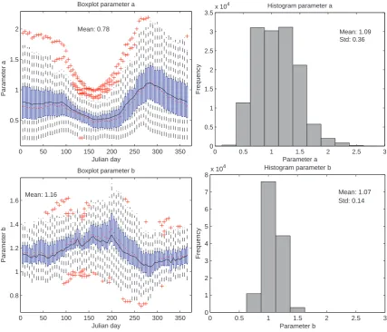
Fig. 6. Top left: boxplot for parameterafor each block of 5 days. The boxplot is calculated taking into account the values from all

sub-basins. Median values are represented with the horizontal red lines. Area-weighted average parameter values are shown with the black solid line. Outliers (red crosses) are calculated as values larger than 1.5 times the interquartile range. Top right: histogram of bootstrap values for parameterafor 1000 random samples of 65 days from 17 years of data. Samples are taken from each of the sub-basins and from block 55, including 30 days before and after this block. Bottom left: boxplot for parameterb. Bottom right: histogram of bootstrap values for parameterbfor block 55.

values from all sub-basins. Outliers are defined as values larger than 1.5 times the interquartile range and are indicated with red crosses. It is clear that parametera is smaller than one during almost the entire year. Parametera was deter-mined to fit the mean of ERA15/REMO with that of the ob-servations. It can be concluded that the average precipitation has to be corrected from a wet to a drier situation for almost the entire year. This correction is especially large during summer, as was already noticed from Fig. 5. However, the spread in thea-parameter is smallest during summer. This spread is large during winter, which implies a large variation in thea-parameter for the various sub-basins. It could be that the uncertainty of thea-parameter is large during winter. Outliers indicate sub-basins, especially during the first 280 days of the year, for which thea-parameter is substantially

larger or smaller than for most of the sub-basins. Sub-basin 1 (see Fig. 1) is an outlier during almost the entire year. Sub-basin 119 (eastern part of Switzerland) has ana-parameter which is smaller than 1.5 times its interquartile range for the 26th and 27th block. The spread in theb-parameter (Fig. 6 bottom left panel) is smaller than was the case for parameter

a. Outliers can be found throughout the entire year, except for the first 55 days of the year. Large outliers forb occur mainly in sub-basin 107. Small outliers forb occur mainly for sub-basin 1. Parameterbis larger than one during almost the entire year. The CV has to be corrected most during the summer months.

To address the uncertainty concerning the determineda

(9)

spread in botha andbis quite large. We took 1000 random samples of 65 days from the 17 years of data available for block 55, and determined for each sample a newaandb pa-rameter. The bootstrapping procedure is performed for each of the sub-basins individually. The results of this analysis are shown in the two histograms of Fig. 6. It can be concluded that the uncertainty range for parametera is larger than for parameterb. In other words, the largest uncertainty is asso-ciated with correcting the mean of the precipitation values.

4.2.4 Statistics

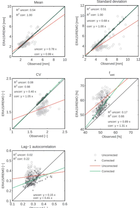
In Sect. 3 we described the method of the bias correction, that is employed to fit the mean and CV for the precipitation data. Figure 7 shows several scatter plots for the fitting statistics as well as for the fraction of wet days (fwet) and the

lag-1 autocorrelations. These statistics are calculated for each of the sub-basins separately, resulting in 134 data points for each graph. The observed statistics are plotted versus those of the uncorrected and corrected ERA15/REMO data.

Of course the mean, standard deviation and CV of the ob-servations match those of the corrected ERA15/REMO al-most perfectly, because those were the fitting criteria. In-terestingly, also the correlation between the fraction of wet days in the observations and in ERA15/REMO has improved significantly for the corrected ERA15/REMO data. Also the lag-1 autocorrelations of the corrected ERA15/REMO data match those of the observations better than those of the un-corrected ERA15/REMO data. These results can be consid-ered as good, because the method of bias correction applied in this study was only intended to correct for the CV and mean, not for the fraction of wet days or the lag-1 autocorre-lation.

For climate impact studies it is important that the hydro-logical model is capable of simulating the runoff generated by large multi-day precipitation events well enough. These large multi-day precipitation events often result in floods. Therefore, we have selected all 10-day precipitation sums during winter. The non-exceedance probabilities for these 10-day precipitation sums have been investigated in Fig. 8. According to Furrer and Katz (2008) a Generalized Pareto distribution is capable of fitting high intensity precipitation data. Therefore we have fitted a Generalized Pareto distri-bution through the data. The Generalized Pareto distridistri-bution function is given by:

y=f (x|k,σ,θ )=1 σ

1+kx−θ σ

−1−1 k

(10) wherekis the shape parameter,σ is the scale parameter and

θ is the threshold parameter. Only the fit to the observed 10-day precipitation sums is shown, because the other two fits are similar. All parameters are estimated using the max-imum likelihood method (Aldrich, 1997). Both the uncor-rected and coruncor-rected ERA15/REMO data match the obser-vations well for non-exceedance probabilities smaller than

2 4 6 8 10

0 2 4 6 8 10

R2 uncorr: 0.54

R2_{corr: 1.00}

uncorr: y = 0.78 x corr: y = 0.99 x

Observed [mm]

ERA15/REMO [mm]

Mean

2 4 6 8 10 12

R2 uncorr: 0.51

R2_{corr: 1.00}

uncorr: y = 0.68 x

corr: y = 1.00 x

Observed [mm]

ERA15/REMO [mm]

Standard deviation

1 1.5 2 2.5

R2_{uncorr: 0.08}

R2_{corr: 0.98}

Observed [−]

ERA15/REMO [−]

CV

40 50 60 70

R2_{uncorr: 0.17}

R2 corr: 0.66

Observed [%]

ERA15/REMO [%]

f

wet

0.1 0.2 0.3 0.4 0.5 0.6 0.1 0.2 0.3 0.4 0.5 0.6

R2_{uncorr: 0.02}

R2 corr: 0.22

Observed [−] ERA15/REMO [−] Lag−1 autocorrelation Uncorrected Corrected Uncorrected Corrected

2 4 6 8 10

0 2 4 6 8 10

R2_{uncorr: 0.54}

R2_{corr: 1.00}

Observed [mm]

ERA15/REMO [mm]

Mean

2 4 6 8 10 12

R2_{uncorr: 0.51}

R2_{corr: 1.00}

uncorr: y = 0.68 x

corr: y = 1.00 x

Observed [mm]

ERA15/REMO [mm]

Standard deviation

1 1.5 2 2.5

R2_{uncorr: 0.08}

R2_{corr: 0.98}

Observed [−]

ERA15/REMO [−]

CV

40 50 60 70

R2 uncorr: 0.17

R2 corr: 0.66

Observed [%]

ERA15/REMO [%]

f_wet

0.1 0.2 0.3 0.4 0.5 0.6 0.1 0.2 0.3 0.4 0.5 0.6

R2_{uncorr: 0.02}

R2_{corr: 0.22}

Observed [−] ERA15/REMO [−] Lag−1 autocorrelation Uncorrected Corrected Uncorrected Corrected

Fig. 7. Scatter plots of the statistics of the observed precipita-tion versus the corrected and uncorrected ERA15/REMO precipi-tation. The statistics are calculated for each sub-basin over the pe-riod 1979–1995. The fraction of wet days (fwet) is the percentage of days whereP >0.3 mm. In each subplot the square of the cor-relation coefficient (R2) and slope of the linear regression line are plotted. The black line represents thex=yline.

0.95. However, for non-exceedance probabilities larger than 0.95 the uncorrected ERA15/REMO matches the 10-day pre-cipitation sums of the observations better than the corrected ERA15/REMO does. These differences are, however, quite small. More important is that the distribution of the 10-day precipitation sums is not substantially disturbed by applying a bias correction.

4.3 Temperature

4.3.1 Spatial temperature difference

[image:9.595.311.541.63.405.2]

(10)

0 50 100 150

0 0.1 0.2 0.3 0.4 0.5 0.6 0.7 0.8 0.9 1

10−day precipitation sum [mm]

non−exceedance probability [−]

Observations

[image:10.595.305.549.63.255.2]

Uncorrected Corrected

Fig. 8. Non-exceedance probabilities of 10-day winter precipitation sums for the period 1979–1995. The 10-day precipitation sums are area-weighted averages.

Fig. 9. Top: MBE for the uncorrected and corrected ERA15/REMO temperature [◦C] per sub-basin for the period 1979–1995. Bot-tom: RMSE for the uncorrected and corrected ERA15/REMO tem-perature [◦C] per sub-basin for the period 1979–1995.

in MBE vary between−1.5 and +3.5◦C for the uncorrected ERA15/REMO data. The MBE is positive for the largest part of the Rhine basin, which means that the uncorrected

J F M A M J J A S O N D

−5 0 5 10 15 20

Month

Temperature [

°

C]

Observed

Uncorrected

[image:10.595.47.288.63.254.2]

Corrected

Fig. 10. Area-weighted monthly temperature [◦C] over the entire

Rhine basin for the period 1979–1995. Results are shown for the observations and the uncorrected and corrected ERA15/REMO.

ERA15/REMO is warmer than the observations for that part of the Rhine basin. The top right panel of Fig. 9 shows the differences between both data sets after the correction has been applied. It can be concluded that the bias correction for temperature leads to good results. Differences have de-creased substantially to values between−0.4 and +0.4◦_C. Another point of interest is the spatial variation in the spread of daily temperature differences per sub-basin. This is quan-tified by the RMSE of the daily temperature difference be-tween ERA15/REMO and the observations (Fig. 9, bottom panel). In the uncorrected situation the RMSE is quite large for some sub-basins. However, the RMSE for the corrected temperature has decreased significantly. Based on these re-sults it can be concluded that the applied correction method adjusts the daily temperature values very well.

4.3.2 Temporal temperature difference

Average monthly temperatures for the period 1979–1995 are shown in Fig. 10. Averages are calculated as area-weighted averages over the entire Rhine basin. With the bias correction we hope to capture the seasonal pattern of temperature. It can be concluded that the bias correction for temperature leads to satisfactory results. The bias-corrected ERA15/REMO tem-perature matches the observed temtem-perature almost perfectly for each month. Corrections are largest during the summer months and smallest during winter. This is mainly caused by the difference in mean temperature as shown later in Fig. 11.

4.3.3 Standard deviation and mean

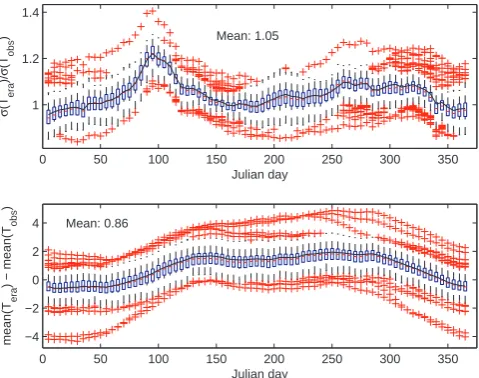
[image:10.595.47.287.316.602.2]

(11)

0 50 100 150 200 250 300 350 1 1.2 1.4 σ (Tera )/ σ (Tobs ) Julian day Mean: 1.05

0 50 100 150 200 250 300 350

−4 −2 0 2 4 mean(T era

) − mean(T

obs

)

[image:11.595.48.288.62.251.2]

Julian day Mean: 0.86

Fig. 11. Top: boxplot for the ratios of the ERA15/REMO standard deviations over the observed standard deviations. Bottom: boxplot for the differences between the ERA15/REMO average tempera-tures and observed average temperatempera-tures. Boxplots are shown for each block of 5 days, where each box represents the spread between all sub-basins. Area-weighted averages for each block of 5 days are represented with the solid black line. Median values are represented with the horizontal red lines while outliers are indicated with the red crosses and are calculated as values larger than 1.5 times the interquartile range.

it is interesting to know how the ratio of the ERA15/REMO standard deviation over the observed standard deviation for temperature varies during the year. The spread in ratios for all sub-basins, before the correction is applied, is represented in the boxplot of Fig. 11 (top panel). A seasonal pattern can be distinguished from this figure. From January on, there is an upward trend until the start of summer, which suggests an increasing variation in temperature for ERA15/REMO when approaching summer. During summer this ratio again ap-proaches one, suggesting a similar standard deviation for the observed and ERA15/REMO temperature. Around mid-summer this ratio is increasing again, resulting in a larger spread in temperature for ERA15/REMO during this period. The area-weighted average ratio of 1.05 suggests that the average spread in temperature for ERA15/REMO is larger than that for the observations. The bottom panel of Fig. 11 represents the spread in average temperature differences be-tween the ERA15/REMO (Tera) and observed temperature

(Tobs). Especially during summer the difference between

TeraandTobstends to be larger, suggesting a much warmer

17-year average for ERA15/REMO than for the observations. The 17-year average temperature appears to be warmer for ERA15/REMO throughout the entire year for almost all sub-basins. The overal area-weighted average temperature dif-ference of 0.86◦C suggests that the average temperature for ERA15/REMO is larger than that for the observations.

0 2 4 6 8 10 12 0 2 4 6 8 10 12

R2_{uncorr: 0.77}

R2 corr: 1.00

Observed [°C]

ERA15/REMO [

°

C]

Mean

5 6 7 8 9 10

R2_{uncorr: 0.30}

R2_{corr: 0.99}

uncorr: y = 0.52 x

corr: y = 1.07 x

Observed [°C]

ERA15/REMO [

°

C]

Standard deviation

0 2 4 6

R2_{uncorr: 0.85}

R2_{corr: 0.99}

Observed [−]

ERA15/REMO [−]

CV

0.9 0.92 0.94 0.96 0.98 0.9

0.92 0.94 0.96 0.98

R2_{uncorr: 0.17}

R2_{corr: 0.44}

Observed [−]

ERA15/REMO [−]

Lag−1 autocorrelation

Uncorrected Corrected Uncorrected Corrected 0 2 4 6 8 10 12

0 2 4 6 8 10 12

R2_{uncorr: 0.77}

R2 corr: 1.00

Observed [°C]

ERA15/REMO [

°

C]

Mean

5 6 7 8 9 10

R2_{uncorr: 0.30}

R2_{corr: 0.99}

Observed [°C]

ERA15/REMO [

°

C]

Standard deviation

0 2 4 6

R2_{uncorr: 0.85}

R2_{corr: 0.99}

Observed [−]

ERA15/REMO [−]

CV

0.9 0.92 0.94 0.96 0.98 0.9

0.92 0.94 0.96 0.98

R2_{uncorr: 0.17}

R2_{corr: 0.44}

Observed [−]

ERA15/REMO [−]

Uncorrected Corrected Uncorrected Corrected

0 2 4 6 8 10 12

R2 uncorr: 0.77

R2_{corr: 1.00}

Observed [°C]

ERA15/REMO [

°

C]

5 6 7 8 9 10

R2_{uncorr: 0.30}

R2 corr: 0.99

Observed [°C]

ERA15/REMO [

°

C]

0 2 4 6

R2_{uncorr: 0.85}

R2 corr: 0.99

Observed [−]

ERA15/REMO [−]

CV

0.9 0.92 0.94 0.96 0.98

R2_{uncorr: 0.17}

R2 corr: 0.44

Observed [−]

ERA15/REMO [−]

Uncorrected Corrected Uncorrected Corrected

Fig. 12. Scatter plots of the statistics of the observed ture versus the corrected and uncorrected ERA15/REMO tempera-ture. The statistics are calculated for each sub-basin over the period 1979–1995. In each subplot the square of the correlation coefficient (R2) and slope of the linear regression line are plotted. The black line represents thex=yline.

4.3.4 Statistics

The most important statistics for the uncorrected and cor-rected ERA15/REMO temperature are plotted against those of the observations in Fig. 12. The considered statistics are the mean, standard deviation, CV and lag-1 autocorrelation. They are calculated over the entire period 1979–1995, for each sub-basin separately. As mentioned before, the cho-sen method of bias correction only corrects for the mean and the standard deviation. This is clearly visible in the plots of the mean, standard deviation and CV, where the cor-rected ERA15/REMO statistics are almost equal to those of the observations. Despite the fact that the correlation coeffi-cients between the lag-1 autocorrelations for ERA15/REMO and the observations have increased for the corrected situ-ation, the points have moved further away from the x=y

line. However, considering the scale of the y-axis, this result seems to be of minor importance.

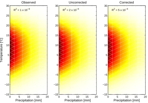
4.4 Relation between precipitation and temperature

[image:11.595.311.544.63.285.2]

(12)

0 5 10 15 20

−15 −10 −5 0 5 10 15 20 25 30

Observed

Precipitation [mm]

Temperature [

°

C]

R2_{= 1 x 10}−4

0 5 10 15 20

−15 −10 −5 0 5 10 15 20 25 30

Uncorrected

Precipitation [mm]

R2_{= 2 x 10}−4

0 5 10 15 20

−15 −10 −5 0 5 10 15 20 25 30

Corrected

Precipitation [mm]

[image:12.595.47.289.62.231.2]

R2_{= 5 x 10}−4

Fig. 13. Dependency between the daily precipitation and tempera-ture of the observed and uncorrected and corrected ERA15/REMO data for the period 1979–1995. The squared correlation coefficient for the correlation between precipitation and temperature is shown as well.

sub-basins. Results are shown for the observations and the uncorrected and corrected ERA15/REMO data. The ex-tremely lowR2for the correlation between precipitation and temperature indicates the absence of correlation. From this figure we can conclude that the pattern of points and corre-lation coefficient are not drastically disturbed after the bias correction is applied. This result is robust on a seasonal level as well.

4.5 Validation

4.5.1 Introduction

The previous analysis focused on the bias correction for the entire period 1979–1995. In climate impact studies, the bias correction parameters are often determined for a certain ref-erence period, and subsequently applied to a future climate period. Therefore we have selected 10 years from the pe-riod 1979–1995 as a calibration pepe-riod for determining the correction parameters, and applied the determined correction parameters for the remaining 7 years, known as the validation period. With this we want to evaluate how well the method of Leander and Buishand (2007) is capable of correcting an-other period for which the parameters were not determined. This analysis is split into two parts, wherein the first part uses the period 1979–1988 as the calibration period and the period 1989–1995 as the validation period. The second ana-lysis takes 100 samples, in which each sample consists of 10 randomly chosen years from the period 1979–1995 which are used for calibration and the remaining 7 years are used for validation. With this analysis we want to quantify the un-certainty associated with the selection of 10 calibration and 7 validation years.

Fig. 14. Top: MBE for the uncorrected and corrected

ERA15/REMO precipitation [mm] per sub-basin for the validation period 1989–1995. Bottom: RMSE for the uncorrected and cor-rected ERA15/REMO precipitation [mm] per sub-basin for the val-idation period 1989–1995.

4.5.2 Continuous period

The previously described bias correction method has been applied to determine the correction parameters for the pe-riod 1979–1988. These parameters have been used to cor-rect precipitation and temperature for the period 1989–1995. Similar to Fig. 4, the MBE for the uncorrected and corrected ERA15/REMO precipitation per sub-basin are shown in the top panel of Fig. 14 for the validation period 1989–1995. Spatial precipitation differences have been minimized for the corrected situation, although less notable than for the analy-sis for the entire period 1979–1995. We already noticed that the RMSE between the observed and ERA15/REMO precipi-tation was not improved for the corrected situation when con-sidering the entire period 1979–1995. Looking at the valida-tion period (bottom panel Fig. 14), it seems that the RMSE even increases for the corrected situation. This may result in worse performance of a hydrological model, if the parame-ters were used to correct a meteorological forcing dataset for a period for which the parameters were not determined.

[image:12.595.307.547.62.337.2]

(13)

[image:13.595.46.288.59.310.2]

Fig. 15. Top: average monthly precipitation sums [mm] for the observations and the uncorrected and corrected ERA15/REMO data for the validation periond 1989–1995 (solid lines). Average monthly precipitation sums +/- one standard deviation are shown as well (thin lines). Bottom: scatter densities for the uncorrected and corrected ERA15/REMO and observed yearly monthly precipi-tation sums per sub-basin for the validation periond 1989–1995.R2 coefficients for the uncorrected and corrected situation are shown as well.

March, April, August and September. Considering the stan-dard deviations, it seems that especially for March and September there are some years for which the correction is too wet. Similar to Fig. 5, the monthly precipitation sums for each separate year and individual sub-basin are plotted in the scatter density plots of Fig. 15 (bottom panel) for the uncorrected and corrected situation for the validation period. Considering theR2 coefficients, we can see an overal im-provement, although less important than for the entire cali-bration period 1979–1995. Based on these results we con-clude that the determined correction parameters are able to correct ERA15/REMO precipitation in a validation period during the warmer summer months, but that the uncorrected precipitation is closer to the observations for most winter months and especially for March and September.

The MBE for the uncorrected and corrected ERA15/REMO temperature per sub-basin are shown in the top panel of Fig. 16 for the validation period. It appears that the determined parameters for the calibration period 1979–1988 work very well for the validation period, too. Also the RMSE between the daily ERA15/REMO tempera-ture and observed temperatempera-ture is minimized, meaning that the daily temperature values are corrected for the validation period as well (bottom panel Fig. 16).

Fig. 16. Top: MBE for the uncorrected and corrected

ERA15/REMO temperature [◦C] per sub-basin for the validation period 1989–1995. Bottom: RMSE for the uncorrected and cor-rected ERA15/REMO temperature [◦C] per sub-basin for the vali-dation period 1989–1995.

J F M A M J J A S O N D

0 2 4 6 8 10 12 14 16 18 20

Month

Temperature [

°

C]

Observed Uncorrected

Corrected

Fig. 17. Area-weighted monthly temperature [◦C] over the

[image:13.595.306.546.61.350.2] [image:13.595.307.549.433.626.2]

(14)

−0.50 0 0.5

10 20 30 40 50 60 70

Calibration period − uncorrected

Mean: 0.08 Std: 0.05

Frequency

−0.50 0 0.5

10 20 30 40 50 60 70

Calibration period − corrected

Mean: 0.00 Std: 0.02

−0.50 0 0.5

5 10 15 20 25

Validation period − uncorrected

Mean: 0.07 Std: 0.07

Precipitation difference [mm]

Frequency

−0.50 0 0.5

5 10 15 20 25

Validation period − corrected

Mean: 0.02 Std: 0.16

[image:14.595.306.549.61.327.2]

Precipitation difference [mm]

Fig. 18. Top: histograms of 100 samples of average daily precipi-tation differences between the uncorrected and observed (left), and between the corrected and observed precipitation (right) for the cal-ibration period. Bottom: similar, but for the validation period.

Monthly temperature averages for the validation period are shown in Fig. 17. The correction parameters for temperature adjust the average monthly temperatures very well for the validation period, except for the months November, Decem-ber, January and February.

4.6 Random sampling

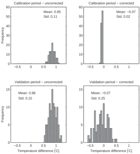
For this analysis we took 100 random samples of 10 years from the 17 years available, and used these years to deter-mine the correction parameters. The deterdeter-mined parame-ters have been used to correct the ERA15/REMO data for the remaining 7 years, denoted as the validation period. For each validation sample we calculated the average daily pre-cipitation and temperature value, averaged over the entire Rhine basin. The differences between the uncorrected and observed, and the corrected and observed values are taken as a measure of how well the method performs for a ran-domly chosen period for calibration and validation. The re-sults of this analysis are shown in the histograms of Fig. 18 and Fig. 19 for precipitation and temperature, respectively. It is clear that for the majority of samples for the calibration pe-riod the precipitation difference is smaller for the corrected situation. For the validation period it turns out that for the corrected situation the spread in precipitation differences in-creases, but that the overal average has improved. The total absolute differences for the 100 samples are 7.99, 2.01, 8.13

−0.5 0 0.5 1 0

10 20 30 40 50 60

Calibration period − uncorrected

Mean: 0.85 Std: 0.11

Frequency

−0.5 0 0.5 1 0

10 20 30 40 50 60

Calibration period − corrected

Mean: −0.07 Std: 0.02

−0.5 0 0.5 1 0

5 10 15

Validation period − uncorrected

Mean: 0.86 Std: 0.15

Temperature difference [°C]

Frequency

−0.5 0 0.5 1 0

5 10 15

Validation period − corrected

Mean: −0.07 Std: 0.25

[image:14.595.47.289.62.319.2]

Temperature difference [°C]

Fig. 19. Top: histograms of 100 samples of average daily temper-ature differences between the uncorrected and observed (left), and between the corrected and observed temperature (right) for the cal-ibration period. Bottom: similar, but for the validation period.

and 13.04 mm for the uncorrected and corrected precipitation during the calibration period, and uncorrected and corrected precipitation during the validation period, respectively. It is not clear what causes this large spread in precipitation dif-ference for the validated corrected precipitation. A possible explanation could be some low frequency components in the rainfall series. This is not further investigated as such in this paper. We expect that larger sample sizes (in excess of 10 years) lead to a decrease in the spread of precipitation biases. Therefore, it is recommended to use as many years as possi-ble to have the largest sample size for determining the correc-tion parameters. Results for temperature look more promis-ing. Large frequencies are now found to be centered around zero temperature difference for the validated corrected tem-perature.

5 Conclusions and perspectives

5.1 Conclusions

(15)

determined for a calibration period. The most important re-sults are:

1. Precipitation and temperature for the uncorrected ERA15/REMO were found to be too wet and too warm for most of the Rhine basin;

2. Precipitation and temperature are corrected very well for the calibration period 1979–1995;

3. The RMSE of the daily precipitation difference between the ERA15/REMO and observed precipitation is not smaller for the corrected precipitation values;

4. The correction method also seems to improve the frac-tion of wet days for precipitafrac-tion and lag-1 autocorrela-tions for precipitation and temperature;

5. Bootstrapping for the parametersa andbshowed that the uncertainty is largest in correcting for the mean and the spread for these parameters is largest during winter; 6. Determined correction parameters for the period 1979– 1988 are able to correct precipitation and temperature for the period 1989–1995. Precipitation correction dur-ing the validation period works well, especially for May, June, July and October. However, the validation re-sults in over-adjustment of the monthly precipitation in March and September;

7. The RMSE has increased for the corrected ERA15/REMO precipitation during the validation period. This is mainly due to the over-adjustment of precipitation in March and September;

8. When taking random years for calibration, the spread in MBE between ERA15/REMO and the observations has increased for the corrected situation during the val-idation period. However, the overal average MBE has decreased for the corrected precipitation during the val-idation period;

9. Temperature is corrected in a satisfactory manner for the randomly selected years used as validation period;

5.2 Perspectives

In Hurkmans et al. (2010) we use the bias-corrected precipi-tation and temperature to calibrate VIC and do a climate im-pact study. VIC, however, needs other meteorological forc-ing data as well, such as wind speed, incomforc-ing short- and longwave radiation, vapour pressure and specific humidity. Correcting precipitation and temperature only would violate the energy balance present in ERA15/REMO. Unfortunately there were no observations for the other forcing variables available at the temporal and spatial resolution used in this study and they are therefore left uncorrected. For future work this could be addressed using a multi-variate bias correction

method, in which the forcing variables are corrected preserv-ing the energy balance. Such methods are currently unknown to us and probably very time consuming. However, for cal-ibration purposes we expect precipitation and temperature to have the largest influence on the performance of the hy-drological model. Moreover, for operational purposes wa-ter managers would be more inwa-terested in probabilities than uncertainties. For a water manager the probability for e.g. a discharge exceeding a certain threshold would have more importance than the uncertainty present in RCM data and subsequently the hydrological model output. Therefore, it is very useful for ongoing research on climate impact stud-ies to address the uncertainty in the RCM and hydrological model, and translate this to the probability of e.g. the occur-rence of floods and droughts. We already mentioned that this method of bias correction can easily be applied to other river basins if enough meteorological data are available. However, the results in the current study are mainly focusing on the Rhine basin. Therefore, it is uncertain how the correction methodology performs in other river basins (with other data sets) and therefore it is not possible to define operational ap-plications. Thus, it is recommended to apply the correction method to several river basins and RCMs with several reso-lutions in order to obtain information which could be useful for operational applications.

Currently there are other existing methods for bias cor-rection available. For example Hay et al. (2002) applied a gamma transform to correct RegCM2 precipitation data. They found that the corrected precipitation data did not con-tain the day-to-day variability present in the observed data set. We have found that the correction method applied in the current study does not lead to a decrease in RMSE between simulated and observed precipitation amounts. This suggests that our method is not capable of preserving the day-to-day variability present in the observed data set either. The gamma transform is also evaluated by Piani et al. (2010). They show that the gamma transform is capable of correcting for sea-sonal means, but they do not show how the correction per-forms on a daily basis. We think the day-to-day variability is an important aspect when it comes to hydrological mod-eling, because for hydrological applications it is important that the model is capable of simulating the correct amount of streamflow at the right time and is therefore dependent on the correct timing of precipitation events. A further inter-esting experiment would be to evaluate the improvement of the hydrological model simulation with and without the bias-corrected precipitation fields, using bias-bias-corrected precipita-tion fields from various correcprecipita-tion methods (van Pelt et al., 2009; Hay et al., 2002; D´equ´e, 2007; Piani et al., 2010). This was also suggested by Piani et al. (2010).

(16)

702 W. Terink et al.: Bias correction of downscaled precipitation and temperature reanalysis data uncertainty with the selection of 10 years for calibration and

7 years for validation was quantified by taking 100 samples, in which each sample consists of 10 randomly selected years which are used for calibration and the remaining 7 years are used for validation. This resulted in the fact that the spread in MBE between ERA15/REMO and the observations in-creased for the corrected situation during the validation pe-riod. At this moment, it is not clear what causes this dif-ference for the validated corrected precipitation. A possi-ble explanation could be some low frequency components in the rainfall series. More research considering low frequency components is recommended. However, the overal average MBE has decreased for the corrected ERA15/REMO precip-itation during the validation period.

In Hurkmans et al. (2010), we apply the same bias cor-rection method to correct for the bias between a climate run of the 20st century and the observations. This results in a set of correction parameters which are different from those derived in the current study. The climate run of the 20st cen-tury is actually an ECHAM5 run which is downscaled with REMO (Jacob, 2001). The correction parameters are subse-quently applied to the future climate scenarios. These future scenarios were created by forcing the ECHAM5 model with IPCC carbon emission scenarios (A1B, A2 and B1; IPCC, 2000) and finally downscaling with REMO (Jacob, 2001). We have shown that the derived correction parameters in a calibration period are able to correct precipitation and tem-perature in a validation period. This strategy of climate im-pact assessment has been applied before by others; for exam-ple van Pelt et al. (2009) applied a bias correction to down-scaled ECHAM5 data, were ECHAM5 was downdown-scaled with RACMO2. They assessed the impact of climate change on discharge for the Meuse basin by forcing ECHAM5 with a transient (1950–2100) simulation of ECHAM5 using ob-served greenhouse gases for 1950–2000, and using the SRES A1B scenario for the 21st century. Lenderink et al. (2007) used the hydrological model Rhineflow driven by meteoro-logical data from a 90-year simulation with the HadRM3H RCM for both present-day and future climate, using the same bias correction for future climate as detected for present-day climate. In all these studies, it is assumed that the bias cor-rection parameters in the present-day climate remain invari-ate in future climinvari-ate projections. However, Christensen et al. (2008) demonstrated that it is indeed necessary to correct for a bias present in the RCM, but that the common assump-tion of bias cancellaassump-tion (invariance) in climate change pro-jections can have serious limitations when temperatures in the warmest months exceed 4–6◦_{C above present day} con-ditions. Thus correction parameters derived for the current climate cannot always be used to correct precipitation and temperature in a future climate. This study also demonstrates that the assumption of a constant model bias may not hold, because the determined correction parameters may result in over-adjustment of precipitation during the validation period. For hydrological applications this may lead to overestimation

of the observed discharges. Therefore, if possible, we should always validate the simulated discharges with observed dis-charges when it comes to hydrological modeling with bias-corrected RCM data. This would only be possible with RCM data of the current climate, because observed discharges are obviously not available for a future climate.

Acknowledgements. This research was financially supported by the European Commission through the FP6 Integrated Project NEWATER and the BSIK ACER project of the Dutch Climate Changes Spatial Planning programme. The authors would like to thank Adri Buishand (KNMI) for fruitful discussions concerning bias corrections. Daniela Jacob from the Max Planck Institut f¨ur Meteorologie in Hamburg, Germany, is kindly acknowledged for providing the downscaled reanalysis data. The international Commission for the Hydrology of the Rhine basin (CHR) is acknowledged for providing the observed precipitation and temper-ature data.

Edited by: F. Pappenberger

References

Aldrich, J.: R. A. Fisher and the Making of Maximum Likelihood 1912–1922, Stat. Sci., 12, 162–176, 1997.

Bergstr¨om, S. and Forsman, A.: Development of a conceptual de-terministic rainfall-runoff model, Nordic Hydrology, 4, 147–170, 1973.

Beven, K.: Changing ideas in hydrology – the case of physically based models, J. Hydrol., 105, 157–172, 1989.

Brandsma, T. and Buishand, T.: Rainfall generator for the Rhine basin: Multi-site generation of weather variables by nearest-neighbour resampling, KNMI Publication, 186-II, 58 pp., 1999. Christensen, J., Boberg, F., Christensen, O., and Lucas-Picher, P.:

On the need for bias correction of regional climate change pro-jections of temperature and precipitation, Geophys. Res. Lett., 35, L20709, doi:10.1029/2008GL035694, 2008.

D¨allenbach, F.: Gebietsniederschlag Schweiz: Interpolation und Berechnung der Niederschlagsdaten. Gutachten im Auftrag der Landeshydrologie und Geologie (LHG), Tech. rep., Meteotest, Bern, Switzerland., 2000.

de Wit, M. and Buishand, T.: Generator of rainfall and discharge extremes (GRADE) for the Rhine and Meuse basins, KNMI Pub-lication, 218, 2007.

de Wit, M., van den Hurk, B., Warmerdam, P., Torfs, P., Roulin, E., and van Deursen, W.: Impact of climate change on low-flows in the river Meuse, Clim. Change, 82, 351–372, doi: 10.1007/s10584-006-9195-2, 2007.

D´equ´e, M.: Frequency of precipitation and temperature extremes over France in an anthropogenic scenario: Model results and sta-tistical correction according to observed values, Global and Plan-etary Change, 57, 16–26, doi:10.1016/j.gloplacha.2006.11.030, 2007.