Sensitivity of point scale surface runoff predictions to rainfall resolution

www.hydrol-earth-syst-sci.net/11/965/2007/ © Author(s) 2007. This work is licensed under a Creative Commons License.

Earth System

Sciences

Sensitivity of point scale surface runoff predictions to rainfall

resolution

A. J. Hearman and C. Hinz

School of Earth and Geographical Sciences, The University of Western Australia, Crawley, Australia Received: 10 October 2006 – Published in Hydrol. Earth Syst. Sci. Discuss.: 17 November 2006 Revised: 13 February 2007 – Accepted: 21 February 2007 – Published: 5 March 2007

Abstract. This paper investigates the effects of using non-linear, high resolution rainfall, compared to time averaged rainfall on the triggering of hydrologic thresholds and there-fore model predictions of infiltration excess and saturation excess runoff at the point scale. The bounded random cas-cade model, parameterized to three locations in Western Aus-tralia, was used to scale rainfall intensities at various time resolutions ranging from 1.875 min to 2 h. A one dimen-sional, conceptual rainfall partitioning model was used that instantaneously partitioned water into infiltration excess, in-filtration, storage, deep drainage, saturation excess and sur-face runoff, where the fluxes into and out of the soil store were controlled by thresholds. The results of the numerical modelling were scaled by relating soil infiltration properties to soil draining properties, and in turn, relating these to av-erage storm intensities. For all soil types, we related maxi-mum infiltration capacities to average storm intensities (k∗) and were able to show where model predictions of infiltration excess were most sensitive to rainfall resolution (lnk∗=0.4) and where using time averaged rainfall data can lead to an un-der prediction of infiltration excess and an over prediction of the amount of water entering the soil (lnk∗>2) for all three rainfall locations tested. For soils susceptible to both infil-tration excess and saturation excess, total runoff sensitivity was scaled by relating drainage coefficients to average storm intensities (g∗) and parameter ranges where predicted runoff was dominated by infiltration excess or saturation excess de-pending on the resolution of rainfall data were determined (lng∗<2). Infiltration excess predicted from high resolution rainfall was short and intense, whereas saturation excess pro-duced from low resolution rainfall was more constant and less intense. This has important implications for the accuracy of current hydrological models that use time averaged rain-fall under these soil and rainrain-fall conditions and predictions of Correspondence to: C. Hinz

([email protected])

larger scale phenomena such as hillslope runoff and runon. It offers insight into how rainfall resolution can affect predicted amounts of water entering the soil and thus soil water stor-age and drainstor-age, possibly changing our understanding of the ecological functioning of the system or predictions of agri-chemical leaching. The application of this sensitivity analy-sis to different rainfall regions in Western Australia showed that locations in the tropics with higher intensity rainfalls are more likely to have differences in infiltration excess predic-tions with different rainfall resolupredic-tions and that a general un-derstanding of the prevailing rainfall conditions and the soil’s infiltration capacity can help in deciding whether high rain-fall resolutions (below 1 h) are required for accurate surface runoff predictions.

1 Introduction

Whilst Bronstert and Bardossy (2003) conclude that the use of high rainfall resolution is most important for high rain-fall events but not extreme events there is no clear sensitivity analysis as to the conditions where surface runoff predictions are most affected by rainfall resolution and to what extent dif-ferences in hillslope surface runoff predictions are the result of discrepancies in point scale surface runoff predictions or hillslope runoff transformations.

The earlier work of Woolhiser and Goodrich (1988) goes some way in addressing this issue with the construction of di-mensionless parameters in relation to kinematic equilibria of overland flow and the ratio of the infiltration depth at ponding to the mean storm depth. This study looks at Hortonian over-land flow and concentrates on the differences in peak runoff rates with the biggest differences in peak runoff rates occur-ring between constant rainfall and temporally varying rain-fall when the ratio of the infiltration depth at ponding to the mean storm depth is low and the ratio of the time to kinematic equilibrium on the overland flow plane to the mean duration of the storm set is also low.

These previous studies into the impacts of temporally varying rainfall and surface runoff predictions have concen-trated on Hortonian overland flow and do not consider dif-ferences in water able to enter the soil or surface runoff at-tributed to saturation excess. This study aims to expand on previous research a number of ways. Firstly, by looking at two different mechanisms of runoff generation, infiltration excess and saturation excess and how rainfall resolution may impact predictions of the mechanism dominating runoff gen-eration. This modelling approach not only sets out to inves-tigate differences in amounts of infiltration excess and sat-uration excess but also the dynamics, including maximum intensity, frequency and duration each surface runoff pro-cess is active throughout each storm event. Secondly, we quantify the effects of rainfall resolution on surface runoff generation and identify scaled rainfall and soil conditions in which model predictions are most sensitive to rainfall reso-lution. The scaling approach allows us to investigate a wider range of soil-storm relationships than studies based on spe-cific conditions. An application of this approach to rainfall from a number of locations is made in an attempt to illustrate how the model can be used to gain an understanding of the sensitivity of surface runoff predictions to rainfall resolution in different rainfall regions within Western Australia.

The recognition of the importance of using high resolu-tion rainfall data has lead to the use of stochastic simularesolu-tion of rainfall and analysis of the statistical properties of hydro-logical modelling. For this reason, in the last 20 years there have been many studies into the transformation of available rainfall data from one scale to another (for an overview see Lovejoy and Schertzer, 2005). All disaggregation methods are based on describing the variability at one scale in relation to the variability at another scale. One of the most prevalent and promising methods is the use of multifractal random cas-cades which are able to reproduce the statistical properties of

non-extreme rainfall events as well as extreme rainfall events (Veneziano et al., 1996, Over and Gupta, 1996, Menabde et al., 1997). In this paper we use the bounded random cas-cade approach described by Menabde and Sivapalan (2000) with three different sets of rainfall parameters from Western Australia as an illustration of a method to determine the soil-storm relationships most sensitive to rainfall resolution when predicting surface runoff and how this may change for differ-ent rainfall regions.

The results presented in this paper remain at the point scale. The authors wish to create a clear and accurate un-derstanding of the processes at the point scale and how these may be influenced by different soil-storm properties before these effects are further complicated by hillslope properties such as steepness, length and roughness. “Even at the point scale there is much that remains to be learned about how best to represent the dynamic characteristics of infiltration and surface runoff generation” (Beven, 2002, pp. 80).

Whilst using complex rainfall as input, we used a simple infiltration capacity threshold in a similar fashion to Yu et al. (1997) to determine infiltration excess. The simple in-filtration capacity threshold was chosen as Yu (1999) points out that the widely used Green-Ampt approach has been ap-plied mostly in relation to predicting runoff amounts as op-posed to runoff rates which we also wish to predict here. Yu et al. (1997) showed that at 1 min intervals infiltration rates were closely related to rainfall intensities and were “es-sentially independent of cumulative infiltration amount, fea-tures not in accord with the Green-Ampt infiltration equa-tion” (pp. 1295). Comparison of the Green-Ampt approach to a simple infiltration capacity threshold approach showed that the simple threshold outperformed the Green-Ampt ap-proach when compared to runoff data at a range of time in-tervals and storm events, as it was better able to represent runoff hydrographs and peak runoff rates (Yu, 1999). The aim of this paper is to investigate surface runoff predictions at a range of rainfall resolutions including high resolution rainfall less than 5 min and also to look at the dynamics of this predicted surface runoff. From the evidence outlined in Yu et al. (1997) and Yu (1999) we have adopted a point scale model that incorporates a single infiltration capacity.

Saturation excess is predicted using a simple, lumped pa-rameter bucket model. There are numerous examples of the use of simple lumped storage representations of surface hy-drology (Milly, 1994; Kirkby and Cox, 1995; Farmer et al., 2003; Woods, 2003; Struthers et al., 2007a, b). It is this minimalist, process based approach, as opposed to a more complicated Richards equation, that we wish to adopt in our attempts to investigate how using rainfall measured at vari-ous time scales will influence the triggering of surface runoff thresholds. Using this minimalist approach we are able to derive scaled soil-storm properties that relate a wide range of soil and storm conditions to the impact of time averaged rain-fall data on surface runoff predictions. Although these point scale saturation excess predictions have limited application

A. J. Hearman and C. Hinz: Sensitivity of point scale runoff predictions to rainfall 967 as the model does not account for two and three dimensional

aspects, the authors believe the inclusion of this storage el-ement in the model is important in investigating the effects of rainfall resolution on processes which are buffered by soil storage and drainage and dependent on the differences in soil infiltration created from the interaction of the different rain-fall resolutions and the infiltration capacity threshold.

This study has important implications for the accuracy of current hydrological models that use temporally averaged rainfall inputs. It offers a means by which we can predict how point scale surface runoff predictions may be influenced by the resolution of input rainfall data and under what con-ditions the temporal scaling of rainfall may not only affect surface runoff amounts but also the dominant runoff generat-ing process and the dynamics of this surface runoff.

2 Methods

2.1 Conceptual model

A one dimensional, conceptual bucket model, in accord with Woods (2003), was developed that instantaneously par-titions rainfall into infiltration excess qi (mm min−1),

in-filtration psoil (mm min−1), soil storage wsoil (mm), soil

drainageqss(mm min−1)and matrix saturation excessq−sat

(mm min−1). Fluxes into and out of the soil store were controlled by simple thresholds, infiltration capacity ksoil

(mm min−1), field capacityθfc(–) and matrix saturationθsat

(–) (Fig. 1).

We use a very simple maximum infiltration capacity threshold controlling the amount of water entering the soil profile which is similar to the classic Horton overland flow model (Horton, 1933). The input of water to the soil profile is represented as an intensity over timepsoil(t) (mm min−1).

If the rainfall intensityprain(t) (mm min−1)exceeds the

in-filtration capacityksoil, input is then equal to the infiltration

capacityksoil:

psoil(t )=

prain(t ) ifprain(t )≤ksoil

ksoil ifprain(t ) > ksoil (1)

The remaining water becomes infiltration excess,qi:

qi(t )=

0 ifprain(t )≤ksoil

(prain(t )−ksoil) ifprain(t ) > ksoil (2)

To simulate an infiltration capacity that decreases with time this model can incorporate an initial, cumulative amount of infiltration (F0)required before the infiltration capacity

threshold starts taking effect (Yu et al., 1997).

Drainage,qss,occurs when the soil storage reaches a

crit-ical threshold (field capacity,θfc)(Struthers et al., 2007a):

qss(t )=

0 ifwsoil(t ) < θfczsoil

(wsoil(t )−θfczsoil)/τsoil if wsoil(t )≥θfczsoil

(3) where zsoil is the soil depth (mm) andτsoil is a drainage

re-sponse time (min). Struthers et al. (2006) showed that the

Newdegate -32.02 116.52 22 15.0 -0.47

Kalgoorlie -30.78 121.45 _{3 10.8 -0.44}

Port Hedland -20.37 118.63 _{3 5.8 -0.35}

Broome -17.95 122.23 3

Perth -31.95 115.87 3

SATURATION EXCESS (qsat)

Soil Matrix Store (wsoil)

PRECIPITATION (prain)

MATRIX INFILTRATION (psoil)

INFILTRATION EXCESS (qi)

MATRIX DRAINAGE (qss)

RUNOFF (qs)

Soil depth

(zsoil)

Field Capacity (θfc) Saturation (θsat)

Infiltration Capacity (ksoil)

33

Fig. 1. Diagram of the conceptual bucket model. Fluxes are written

in capitals and thresholds in lower case.

drainage parameters of a lumped parameter bucket model are related to the drainage recession response based on the unsat-urated hydraulic conductivity function of Brooks and Corey (1964).

Matrix saturation,qsat, occurs when the soil store becomes

full. Water can only infiltrate as fast as the soil is draining, therefore matrix saturation excess becomes the input of water to the soil profile minus drainage:

qsat(t )=

      

psoil(t )−(θsat−θfc)zsoil/τsoil

ifpsoil(t ) > (θsat−θfc)zsoil/τsoiland

wsoil(t )=θsatzsoil

0 ifwsoil(t ) < θsatzsoilor

psoil(t )≤(θsat−θfc)zsoil/τsoil

(4)

The authors acknowledge that saturation excess runoff is most of the time not a point scale process and is influenced by landscape properties such as topography and ground water conditions, however for simplicity we base our model on the assumptions that there is no water table interaction, the lower boundary is highly permeable and lateral subsurface water flow is negligible. As a result the saturation excess runoff at the point scale is controlled purely by soil properties. De-spite these assumptions, the authors believe the inclusion of saturation excess in the model is an important illustration of how rainfall resolution influences a surface runoff generating mechanism that is buffered by soil water storage and depen-dent on the differences in infiltration created by the interac-tion between rainfall resoluinterac-tion and the infiltrainterac-tion capacity threshold.

Surface runoff, qs (mm min−1), can be generated two

ways, saturation excess or infiltration excess and becomes the sum of infiltration excessqi and matrix saturation excess

qsat:

qs(t )=qsat(t )+qi(t ) (5)

Table 1. Soil parameters used for simulations.

ksoil(mm h−1) τsoil(–) zsoil(mm) θwp(–) θfc(–) θsat(–) f∗(–)

Clay 12 20 100 0.15 0.30 0.50 2.40

240 1.00

500 0.48

900 0.27

1200 0.20

1300 0.18

Loam 24 2 100 0.10 0.25 0.45 0.48

178 0.27

240 0.20

300 0.16

Layered 100 1 100 0.05 0.20 0.40 1.00

soil 208 0.48

370 0.27

500 0.20

Sand 100 0.2 100 0.05 0.20 0.40 0.20

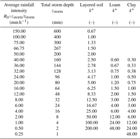
Table 2. Storm properties and dimensionless infiltration parameters

for three soils simulated.

Average rainfall Total storm depth Layered soil Loam Clay intensity zstorm k∗ k∗ k∗ R0=zstorm/tstorm

(mm h−1) (mm) (–) (–) (–)

150.00 600 0.67

100.00 400 1.00

75.00 300 1.33

66.75 267 1.50

50.00 200 2.00

40.00 160 2.50 0.60 0.30

36.00 144 2.78 0.67 0.33

32.00 128 3.13 0.75 0.38

24.00 96 4.17 1.00 0.50

20.00 80 5.00 1.20 0.75

16.00 64 6.25 1.50 1.00

12.00 48 8.33 2.00 1.50

8.00 32 12.50 3.00 2.00

6.00 24 16.67 4.00 3.00

4.00 16 25.00 6.00 4.00

2.00 8 50.00 12.00 6.00

1.00 4 100.00 24.00 12.00

0.50 2 200.00 48.00 24.00

0.25 1 48.00

The mass balance for soil water storage is accordingly given by:

dwsoil

dt =psoil(t )−qss(t )−qsat(t ) (6)

This is similar to Woods (2003) except that evaporation is ne-glected in our case. Equations 1 to 6 are solved by discretiz-ing Eq. (6) and the resultdiscretiz-ing system of algebraic equations are solved implicitly using a dynamic programming method in Mathematica 5.2 (Wolfram Research Inc., 2005).

Simulations were run for a clay, loam, sand and layered (duplex) soil for which the parameter values are listed in Ta-ble 1. Parameters for the saturated water contentθsat, field

capacityθfcand wilting pointθwpwere taken from Rawls et

al. (1992). The drainage response time,τsoil, was taken as

order of magnitude estimates from saturated hydraulic con-ductivity for a 100 mm soil depth from Rawls et al. (1992) as per Struthers et al. (2007a). The infiltration capacitiesksoil

used were 12, 24 and 100 mm h−1. This provided an order of magnitude range and a range of two orders of magnitude in the dimensionless analysis presented below. The layered soil, a coarse textured soil overlaying a finer textured soil with a sharp boundary, is commonly referred to in Australia as a duplex soil and had a high infiltration capacity and a slower drainage due to this finer textured impeding layer. This was used as these soils are common in Australia and it allowed us to test the effect of changing the ratios of infiltration ca-pacity and drainage rates. Simulations were run with initial conditions at field capacity and at wilting point.

2.2 Storm generation

Average storm properties used in the study are presented in Table 2. Total storm depth zstorm ranged from 1 to

600 mm. A constant storm duration, tstorm, of four hours

was used. The mean intensities zstorm/tstorm ranged from

0.25 to 150 mm h−1 and were chosen to allow for a wide range of scaled parameters (to be described later in Sect. 2.4) rather than to reflect the predominant rainfall intensities in Australia. The probability of these rainfall events will be discussed later in Sect. 2.5. The storm duration was kept constant for scaling purposes but initial analysis of differ-ent durations shows the same patterns of results. Four hour storms represent the approximate average storm durations in the south-west of Australia (Hipsey et al., 2003).

Rainfall intensities at these different resolutions were gen-erated using the bounded random cascade model (Menabde and Sivapalan, 2000) firstly parameterized to south-western Australian rainfall (Hipsey et al., 2003). Random cascades are based on the apparent multifractal scaling behaviour of rainfall. Rainfall variability at different time scales is de-termined by the analysis of break down coefficients,u(τ, i), which are defined as “the ratio of rainfall of a random field averaged over different scales where the smaller is contained within the larger” (Harris et al., 1998, pp. 93):

u(τ, i)=Rτ(tn) Ri(tn)

τ < i (7)

whereRτ (tn) andRi (tn) are the rainfall totals accumulated

over the durationsτ andi whereτ is assumed to be com-pletely included in the intervali (Menabde and Sivapalan, 2000). For a more detailed description of breakdown coef-ficients and their analysis see Harris et al. (1998). Menabde and Sivapalan (2000) explain how the breakdown coefficients for the entire rain record is separated into different time inter-vals and the distributions of breakdown coefficients at differ-ent timescales is described by fitting a single parameter beta distribution:

pU(u)=

1

B(a)u

a−1_(1−u)a−1_,

whereB(a)= Z 1

0

xa−1(1−x)a−1dx (8)

with the sole parameterachanging with the timescale of ob-servation t. It has been found in a number of studies that at smaller timescales the breakdown coefficients are more similar (less variable) and breakdown coefficients at larger timescales are more variable (Menabde et al., 1997; Harris et al., 1998; Menabde and Sivapalan, 2000). Menabde and Sivapalan (2000) use the following scaling law to describe this dependence of theaparameter on the timescale,t:

a(t )=a0t−H (9)

A high or largea0parameter (yintercept) means that rainfall

at small timescales is less variable (more constant). In

con-trast, a low or smalla0parameter would indicate more

vari-ability of rainfall intensities at small time intervals. TheH

parameter describes the slope of this relationship and hence the rate of change of variability with increasing time inter-vals.

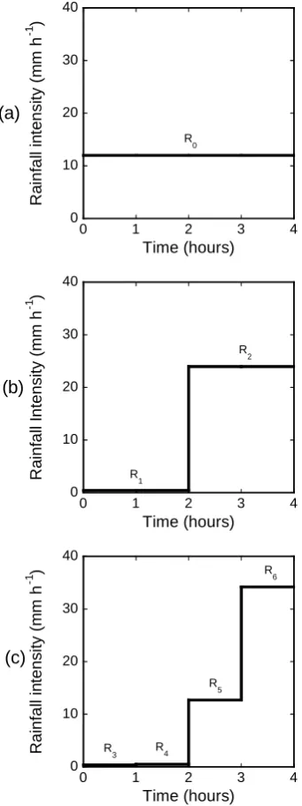
Rainfall is generated by starting with an initial homoge-neous storm of a certain length (tstorm)and average storm

intensityR0. The next step is to divide the original storm

du-ration (tstorm)into two halves and assign each half a valueR1

andR2where the sum ofR1t andR2t=R0tand the weights

at any leveln, are drawn from the beta distribution with its sole parameteraestimated from relationship (9). See Fig. 2 for an example of storm intensities generated for three dif-ferent time scales (t). For further details on the generation of rainfall see Menabde and Sivapalan (2000).

The four hour storm duration was long enough to investi-gate 6 cascades of rainfall resolutions (120, 60, 30, 15, 7.5, 3.75, 1.875 min) with the resolution halving at each cascade (tn=2nt0) with n=0, 1 ,2, . . . 6 andt0=1.875 min. To ensure

that rainfall input into the rainfall partitioning model was at the same resolution (1.875 min), all input vectors had a length of 128 (240/1.875). Intensities at lower resolutions were repeated (time step (tn)/1.875) times so that all vector lengths were the same.

An initial analysis of distributions of storms generated us-ing the model was conducted to determine a statistically sta-ble number of storm realizations to be used in the analysis. The first, second and third moments were calculated for dis-tributions of rainfall intensities from x realizations of a storm event (x= 25, 50, 100, 250, 500, 750, 1000, 2000). Atx=500 the variations in the moments converged so that distributions withxvalues greater than 500 were not significantly different (T test, p=0.05) fromx=500. For this reason, five hundred realizations of each storm were used in the analysis. 2.3 Output analysis

At the end of each simulation the total amount of infiltration excess, saturation excess, deep drainage and runoff were cal-culated (mm). The first, second and third moments of the distributions of these amounts as well as the distributions of the maximum intensities (mm min−1_{), frequencies and}

dura-tions (min) each surface runoff process was active through-out each storm event. The moments of the distributions of the scaled outputs were also calculated and used to compare the response of different soils to different storm properties. 2.4 Scaling of outputs

0 10 20 30 40

0 1 2 3 4

R

a

in

fa

ll in

te

n

s

it

y

(

m

m

h

-1 )

Time (hours) R

0

0 10 20 30 40

0 1 2 3 4

Rainfa

ll I

n

tensity (mm h

-1 )

Time (hours) R

1

R 2

0 10 20 30 40

0 1 2 3 4

R

a

in

fa

ll in

tensity (m

m

h

-1 )

Time (hours) R

3 R4

R 5

R 6 (a)

(b)

(c)

Figure 2. Diagram of rainfall generation at cascading time steps (4 hours, 2 hours and 1

hour).

35

Fig. 2. Diagram of rainfall generation at cascading time steps (4 h,

2 h and 1 h).

depth making them dimensionless. These dimensionless out-puts were related to three dimensionless scaling parameters that were derived from three groups of dimensional parame-ters that characterise the soil and the averaged rainfall prop-erties. The soil parameters were the infiltration capacityksoil

(Eq. 1) and the ratio of soil depth and drainage response time zsoil/τsoil (Eq. 3) controlling the drainage behaviour.

From here on this ratio (zsoil/τsoil)will be referred to as the

drainage coefficient. The average rainfall was fully charac-terized by the average intensityzstorm/tstorm. All groups were

rates in mm min−1and ratios of these groups were used to carry out the scaling analysis presented below.

Infiltration excess was produced when the supply of water (rainfall) exceeded the soil infiltration capacity threshold. By relating these two properties we could determine the amount of dimensionless infiltration excess for a range of infiltration capacities and average storm intensities using one curve. The scaling parameter we used to do this wask∗ (–) which is the ratio of maximum soil infiltration capacity to the average storm intensity:

k∗= ksoiltstorm zstorm

(10) The range ofk∗values was 0.3 to 200 (Table 2). The higher the average storm intensity relative to the infiltration capacity is, the smaller thek∗value.

Saturation excess occurred when the difference between the flux of water entering the soil and the flux of water leaving the soil (drainage) exceeded the soil storage capac-ity. The second dimensionless parameter,f∗(–), relates soil properties controlling the input of water (infiltration capacity,

ksoil)to the drainage coefficient (zsoil/τsoil)which represents

the soil properties controlling the output of water:

f∗= ksoilτsoil zsoil

(11) The higher the infiltration rate multiplied by the drainage rate the deeper the soil required to maintain the samef∗ value. The range off∗ values is presented in Table 1. The range of f∗ parameters was limited to soil depths no shallower than 100 mm. For the sand, with a high infiltration capac-ity and fast drainage rate even at the shallowest soil depth (100 mm) no saturation excess was produced, making this the only depth simulated.

Now the soil properties that control saturation excess have been scaled (usingf∗) we need to relate them to the storm properties that produce saturation excess. By doing this we could determine the storm properties at which saturation ex-cess was most sensitive to rainfall resolution for our range off∗parameters. This was done by constructing theg∗ pa-rameter which is the average storm intensity in relation to the drainage coefficient:

g∗= tstormzsoil zstormτsoil

= k

∗

f∗ (12)

2.5 Application to different rainfall regions

To investigate the influence of rainfall generated from dif-ferent rainfall regions we concentrated on infiltration excess predictions as we have already discussed the limitations of applying the saturation excess predictions. We began by looking at how the within storm temporal variability influ-ences the soil-storm scaling relationship outlined above. We then looked at the average storm intensities of different lo-cations and the fraction of storms for each location likely to affect infiltration excess predictions if low resolution rainfall is used.

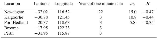
Table 3. Rainfall data and bounded random cascade parameters for locations in different rainfall regions in Western Australia.

Location Latitude Longitude Years of one minute data a0 H

Newdegate −32.02 116.52 22 15.0 −0.47

Kalgoorlie −30.78 121.45 3 10.8 −0.44

Port Hedland −20.37 118.63 3 5.8 −0.35

Broome −17.95 122.23 3

Perth −31.95 115.87 3

To investigate the effect of different within storm patterns from different rainfall regions rainfall was generated using

a0 andH parameters fitted to rainfall from three locations

in Western Australia. These locations included Newdegate, Kalgoorlie and Port Hedland. The parameterization of the bounded random cascade model to 15 different locations in Western Australia found that Newdegate had the least within storm variability, Port Hedland had the most variable within storm patterns and Kalgoorlie was in between (Hearman and Hinz, 20071). See Table 3 for these parameters. Newde-gate is located in the south west, the same location as Hipsey et al. (2003) and experiences predominantly winter rainfall (June to August) in the form of advective fronts. Port Hed-land and Kalgoorlie are located in arid regions of the state. Port Hedland is in the tropics and receives convective and cy-clonic rain predominantly in the summer months. Kalgoorlie is located further south and inland and has less intense and less seasonal rainfall. The same point scale rainfall partition-ing model and soil-storm scalpartition-ing (as outlined above) was ap-plied to rainfall generated from these three locations and the effect of different within storm variability on the differences in point scale infiltration excess predictions using different rainfall resolutions was determined.

An investigation of the effect of locations in different rain-fall regions on the likelihood infiltration excess predictions will be affected by rainfall resolution was done using one minute rainfall data from five locations in Western Australia. These locations included the three outlined above, as well as Broome, located in the north east of Western Australia and experiencing summer monsoonal rain, and Perth, located on the coast of the south west region. This was done by calcu-lating average storm intensities from the one minute rainfall where a storm was identified as having 7 h between rainfall measurements. Then, using the average storm intensities,k∗

values were calculated for clay, loam and sandy soils. From the results of the scaling of differences in infiltration excess predictions using different rainfall resolutions we were able to identify the fraction of storms where rainfall resolution was likely to affect infiltration excess predictions using the calculatedk∗values for each soil from each location.

1_{Hearman, A. J. and Hinz, C.: Within storm rainfall variability}

in Western Australia, in preparation, 2007.

3 Results and discussion

3.1 Model output

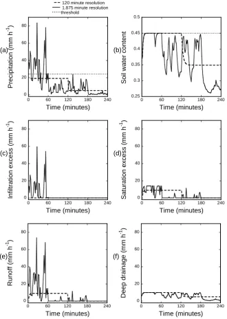
The rainfall resolution influenced the amount and dynamics of infiltration excess and saturation excess runoff predictions. Figure 3 is an example of the model output for a single storm event showing two different rainfall resolutions; 1.875 min (black line) and 120 min (broken line). From this figure it can be seen that the higher resolution rainfall had higher peaks in intensities than the low resolution rainfall. This lead to infil-tration excess being triggered when high resolution rainfall was used and not when the low resolution rainfall was used. As a result more water was able to enter the soil for the low resolution rainfall and the soil was saturated for a longer pe-riod of time.

Figure 3 demonstrates that not only were the processes that generated runoff different for the two different rainfall reso-lutions but also the dynamics of runoff produced from the dif-ferent rainfall resolutions. High resolution rainfall generated more runoff with higher peaks in intensity. From this exam-ple we illustrate that rainfall resolution has a direct impact on the triggering of thresholds, in particular, infiltration excess. Models using time averaged rainfall would need to calibrate this threshold to a lower effectiveksoilif they are to fit their

model predictions to field measurements. However, even if the model is able to be calibrated to give the correct infil-tration excess amount, using low resolution rainfall will give different dynamics. Low resolution rainfall will lead to long, low intensity predictions of runoff, whereas high resolution rainfall will lead to short, more intense bursts of runoff. The implications of these different surface runoff dynamics will be discussed later in the dynamics Sect. 3.5.

Whilst Fig. 3 is an example of one storm realization, the results presented in the sections that follow consider the sta-tistical properties of the response, in particular the means of the distributions produced from 500 of these realizations and how these relate to scaled soil-storm properties.

3.2 Infiltration excess

0 20 40 60 80

0 60 120 180 240

120 minute resolution 1.875 minute resolution threshold

P

rec

ip

it

at

io

n

(

m

m

h

-1 )

Time (minutes)

(a)

0.25 0.3 0.35 0.4 0.45 0.5

0 60 120 180 240

So

il w

ate

r conte

n

t

Time (minutes)

(b)

0 20 40 60 80

0 60 120 180 240

In

fi

ltr

a

ti

on

ex

c

e

s

s

(

m

m h

-1 )

Time (minutes)

(c)

0 20 40 60 80

0 60 120 180 240

Sa

tu

ra

ti

o

n

e

x

c

e

s

s

(

m

m

h

-1 )

Time (minutes)

(d)

0 20 40 60 80

0 60 120 180 240

Ru

no

ff

(mm h

-1 )

Time (minutes)

(e)

0 20 40 60 80

0 60 120 180 240

D

e

e

p

d

rain

age

(

m

m h

-1 )

Time (minutes)

(f)

Figure 3. Example of the model input (precipitation (a)) and model outputs (soil water

content (b), infiltration excess (c), saturation excess (d), runoff (e) and deep drainage (f)).

Produced from one storm (48 mm) at two different rainfall resolutions (1.875 min and

120 min) for a loam soil with a depth of 100 mm.

36

Fig. 3. Example of the model input (precipitation (a)) and model outputs (soil water content (b), infiltration excess (c), saturation excess (d),

runoff (e) and deep drainage (f)). Produced from one storm (48 mm) at two different rainfall resolutions (1.875 min and 120 min) for a loam soil with a depth of 100 mm.

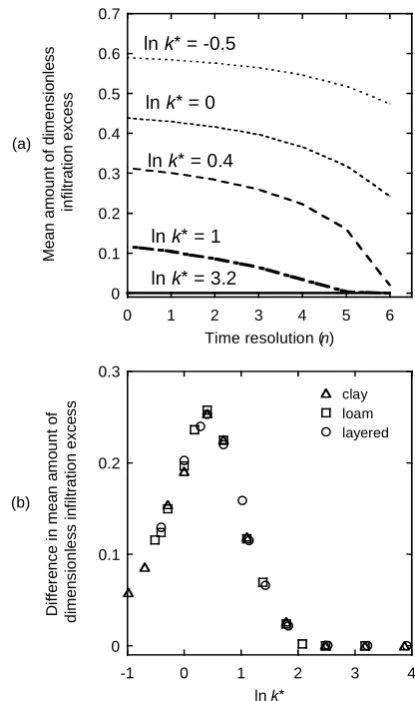
(n=0) produced more infiltration excess than the low resolu-tion rainfall of 120 min (n=6). This figure also demonstrates that for differentk∗values, the slopes of these curves, or the sensitivity to rainfall resolution were different. The sensitiv-ity of predicted amounts of infiltration excess was summa-rized in Fig. 4b which shows the differences in infiltration amounts between 1.875 min resolution and 120 min resolu-tion, which is the first point minus the last point for each curve in Fig. 4a. It can be seen that the scaling allows the

curves for all soil types to collapse. They were most sensi-tive to rainfall resolution when the soil infiltration rate was 1.5 times the average storm intensity (lnk∗=0.4), and at this point the amount of infiltration excess was under predicted by 26% of the total storm amount. This supports Bronstert and Bardossy (2003) who also found that the sensitivity of predictions of infiltration excess to rainfall resolution were highest where the average rainfall intensity was in the same order of magnitude as the infiltration capacity of the soil.

Analysis of differences between smaller time steps (than our maximum 120 min) and our smallest time step (1.875 min) show that the biggest differences also occur at lnk∗=0.4. Using 15 min resolution (n=3) still under pre-dicted infiltration excess by 20% and 3.75 min resolution (n=1) under predicted infiltration excess by 10% of the to-tal storm volume at lnk∗=0.4. This implies that at the point scale when the soil infiltration rate is near 1.5 times the aver-age storm intensity the rainfall resolution will impact runoff predictions even at resolutions less than 5 min. These re-sults contradict Bronstert and Bardossy (2003) who found that between 5 min and 1 min there was no significant dif-ference in surface runoff predictions. This may be the result of runoff transformation processes down the hillslope as our analysis is conducted at the point scale and Bronstert and Bardossy’s (2003) at the hillslope scale or a result of having an infiltration rate that changes with time. When an initial infiltration amountF0was introduced before the soil

infiltra-tion capacity started taking effect, the maximum difference for infiltration excess predictions using different rainfall res-olutions remained at lnk∗=0.4 but the size of the differences decreased with increasingF0. Also for surface runoff

predic-tions at larger scales not only is the interaction of infiltration properties and storms important but also hillslope properties that control runoff response times (Woolhiser and Goodrich, 1988).

The sensitivity of point scale infiltration excess predic-tions to rainfall resolupredic-tions can be explained by the way the different rainfall resolutions triggered the infiltration excess threshold. At lnk∗values greater than 1.5, neither the high resolution rainfall nor the low resolution rainfall intensities were high enough to trigger infiltration excess. Where lnk∗

was between 1.5 and 0.4, increasing the intensity of the storm lead to an increase in the amount of infiltration excess trig-gered by the high resolution rainfall, whereas the low resolu-tion rainfall intensities were not high enough to trigger this threshold. Where lnk∗ was less than 0.4, the dimensionless difference in infiltration excess amounts decreased. This was because at lnk∗=0.4, infiltration excess was first triggered in the low resolution rainfall. The amount of infiltration excess then increased more rapidly for the low resolution rainfall than for the high resolution rainfall. This was because the low resolution rainfall had longer time steps so once these intensities began to trigger the threshold they spent a longer period of time above the threshold. At lnk∗=0.4, where the maximum difference between the two resolutions occurred, the low resolution rainfall first triggered the infiltration ex-cess threshold and therefore became the point where the biggest difference between the amounts of infiltration excess produced from the different rainfall resolutions occurred (see Fig. 7e(i), 7f(i)).

These results highlight how point scale infiltration excess predictions can be influenced by rainfall resolution and the sensitivity of these predictions to rainfall resolution depends on the relationship between rainfall intensities and soil

infil-0 0.1 0.2 0.3 0.4 0.5 0.6 0.7

0 1 2 3 4 5 6

M

ean

am

o

un

t

o

f

di

m

e

nsi

o

nl

e

s

s

i

n

fi

lt

ra

ti

on exce

s

s

Time resolution (n) ln k* = -0.5

ln k* = 0

ln k* = 0.4

ln k* = 1

ln k* = 3.2

(a)

0 0.1 0.2 0.3

-1 0 1 2 3 4

loam clay

layered

D

if

fe

ren

c

e

i

n

m

e

an

a

m

o

u

n

t of

di

m

e

n

s

ionl

e

s

s in

fi

lt

ra

ti

on

exc

e

ss

ln k*

(b)

Figure 4. The changes in mean amount of dimensionless infiltration excess with the 7

different time resolutions tested (n= 0,1,2….6, t

=2

t

where t

= 1.875 min) for a loam

soil at various mean rainfall intensities relative to the infiltration capacity,

k

* (a) and the

difference in mean dimensionless amount of infiltration excess between 1.875 and 120

min resolution according to changes in the natural log of

k

* for the clay, loam and

layered soils (b).

37

Fig. 4. The changes in mean amount of dimensionless

infiltra-tion excess with the 7 different time resoluinfiltra-tions tested (n=0,1,2. . . 6,

tn=2nt0wheret0=1.875 min) for a loam soil at various mean

rain-fall intensities relative to the infiltration capacity, k∗ (a) and the

difference in mean dimensionless amount of infiltration excess be-tween 1.875 and 120 min resolution according to changes in the nat-ural log ofk∗for the clay, loam and layered soils (b).

0 0.1 0.2 0.3 0.4

0 1 2 3 4 5 6

Mean a

mount o

f d

im

e

n

s

io

n

le

s

s

sat

u

ra

ti

o

n

e

xces

s

Time resolution (n) ln k* = -0.5

ln k* = 0.2

ln k* = 1

ln k* = 3.2 f* = 0.48

Figure 5. The changes in mean amount of dimensionless saturation excess with the

natural log of the 6 different time resolutions tested (n=0,1,2…6, t

=2

t

where t

=

1.875 min for a loam soil with an initial water content at field capacity for storms with

different mean rainfall intensities relative to the infiltration capacity (

k

*).

38

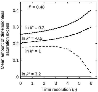
excess with the natural log of the 6 different time resolutions tested (n=0,1,2. . . 6,tn=2nt0wheret0=1.875 min for a loam soil with an

initial water content at field capacity for storms with different mean rainfall intensities relative to the infiltration capacity (k∗).

al., 2005) this simple method could prove useful in gaining an understanding of whether high resolution rainfall data is required to accurately predict surface runoff for a particular location.

3.3 Saturation excess

Whilst the saturation excess predictions cannot be applied in such a direct way as the infiltration excess sensitivity curve due to larger scale processes which are not considered here, the authors believe the saturation excess results illustrate how rainfall resolution can influence a surface runoff generating mechanism that is buffered by soil water storage and depen-dent on the differences in soil infiltration created from the interaction of the different rainfall resolutions and the infil-tration capacity threshold.

Many surface runoff models do not attempt to model both surface runoff generating mechanisms (infiltration excess and saturation excess) and instead assume one or the other. Whilst previous studies of Australian surface runoff indicate that infiltration excess or Hortonian overland flow is the pre-dominant mechanism, in other climates and regions of the world (more humid) surface runoff can be dominated by sat-uration excess or change between satsat-uration excess and infil-tration excess seasonally. Our results indicate that under cer-tain soil-storm properties rainfall resolution may influence what process may dominate predicted surface runoff genera-tion.

Our simulations indicated that for soils with a drainage coefficient greater than 5 times the infiltration capacity,

f∗≤0.2, no saturation excess was triggered by either

rain-fall resolution. These findings enabled us to split our soil into two groups, those susceptible to saturation excess with

f∗ values greater than 0.2 (which will be presented in this section) and those not susceptible to saturation excess with

f∗values equal or less than 0.2. That is, fast draining and/or deep soils were not likely to produce saturation excess un-less influenced by a rising water table or topographic features (not considered here). This means for the fast draining sand tested, withf∗=0.2, even at a shallow soil depth of 100 mm no saturation excess was produced from either rainfall res-olution (assuming the lower boundary is highly permeable). The effect of having a less permeable lower boundary was investigated by using a layered soil with a high infiltration capacity (the same as the sand) but a slower drainage re-sponse time. Unless stipulated, the following results show simulations where the initial soil water content was at field capacity.

Using low resolution rainfall in soils with f∗ values greater than 0.2 resulted in either an over prediction or an under prediction of saturation excess depending on the soil-storm relationships. Figure 5 shows how the amount of pre-dicted saturation excess changed with different rainfall reso-lutions (x-axis) and with different storm intensities (various

k∗values). The figure illustrates that for high rainfall intensi-ties (lowk∗values) a low resolution rainfall predicted more saturation excess than at high resolutions. As we decreased the average intensity of the storm (increase thek∗value) this difference became smaller to a point where the high resolu-tion rainfall predicted more saturaresolu-tion excess than the low resolution rainfall.

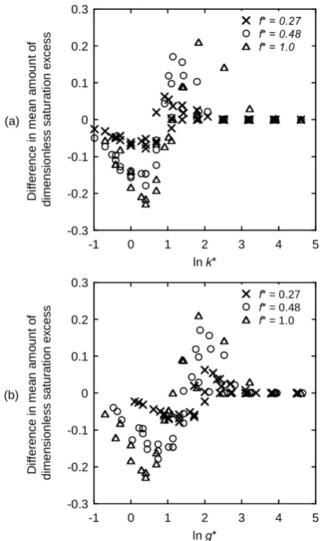
These differences in predictions of saturation excess using 1.875 min rainfall and 120 min rainfall (i.e. the mean amount predicted using 1.875 min rainfall minus the mean amount predicted using 120 min rainfall) for different soil types and soil depths are shown in Fig. 6. From this graph it can be seen that the maximum difference in over predictions of saturation excess (where the differences are most negative) scale with

k∗ and occur at lnk∗=0.4. This is because this is the point where there is the biggest difference in predictions of infil-tration excess and therefore the biggest difference in amount of water entering the soil. The low resolution rainfall had no infiltration excess at this point so more water was able to en-ter the soil and this combined with the constant rainfall inten-sity lead to a greater prediction of saturation excess than that predicted using the high resolution rainfall. This highlights the interaction of the two different thresholds (infiltration ca-pacity and soil storage caca-pacity) and how the input resolution can control which process dominates surface runoff.

These results also highlight the differences in water able to enter the soil depending on the rainfall resolution. Our re-sults show that for high average intensity storms using low resolution rainfall over predicts the amount of water enter-ing the soil and may result in an over prediction of processes affected by soil water storage such as drainage and subsur-face flow predictions, the leaching of agri-chemicals and our

understanding of the ecology of plant species and their adap-tation to certain soil-water conditions.

The size of the over prediction of saturation excess with low rainfall resolution depended on the ratio of infiltration capacity to drainage coefficient, f∗, with higher f∗ val-ues (shallower soils relative to the infiltration capacity and drainage coefficient) resulting in bigger differences in pre-dictions (more negative) of saturation excess. This was be-cause less water was required to saturate the soil profile so more saturation excess was predicted from the same amount of water entering the soil profile and thus resulted in bigger differences in predictions from different rainfall resolutions. From Fig. 6a it can be seen that the maxima of the pos-itive differences did not all occur at the same lnk∗ value. This was because infiltration excess was not being triggered at such low intensity storms. Instead, the maximum differ-ences depended on how fast the soil was draining in relation to how fast the water was entering the soil i.e. theg∗ param-eter. Figure 6b presents the differences in amounts of satura-tion excess according to changingg∗values. It can be seen that the maxima of the positive differences in saturation ex-cess occur when the saturated drainage rate was 7.4 times the average storm intensity (lng∗=2). This was the point where low resolution rainfall began to trigger the storage capacity threshold. These results show that in soils susceptible to sat-uration excess, surface runoff predictions can be affected by rainfall resolutions at lower intensity storms than soils not susceptible to saturation excess. It also demonstrates that at lower average intensity storms the rate at which water enters the soil may be under predicted with the use of low reso-lution rainfall and therefore result in an under prediction of drainage and the potential for the leaching of agri-chemicals. In Fig. 6 it can be seen that the size of the negative dif-ferences clearly relate to thef∗values, but the positive dif-ferences are more variable. This can be explained by the scaling methods used. The scaling related steady state con-ditions or the average storm intensity to soil properties, but it did not account for the variations in intensities throughout a storm when smaller time steps were used (higher resolu-tion rainfall). The soil storage capacity was scaled relative to steady state infiltration and drainage rates and did not ac-count for the variations in the rate of water entering the soil when high rainfall resolutions were used. When the rain-fall intensity exceeded the infiltration capacity the water en-tered the soil at a constant intensity (equal to the infiltration capacity) and this is why the negative differences in satu-ration excess scale with thef∗parameter. However, when the rainfall intensity did not exceed the soil infiltration ca-pacity and the input was high resolution rainfall the water entered the soil at variable intensities. But the scaling did not account for the range in the rates that water could enter the soil. For this reason, differences in amounts of satura-tion excess between high resolusatura-tion rainfall and steady state conditions were different for the soil types simulated even though these soils have the samef∗andg∗scaling

parame--0.3 -0.2 -0.1 0 0.1 0.2 0.3

-1 0 1 2 3 4 5

f* = 0.27 f* = 0.48 f* = 1.0

D

if

fe

ren

c

e

i

n m

e

an

am

o

u

n

t of

d

imens

ionl

e

s

s s

a

tu

ra

ti

o

n

e

x

ces

s

ln k* (a)

-0.3 -0.2 -0.1 0 0.1 0.2 0.3

-1 0 1 2 3 4 5

f* = 0.27 f* = 0.48 f* = 1.0

D

if

fe

ren

c

e

i

n m

e

an

am

ou

n

t of

dime

ns

ion

le

s

s

sa

tu

ra

ti

on

ex

c

e

ss

ln g* (b)

Figure 6. The difference in mean dimensionless amount of saturation excess between

1.875 and 120 min resolution according to changes in a) the natural log of

k

* and b) the

natural log of

g*

for the clay, loam and layered soils with

f*

values of 0.27, 0.48 and 1

and initial soil water contents at field capacity.

Fig. 6. The difference in mean dimensionless amount of saturation

excess between 1.875 and 120 min resolution according to changes in (a) the natural log ofk∗and (b) the natural log ofg∗for the clay, loam and layered soils withf∗values of 0.27, 0.48 and 1 and initial soil water contents at field capacity.

ters. For example, the clay soil, with a much slower drainage response time (τsoil)required a deeper soil (5 times) to have

the same drainage coefficient in relation to maximum infiltra-tion rate than the loam soil. But the range of intensities enter-ing the clay soil was only 0–12 mm h−1in comparison to 0– 24 mm h−1of the loam. Meaning that the clay soil requires a higher average intensity storm relative to the drainage coeffi-cient (smallerg∗value) before the storage capacity threshold is exceeded.

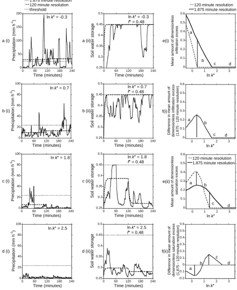
An illustration of how using low resolution rainfall can change from an over prediction of saturation excess to an under prediction of saturation excess is shown in Fig. 7. This figure illustrates examples of different storms and dif-ferent “stages” of threshold triggering and how this threshold

0 50 100 150 200

0 60 120 180 240

1.875 minute resolution 120 minute resolution threshold P rec ip it a tio n ( m m h -1 ) Time (minutes) a (i)

ln k* = -0.3

0.25 0.3 0.35 0.4 0.45 0.5

0 60 120 180 240

Soi l wa te r sto rag e Time (minutes) a (ii)

ln k* = -0.3

f* = 0.48

0 0.1 0.2 0.3 0.4 0.5 0.6

0 1 2 3

120 minute resolution 1.875 minute resolution

M e an a m o unt o f d im e n s io n les s in fi lt ra ti o n e x ce ss

ln k*

e(i) d c b a 0 20 40 60 80 100

0 60 120 180 240

P re c ip it a tio n ( m m h -1 ) Time (minutes) b (i)

ln k* = 0.7

0.25 0.3 0.35 0.4 0.45 0.5

0 60 120 180 240

S o il w a te r st or ag e Time (minutes) b (ii)

ln k* = 0.7

f* = 0.48

0 0.1 0.2 0.3 0.4 0.5 0.6

0 1 2 3

D if fe re n c e in m e an am o u n t o f di m e ns io n le s s i n fil tr a ti o n e x ce s s (1. 8 75 120 m in u te r e s ol ut ion )

ln k* f(i) a b c d 0 20 40 60 80 100

0 60 120 180 240

P recip ita tio n ( m m h -1 ) Time (minutes) c (i)

ln k* = 1.8

0.25 0.3 0.35 0.4 0.45 0.5

0 60 120 180 240

Soi l wa te r s to rag e Time (minutes) c (ii)

ln k* = 1.8

f* = 0.48

0 0.1 0.2 0.3 0.4 0.5 0.6

0 1 2 3

120 minute resolution 1.875 minute resolution

M e a n a m o u nt o f d im e ns io nl es s s a tu rati o n ex c e s s

ln k*

e(ii) _a b c _d 0 20 40 60 80 100

0 60 120 180 240

P re c ip it at io n ( m m h -1 ) Time (minutes) d (i)

ln k* = 2.5

0.25 0.3 0.35 0.4 0.45 0.5

0 60 120 180 240

So il wa te r stora g e Time (minutes) d (ii)

ln k* = 2.5

f* = 0.48

-0.2 -0.1 0 0.1 0.2 0.3 0.4 0.5 0.6

0 1 2 3

Di ff er en c e i n m e a n a m o u n t o f di m e n s io nl es s s a tu ra ti on e x c es s (1 .8 7 5 1 2 0 mi nu te r e s o lu ti on )

ln k*

f(ii)

a b

c d

Figure 7. An illustration of the different ‘stages’ of threshold triggering; both resolutions

trigger the thresholds (a(i) & a(ii)), only the high resolution triggers the infiltration excess

threshold (b(i)) and both resolutions trigger the storage threshold (b(ii)), only the high

resolution rainfall triggers the saturation excess threshold (c(ii)) and neither resolution

triggers either of the thresholds (d(i) & d(ii)) and how these different ‘stages’ relate to

total storm infiltration excess (e(i)) and saturation excess (e(ii)) for two different

resolutions and the differences in these predictions (f(i) &f(ii)) for the two resolutions.

40

Fig. 7. An illustration of the different “stages” of threshold triggering; both resolutions trigger the thresholds (a(i) and a(ii)), only the high

resolution triggers the infiltration excess threshold (b(i)) and both resolutions trigger the storage threshold (b(ii)), only the high resolution rainfall triggers the saturation excess threshold (c(ii)) and neither resolution triggers either of the thresholds (d(i) and d(ii)) and how these different “stages” relate to total storm infiltration excess (e(i)) and saturation excess (e(ii)) for two different resolutions and the differences in these predictions (f(i) and f(ii)) for the two resolutions.

A. J. Hearman and C. Hinz: Sensitivity of point scale runoff predictions to rainfall 977 triggering also interacts with changes in the triggering of

in-filtration excess.

While the initial soil moisture made a difference to the amount of surface runoff predicted it only made a small dif-ference to the difdif-ferences in predicted amounts of saturation excess between high and low resolution rainfall.

3.4 Surface runoff

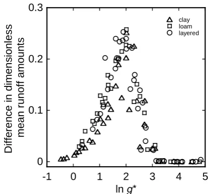
Total surface runoff was a combination of infiltration excess and saturation excess and was always under predicted by low resolution rainfall (Fig. 8). The biggest differences in surface runoff occurred on soils where maximum infiltration capaci-ties were equal to or less than 1/5th of the drainage coefficient (f∗≤0.2), when no saturation excess was produced so all surface runoff was attributed to infiltration excess. Whenf∗

was greater than 0.2, saturation excess started to be produced and surface runoff became more sensitive to rainfall resolu-tions at lower intensity storms. Surface runoff predicresolu-tions were most sensitive to rainfall resolution when the drainage coefficient was 7.4 times greater than average rainfall inten-sity (lng∗=2). The biggest differences in total surface runoff were the same as the biggest positive differences in satura-tion excess. This was because at this point low resolusatura-tion rainfall was not producing any surface runoff and high res-olution rainfall was producing saturation excess runoff. At higher rainfall intensities (lowerg∗), the difference in total surface runoff amounts was smaller, but this was because the low resolution rainfall was predicting saturation excess runoff, in contrast to the high resolution rainfall which was predicting more infiltration excess. So although the sensi-tivity of total amounts of surface runoff appears to be lower at high intensity storms (lowerg∗), the process that domi-nated runoff depended on the rainfall resolution. This will not only affect the dynamics of predicted surface runoff but also predicted amounts of water entering the soil and there-fore predictions of soil moisture and drainage (as discussed in the saturation excess section). This is strictly valid where two and three dimensional processes such as lateral subsur-face flow and groundwater interaction are negligible. This may be the case on the upper parts of a hillslope where there is no lateral flow of water.

Figure 8 has been presented according to soil types. At

f∗_{=0.2, where all surface runoff was attributed to infiltration}

excess, the differences in predictions for all soil types were the same. Forf∗ values greater than 0.2 the slower ing clay soil had smaller differences than the faster drain-ing loam and layered soils for reasons outlined in the satura-tion excess secsatura-tion. Thus, predicsatura-tions of surface runoff, for all soils, were most sensitive to rainfall resolutions when all runoff was attributed to infiltration excess only.

0 0.1 0.2 0.3

-1 0 1 2 3 4 5

clay loam layered

Dif

fer

e

n

ce in

dimen

s

ionl

es

s

me

an

ru

no

ff

a

m

o

u

n

ts

ln g*

Figure 8. The difference in dimensionless surface runoff between 1.875 and 120 min

resolution according to the natural log of

g*

for

f*

values of 0.20, 0.27 and 0.48 for clay,

loam and layered soils.

41

Fig. 8. The difference in dimensionless surface runoff between

1.875 and 120 min resolution according to the natural log ofg∗for

f∗values of 0.20, 0.27 and 0.48 for clay, loam and layered soils.

3.5 Dynamics

0 0.5 1 1.5 2 2.5 3

-1 0 1 2 3 4

loam clay layered D if ferenc e in di m e ns ionless m e an ma x im u m infi lt ra ti o n e x c e s s

ln k*

a(i) 0 0.5 1 1.5 2 2.5 3

-1 0 1 2 3 4

layered loam clay Di ff ere n c e i n di m ens io n les s m ean m ax im um s at u rat ion exc es s

ln k*

a(ii) 0 2 4 6 8 10 12

-1 0 1 2 3 4

loam clay layered Dif fer e n c e i n f requ e nc y inf ilt ra ti o n exces s i s t ri ggere d

ln k*

b(i) 0 2 4 6 8 10 12

-1 0 1 2 3 4 5

layered loam clay D if fe re n c e in freq uency s a tu ra ti o n e x c e ss is tri g g e re d

ln g*

b(ii) -100 -80 -60 -40 -20 0

-1 0 1 2 3 4

loam clay layered D if fe re n c e i n ti m e i n fi ltr a ti o n exc e ss i s ac ti ve ( m in )

ln k*

c(i) -100 -80 -60 -40 -20 0

-1 0 1 2 3 4 5

layered loam clay Di ff erenc e in tim e s a tu ra tion ex c e ss is ac ti ve ( m in )

ln g*

c(ii)

Figure 9. Differences in the dynamics of infiltration excess (i) and saturation excess (ii)

for clay, loam and layered soils with changing soil-storm properties (ln

k

* and ln

g

*).

These dynamics include dimensionless mean maximum intensities (a), frequencies the

threshold was triggered (b) and time the process was active during the storm (c).

42

Fig. 9. Differences in the dynamics of infiltration excess (i) and saturation excess (ii) for clay, loam and layered soils with changing soil-storm

properties (lnk∗and lng∗). These dynamics include dimensionless mean maximum intensities (a), frequencies the threshold was triggered

(b) and time the process was active during the storm (c).

3.6 Implications for larger scale predictions

The implication of these findings to larger scales, such as the hillslope, is uncertain. Whilst our point scale results support the hillslope results of Bronstert and Bardossy (2003) who also found that the sensitivity of predictions of infiltration excess to rainfall resolution were highest when the average rainfall intensity was in the same order of magnitude as the

infiltration capacity, previous studies on the effects of rainfall resolution on hillslope runoff predictions have had mixed re-sults. Numerous larger scale (hillslope to catchment) studies have concluded that temporally averaging rainfall inputs re-sulted in under predictions of runoff amounts and peak runoff intensities (Bronstert and Bardossy, 2003; Wainwright and Parsons, 2002; Singh, 1997; Woolhiser and Goodrich, 1988). In constrast, Reaney et al. (2007) showed that the temporal

averaging of rainfall inputs can result in either an over pre-diction or an under prepre-diction of hillslope surface runoff. Ex-perimental studies have shown the importance of temporal rainfall structure on hillslope runoff lengths (Stomph et al., 2002; Puigdefrabregas, 1999). Puigdefabregas (1999) ex-plains that pauses in rainfall allow overland flows to infiltrate and thus constrains overland flow lengths. In contrast, long lasting saturation excess overland flow covers greater dis-tances (Puigdefabregas, 1999). Cameraat (2004) illustrated that the frequency of rainfall events that trigger plot scale runoff was higher than the frequency of rainfall events that trigger hillslope or catchment runoff, illustrating that at the finest scales, soil properties such as infiltration capacity are very important in controlling runoff triggering, whereas at larger scales, such as the plot and hillslope, the spatial pat-tern of vegetation plays an important role in the triggering of runoff thresholds. These experimental studies highlight the complex nature of scaling point scale runoff predictions to larger scale runoff predictions which is beyond the scope of this paper.

3.7 Application to other rainfall regions

When the same sensitivity analysis was applied using differ-ent rainfall parameters (more variable rainfall from the trop-ics) the maximum differences between runoff predicted from high and low resolution rainfall occurred at the same soil-storm properties. That is, maximum differences in infiltra-tion excess occurred at lnk∗=0.4. However with more vari-able rainfall these maximum differences were larger. Port Hedland, with the most variable rainfall analysed, had dif-ferences in infiltration excess predictions between 1.875 min and 120 min rainfall resolutions of 34% as compared to 26% using south west rainfall parameters (Newdegate). This illus-trates that for all rainfall types this peak sensitivity of point scale surface runoff predictions to rainfall resolutions occurs at the same soil-storm relationships and can be used to pre-dict whether rainfall resolution will influence runoff predic-tions for locapredic-tions in different rainfall regions.

We looked at the likelihood runoff predictions will be in-fluenced by rainfall resolution by analysing the storm proper-ties from 5 locations across Western Australia. The average storm intensities from at least 3 years of one minute rainfall data were used to categorize the fraction of rainfall events that fall into the different categories of threshold triggering i.e. whether both resolutions trigger the infiltration excess threshold, when only the high resolution rainfall triggers the infiltration excess threshold or neither resolution triggers the infiltration excess threshold. Figure 11 illustrates the fraction of storm events that fall into these three different categories for 5 locations across Western Australia for a clay, loam and sandy soil. It can be seen that the fraction of storms which rainfall resolution may influence runoff predictions changes for different locations and soil types. The model suggests that point scale surface runoff predictions on clay soils would

0 0.1 0.2 0.3 0.4

-2 -1 0 1 2 3 4

Newdegate rainfall Kalgoorlie rainfall Port Hedland rainfall

Diffe

re

n

c

e

i

n

me

an

amo

u

n

t of

d

im

e

n

s

io

n

le

s

s in

fi

lt

ra

ti

on

ex

c

e

s

s

ln k*

Figure 10. Difference in the mean dimensionless amount of infiltration excess

between 1.875 and 120 min resolution with changes in the natural log of

k

* for rainfall

generated from Newdegate, Kalgoorlie and Port Hedland.

Fig. 10. Difference in the mean dimensionless amount of infiltration

excess between 1.875 and 120 min resolution with changes in the natural log ofk∗for rainfall generated from Newdegate, Kalgoorlie and Port Hedland.

be influenced by rainfall resolution for over 75% of rainfall events in the last 3 years in Broome and Port Hedland, lo-cated in the tropics, for 65% of events in Kalgoorlie and over 40% of events in Perth and Newdegate. For the loam soil, percentages of events in which point scale surface runoff pre-dictions influenced by rainfall resolution ranged from 60% in Broome to 25% in Newdegate. For sandy soils with a high infiltration capacity infiltration excess predictions were only affected in rainfall regions with high intensity storms such as Broome and Port Hedland. Only 2% of rainfall events in rainfall regions with less intense rainfall events, Perth and Newdegate, caused discrepancies in infiltration excess pre-dictions with the use of low resolution rainfall. This analysis shows that the proportion of rainfall events likely to show dis-crepancies in infiltration excess runoff due to different rain-fall resolutions will be highest in tropical regions with high intensity storms on slow infiltrating soils and least in rainfall regions with less intense rainfall and faster infiltrating soils. A general understanding of the prevailing rainfall conditions and soil infiltration rates could prove very useful in deter-mining whether high resolution rainfall data is required for surface runoff predictions.

4 Conclusions

Only high rainfall resolution triggers infiltration excess

Neither rainfall resolution triggers infiltration excess Both rainfall resolutions triggers infiltration excess 0 0.2 0.4 0.6 0.8 1 Br o o m e P o rt H e dl an d K a lgoo rl ie Per th Ne w d e g at e F ra c ti on o f r a in fa ll e v en ts Location a) 0 0.2 0.4 0.6 0.8 1 Bro o m e Po rt H e dl a n d K a lg o o rl ie Per th N e w d ega te F ra c ti on o f ra in fa ll e v en ts Location b) 0 0.2 0.4 0.6 0.8 1 Br o o m e P o rt H e dl an d Ka lg o o rl ie Pe rt h N e w d e gate Fr acti o n o f ra in fal l e v e n ts Location c) sand clay loam

Only high rainfall resolution triggers infiltration excess

Neither rainfall resolution triggers infiltration excess Both rainfall resolutions triggers infiltration excess

Only high rainfall resolution triggers infiltration excess

Neither rainfall resolution triggers infiltration excess Both rainfall resolutions triggers infiltration excess

Neither rainfall resolution triggers infiltration excess Both rainfall resolutions triggers infiltration excess 0 0.2 0.4 0.6 0.8 1 Br o o m e P o rt H e dl an d K a lgoo rl ie Per th Ne w d e g at e F ra c ti on o f r a in fa ll e v en ts Location a) 0 0.2 0.4 0.6 0.8 1 Bro o m e Po rt H e dl a n d K a lg o o rl ie Per th N e w d ega te F ra c ti on o f ra in fa ll e v en ts Location b) 0 0.2 0.4 0.6 0.8 1 Br o o m e P o rt H e dl an d Ka lg o o rl ie Pe rt h N e w d e gate Fr acti o n o f ra in fal l e v e n ts Location c) sand clay loam 0 0.2 0.4 0.6 0.8 1 Br o o m e P o rt H e dl an d K a lgoo rl ie Per th Ne w d e g at e F ra c ti on o f r a in fa ll e v en ts Location a) 0 0.2 0.4 0.6 0.8 1 Bro o m e Po rt H e dl a n d K a lg o o rl ie Per th N e w d ega te F ra c ti on o f ra in fa ll e v en ts Location b) 0 0.2 0.4 0.6 0.8 1 Br o o m e P o rt H e dl an d Ka lg o o rl ie Pe rt h N e w d e gate Fr acti o n o f ra in fal l e v e n ts Location c) sand clay loam

Figure 11. The fraction of rainfall events where both rainfall resolutions trigger

infiltration excess, only high resolution rainfall triggers infiltration excess or neither

resolution triggers infiltration excess for a clay, loam and sand soil at different locations

in Western Australia.

44

Fig. 11. The fraction of rainfall events where both rainfall resolutions trigger infiltration excess, only high resolution rainfall triggers

infiltration excess or neither resolution triggers infiltration excess for a clay, loam and sand soil at different locations in Western Australia.

different rainfall resolutions occurred where surface runoff was dominated by infiltration excess and the infiltration ca-pacity was 1.5 times the average storm intensity (lnk∗=0.4). When within storm parameters from 3 different locations were used this maximum difference occurred at the same point and ranged from 26–34%. The application of this sen-sitivity analysis to different rainfall regions in Western Aus-tralia showed that locations with higher average storm inten-sities are more likely to produce differences in infiltration ex-cess predictions with different rainfall resolutions. The study shows that a general understanding of the prevailing rainfall conditions and the soil’s infiltration properties are the key to understanding whether high rainfall resolution is required for accurate point scale surface runoff predictions.

Our results question the accuracy of current hydrological models that run under the soil-storm conditions shown to be sensitive to rainfall resolution. Models operating under these conditions and using temporally averaged rainfall may need to calibrate their infiltration rate to a lower effective rate in order to fit field runoff measurements. The use of low reso-lution rainfall may over predict the amount of water enter-ing the soil and therefore soil water content and drainage at high intensity storms in relation to the soil’s infiltration and drainage abilities and under-estimate soil saturation and drainage intensities in lower intensity storms where infiltra-tion excess is not triggered. This may alter our understand-ing of the system’s ecology and soil water relationships. It may also influence our ability to predict the leaching of agri-chemicals causing possible over-predictions in high intensity