Protecting obfuscation against arithmetic attacks
Eric Miles UCLA
Amit Sahai∗ UCLA
Mor Weiss† Technion
November 23, 2015
Abstract
Obfuscation, the task of compiling circuits or programs to make the internal computation un-intelligible while preserving input/output functionality, has become an object of central focus in the cryptographic community. A work of Garg et al. [FOCS 2013] gave the first candidate obfus-cator for general polynomial-size circuits, and led to several other works constructing candidate obfuscators. Each of these constructions is built upon another cryptographic primitive called a multilinear map, or alternatively a graded encoding scheme.
Several of these candidates have been shown to achieve the strongest notion of security (virtual black-box, or VBB) against “purely algebraic” attacks in a model that we call thefully-restricted
graded encoding model. In this model, each operation performed by an adversary is required to obey the algebraic restrictions of the graded encoding scheme. These restrictions essentially impose strong forms of homogeneity and multilinearity on the allowed polynomials. While impor-tant, the scope of the security proofs is limited by the stringency of these restrictions.
We propose and analyze another variant of the Garg et al. obfuscator in a setting that imposes fewer restrictions on the adversary, which we call the arithmetic setting. This setting captures a broader class of attacks than considered in previous works. We also explore connections between notions of obfuscation security and longstanding questions in arithmetic circuit complexity. Our results include the following.
• In the arithmetic setting where the adversary is limited to creating multilinear, but not necessarily homogenous polynomials, we obtain an unconditional proof of VBB security. This requires a substantially different analysis than previous security proofs.
• In the arithmetic setting where the adversary can create polynomials of arbitrary degree, we show that a proof of VBB security for any currently available candidate obfuscator would imply VP 6= VNP. To complement this, we show that a weaker notion of security (indistinguishability obfuscation) can be achieved unconditionally in this setting, and that VBB security can be achieved under a complexity-theoretic assumption related to the ETH.
∗Supported in part by a DARPA/ONR PROCEED award, NSF grants 1228984, 1136174, 1118096, 1065276,0916574 and 0830803, a Xerox Faculty Research Award, a Google Faculty Research Award, an equipment grant from Intel, and an Okawa Foundation Research Grant. This material is based upon work supported by the Defense Advanced Research Projects Agency through the U.S. Office of Naval Research under Contract N00014-11-1-0389. The views expressed are those of the author and do not reflect the official policy or position of the Department of Defense, the National Science Foundation, or the U.S. Government.
1
Introduction
Obfuscation, the task of compiling circuits or programs to make the internal computation unin-telligible while preserving input/output functionality, has become an object of central focus in the cryptographic community. The eventual goal of this research is to construct an obfuscation scheme and prove that no polynomial-size adversarial Boolean circuit can attack it (under plausible notions of security discussed below). However, we remain very far from being able to prove such results. In this work, we study relaxations of this problem, and give a clean algebraic construction for which we can provably rule out wide classes of attacks. Specifically, we consider attacks corresponding to adversaries that only utilize restricted, but natural, classes of arithmetic circuits. We also explore connections between notions of obfuscation security and longstanding questions in arithmetic circuit complexity.
Background. Obfuscation was first formalized in the work of Barak et al. [BGI+12] (see also Hada [Had00]), who showed that the strongest notion of security is impossible to achieve in general. This notion, calledvirtual black-box(VBB) security, requires that an adversary who sees an obfuscated program gains only negligible advantage in computing any predicate on that program, as compared to an adversary who has only black-box access. The impossibility result shows that there exist (contrived) polynomial-time programs for which VBB security cannot be achieved.
In addition to this result, [BGI+12] defined a weaker security notion called indistinguishability obfuscation(iO), for which no impossibility result is known. iO security instead requires only that an adversary cannot distinguish between obfuscations of any two functionally-equivalent programs. The work of Garg, Gentry, Halevi, Raykova, Sahai, and Waters [GGH+13b] gave the first construction of an obfuscator for general polynomial-time programs that is a candidate for achieving iO security. This led to several following works constructing candidate obfuscators [BR14b, BGK+14,AGIS14, Zim15,AB15,BMSZ15], with improvements in both efficiency and security analysis.1 We note that the set of programs to which the VBB impossibility result applies is not completely understood, and these obfuscators are also candidates for achieving VBB security whenever it is possible.
Current candidate obfuscators all rely on a cryptographic primitive called a multilinear map or alternatively a graded encoding scheme (GES); we use the latter term. A GES allows plaintext elements to be encoded at certain “levels”, and allows algebraic operations on the encodings subject to restrictions on these levels. (For example, one common restriction allows encodings to be added or subtracted only if they are at the same level.) A GES also provides a public parameter that allows for encodings at the “top” level to be zero-tested, which reveals whether the underlying plaintext is 0. There are candidate GES constructions [GGH13a, CLT13, GGH14], and while attacks on these schemes have been found in some settings [CHL+15,BWZ14,CGH+15,HJ15,BGH+15,Hal15], no attacks are known on their use in any candidate obfuscator.
Each of the available candidate obfuscators belongs to a category that we call algebraic obfus-cators. An algebraic obfuscator takes as input a function f : {0,1}n → {0,1} (represented as a
poly(n)-size circuit, say), and outputs a poly(n)-size set of encodings {ki}i in some GES. The
ob-fuscator also provides an evaluation circuit E such that, for every x ∈ {0,1}n, the computation
of E({ki}i, x) obeys the algebraic restrictions of the GES, and outputs a top-level encoding that
encodes 0 iff f(x) = 0. Thus, in combination with the GES’s zero-testing parameter, E and {ki}i
allow f to be evaluated on any input.
The primary security analyses available for algebraic obfuscators are in a generic model that we refer to as the fully-restrictedGES model. In this model, each operation performed by an adversary
1[GGH+13b], along with a work of Sahai and Waters [SW14], has also led to a large body of research on how iO
is required to obey the algebraic restrictions of the GES, which is formalized in the standard way by giving “pointers” to the encoded elements and only permitting certain operations on these pointers. Several of the candidate obfuscators are shown to unconditionally achieve VBB security in this model2, which also implies iO security. The model is motivated by the plausible assumption that no
useful information can be extracted from malformed encodings; indeed, even the known GES attacks all obey the algebraic restrictions. (These attacks exploit extra information that is given by the zero-test implementation, and require a structured set of 0-encodings that candidate obfuscators do not appear to permit.)
Algebraic security. As discussed in detail below, the task of proving security in an algebraic model is dominated by simulating the zero-test procedure. For this, given an arithmetic circuit C defined over the obfuscation{ki}i, one must decide whetherC({ki}i) = 0 (or more precisely, whether
C outputs an encoding of 0), using only black-box access to the functionf being obfuscated. Even iO security can be characterized this way, though in this case the simulator is not required to run in polynomial time [GGH+13b]. Currently available security proofs crucially rely on the fact thatevery
gatein the circuit is required to compute a polynomial that obeys the GES’s algebraic restrictions. The scope of these security proofs is limited by the fact that these algebraic restrictions are quite strong. Though the restrictions are motivated by current GES constructions, and specifically the assumption that malformed encodings do not reveal useful information, it would be far preferable to prove security while allowing a broader set of algebraic operations. Further, understanding the extent to which the restrictions can be relaxed while still preserving security is a natural question.
In particular, if we delve deeper into existing GES constructions, there are severalpurely algebraic operations that an adversary can perform that do not correspond to permitted algebraic operations in the fully-restricted GES model. For example, in [GGH13a, CLT13], all encodings, regardless of their level, are represented as elements of a single ring. Thus, encodings at disparate levels can be added using an arithmetic operation, and yet this is not captured in the fully-restricted GES model. Indeed, though the assumption that malformed encodings do not reveal useful information may be plausible, this does not justify the requirement that all intermediatesteps an adversary may take must produce valid encodings. That is, there may well be a poly-size arithmetic circuit whose formal polynomial over the encodings evaluates to a valid top-level encoding (which could then be used in an attack), and yet this same polynomial is not computable by any poly-size circuit whose intermediate gates all obey the restrictions. Previous models do not capture such attacks, while ours do.
This is analogous to the situation with multilinear polynomials in the classical arithmetic setting. Namely, the best known transformation [NW97, Lem. 2] of a general circuit computing a multilinear polynomial into one in which every gate computes a multilinear polynomial incurs an exponential blowup in size. As described in more detail below, the GES’s algebraic restrictions in fact impose a strong form of multilinearity, so the comparison is particularly apt.
Interestingly, we show that these restrictions are also related to other fundamental questions in arithmetic circuit complexity. Specifically, one of our results below shows that proving VBB security for an algebraic obfuscator in the most general GES model would imply the algebraic analog of P6= NP, namely VP 6= VNP. In contrast, we give a construction for which iO security in this model can be proved unconditionally.
Finally, if we are able to deal with broader classes of algebraic attacks, this not only furthers our understanding of implementations using current GES constructions, but also allows for greater compatibility with potential future constructions. For example, in future constructions it may be possible that elements can be zero-tested at any level of the encoding. Our new models allow the adversary this flexibility, while in all other works this is not permitted.
1.1 Our results
We give a new candidate obfuscator for NC1 circuits3, and we show that it achieves VBB security against a broader class of algebraic attacks than considered in all previous works. The broader class of attacks that we consider, which we call arithmetic attacks, is directly inspired by models from arithmetic complexity theory, and (as mentioned above) by actual attack scenarios that could arise using current GES constructions.
To set up our results, we first describe the restrictions imposed by the GES model used in previous works, and how our models differ. Throughout this section, we let R denote a commutative ring, andUdenote a universe set. In a GES, each encoding of a plaintextr ∈ Ris assigned an “index-set” S ⊆U; we denote such an encoding by [r]S.
In the GES model considered by previous works, there are three restrictions. First, two encodings can be added or subtracted only if they have the same index-set. Second, two encodings can be multiplied only if their index-sets are disjoint. Third, only encodings whose index-set is the universe Ucan be zero-tested. Formally, we have the following.
Definition 1.1 (Fully restricted GES). Afully-restricted graded encoding scheme (GES)consists of a set of basic elements of the form [r]S wherer∈ R is called thevalue and S⊆Uis called theindex
set; three operations +, −, and ×; and a predicateIsZero.
An arithmetic operation ◦ on a pair [r]S,[r′]S′, if defined, returns the element [r◦r′]S∪S′. The
operations +,−are defined only ifS =S′, and×is defined only ifS∩S′ =∅. Finally,IsZero([r] S) =
True iffr = 0 andS =U.
In discussing our new models, we will use the following notion of agraded-multilinearpolynomial. (This is similar to the notion of aset-multilinear polynomial; cf. [NW97,FLMS14].)
Definition 1.2. We say that a polynomialpover a set{[ri]Si}iisgraded-multilinearif it is multilinear,
and for every [ri]Si,[rj]Sj that appear together in a monomial ofp,Si∩Sj =∅.
Notice that in a fully-restricted GES, any element can be viewed as an arithmetic circuit over the basic elements, where each gate in the circuit is required to compute a graded-multilinear polynomial whose monomials all have the same index-set (the index-set of monomial [r1]S1· · ·[rm]Sm is defined as
S
i≤mSi). In our two new models, we relax these requirements on the intermediate gates. Specifically,
in the first new model (Def.1.3) we do not require that all monomials have the same index-set, though each intermediate gate is still required to compute a graded-multilinear polynomial. In the second new model (Def. 1.4), we allow the intermediate gates to compute any polynomial, though zero-testing is still only meaningful for elements computed by graded-multilinear polynomials. Formally, we have the following.
Definition 1.3 (Multiplication-restricted GES). Amultiplication-restricted graded encoding scheme (GES) consists of a set of basic elements {[ri]Si}i; formal arithmetic expressions defined over them
(where basic elements are viewed as expressions of size 1); and a predicate IsZero.
An arithmetic operation ◦ ∈ {+,−,×} on a pair of expressions e1, e2, if defined, outputs the formal expressione1◦e2. The +,−operations are always defined, whereas×is defined only ife1×e2 computes a graded-multilinear polynomial. IsZero(e) returns True iffecomputes a graded-multilinear polynomial whose evaluation on the basic elements has value 0∈ R.
Definition 1.4 (Unrestricted GES). An unrestricted graded encoding scheme (GES) consists of a set of basic elements{[ri]Si}i; formal arithmetic expressions defined over them (where basic elements
are viewed as expressions of size 1); and a predicate IsZero.
An arithmetic operation ◦ ∈ {+,−,×} on a pair of expressions e1, e2 is always defined, and outputs the formal expression e1 ◦e2. IsZero(e) returns True iff e computes a graded-multilinear polynomial whose evaluation on the basic elements has value 0∈ R.
Remark 1.5. Another sensible criterion for evaluatingIsZero, inspired by current GES constructions, is the following: IsZero(e) = True iff e is a graded-multilinear polynomial that evaluates to 0, and further each of its monomials has index set U. (This mimics the zero-testing requirement in a fully-restricted GES.) Our results below hold for this more restricted variant as well.
We now state our results. We defer until Section 2 the formal definition of VBB/iO security and an “ideal” GES. The latter is a standard formalization of an adversary that is restricted to the defined set of arithmetic operations, i.e. that cannot use features of the encodings’ representation.
Our first main theorem shows that in the multiplication-restricted setting, we can achieve the strongest possible notion of security.
Theorem 1.6. There exists a polynomial-time obfuscator that achieves VBB security for all NC1
circuits in the multiplication-restricted ideal GES model.
Turning to the unrestricted GES setting, we show that constructing an algebraic obfuscator that achieves VBB security would imply VP 6= VNP. (Recall from above that the notion of an algebraic obfuscator captures all candidates currently available; see Definition 4.3for a formal definition.)
Theorem 1.7. If there exists a polynomial-time algebraic obfuscator that achieves VBB security for all NC1 circuits in the unrestricted ideal GES model, then VP6= VNP.
We complement this with two other results. First, we show that iO security can be achieved unconditionally in the unrestricted setting.
Theorem 1.8. There exists a polynomial-time obfuscator that achieves iO security for all NC1
circuits in the unrestricted ideal GES model.
Second, we show that VBB security in this setting can be achieved under a complexity-theoretic assumption (related to one used in [BR14a,BR14b]). We defer the details of this assumption until Section4.1, but it is essentially a parameterized strengthening of the Exponential Time Hypothesis.
Theorem 1.9. Assume thep-Bounded Speedup Hypothesis for some functionp:N→N. Then there
is a polynomial-time obfuscator that achieves VBB security for all NC1 circuits in the unrestricted ideal GES model, where the simulator against time-t adversaries runs in timep(tO(1)).
1.2 Techniques
Our obfuscator in Theorems1.6,1.8, and1.9is a modified version of the construction due to Ananth et al. [AGIS14], with the primary difference being that we use a stronger notion of “straddling sets”; these are defined formally in Section2.2 and sketched below. Before outlining our proofs, we review this construction (which in fact is slightly more involved than described here).
Obfuscating the function. For a given NC1 function f : {0,1}ℓ → {0,1}, we first construct a
length-n, width-w oblivious matrix branching program (BP) over Zp for a prime p = 2Ω(ℓ). Recall that this is a set {Bi,b |i ∈ [n], b ∈ {0,1}} of w×w matrices satisfying Bx[1, w] = 0 ⇔ f(x) = 0,
where Bx :=Qni=1Bi,xinp(i) and inp: [n]→[ℓ] specifies the input bit read in each layer. That is, the
the input length ℓ. For this overview one can think of the BP being constructed via Barrington’s theorem [Bar89], though [AGIS14] in fact uses a more efficient construction.
The BP is then randomized in two steps, the first of which is Kilian’s technique [Kil88] (cf. [Bab87]). Recall that for this we choose n−1 non-singular matrices R1, . . . , Rn−1 ∈ Zwp×w
uniformly at random, and set Bei,b := R−i−11 ·Bi,b ·Ri for each i and b (where R0 = Rn = Iw×w).
Next, we further randomize by choosing 2nuniform and independent scalarsαi,b∈Zp\ {0}, and set
Ci,b:=αi,b·Bei,b. It can be easily verified that the new BP{Ci,b |i, b}computes the same function as
before with probability 1. Following [Kil88], it can be shown that for everyx∈ {0,1}ℓ, the marginal distribution on {Ci,xinp(i) |i∈[n]} can be efficiently sampled given onlyx and f(x).
The final step in the obfuscation is to encode the matrix elements using the GES. To do this, we must choose an index setS ⊆Ufor each element. For this overview, the important points are that (1) within a single matrix all entries have the same index-set; (2) for any i, i′ such that inp(i) =inp(i′),
the index-sets forCi,0andCi′,1have a non-empty intersection; and (3) for anyx∈ {0,1}ℓ, an element
with index set S = U corresponding to the honest evaluation Cx[1, w] can be efficiently computed using only the fully-restricted GES operations. Here we differ slightly from [AGIS14], in that their sets do not guarantee (2). For further details on the set system, see Section 2.2.
Simulating the graded encoding interface. To prove VBB security, we must show that for any poly-time adversary, the view resulting from its interaction with the ideal GES can be efficiently simulated using only black-box access to the function f. Since the simulator does not have access to the branching program computingf, the first step is to create a unique formal variable for each entry of each matrixCi,b, assign to each variable the corresponding index-set used by the obfuscator,
and give these to the adversary. (Up to now the simulation is perfect, because in an ideal GES the adversary sees only random representations of the encoded elements.)
In all prior works, simulating the arithmetic operations +,−,× was trivial, because in a fully-restricted GES two elements can be checked for compatibility by just looking at their index-sets. Here, simulating + and −is similarly trivial because these operations are always valid, but simulating ×
in the multiplication-restricted setting involves checking whether a given arithmetic circuit computes a graded-multilinear polynomial. To solve this we show that checking for graded-multilinearity is reducible to identity-testing, so we can use the Schwartz-Zippel lemma to efficiently check up to a negligible error probability. Specifically, testing for multilinearity [FMM15] and testing whether two distinct variables appear together in a monomial (Lemma 2.4) both reduce to identity testing.
We now turn to simulating the zero-test queries, which, as in prior works, makes up the bulk of the analysis. The simulator is given an arithmetic circuit e computing a graded-multilinear polynomial over the initial elements, and needs to check if eevaluates to 0 on the obfuscated program.
The obfuscated matrices are computed as Ci,b := αi,b ·Bei,b, where each αi,b is uniform and
independent in Zp\ {0}, so we can view eas a multilinear polynomial in the variables αi,b, where the coefficient of each “α-monomial” is a polynomial in the entries of the corresponding Bei,b. This
is useful because the independence of the αi,b implies that, with high probability, e evaluates to 0
on the obfuscation iff each of its α-monomials do. Furthermore the marginal distribution on each
α-monomial can be simulated with only black-box access to f, because each can contain at most
oneαi,b for each layer i(due to the index-set conditions mentioned above). So, if we can efficiently
decompose e into the formal sum of its α-monomials, and show that there are at most poly(n) of them, then the zero-test can be efficiently simulated.
assumption there are at most poly(n) of them. [BGK+14] gives a different procedure (also used by
[AGIS14]) for decomposingeinto its degree-n α-monomials, and then shows that ifewas constructed using a fully-restricted GES, the decomposition runs in polynomial time and further that e only contains degree-n α-monomials.
In our setting, there are a number of obstacles. First, we wish to avoid complexity assump-tions when possible. Second, there are elements ein a multiplication-restricted GES for which the [BGK+14] decomposition algorithm has a super-polynomial running time. Third, because we allow
zero-testing at any level, we can no longer guarantee thate consists only of degree-n α-monomials. We overcome these by giving a new decomposition algorithm, and we show that it runs in poly-nomial time on any econstructed in a multiplication-restricted GES. Our decomposition algorithm differs from previous works in several ways. One high-level difference is that it does not isolate each α-monomial by itself, but rather returns a set of polynomials where each contains at most one degree-n α-monomial (and possibly other lower-degree monomials).
In each step, our decomposition takes a global view of the circuit, while previous algorithms took an arguably more local view. For example, as the decomposition proceeds downward, we use arithmetic circuit analysis tools to check whether the expression computed by a given gate contains any degree-n α-monomials; if not, we do not decompose it further. Further, for a multiplication gate whose expression does contain degree-n α-monomials, we show that at most one of its children requires further decomposition, and we again use circuit analysis tools to select the appropriate child. This crucially prevents the exponential blowup that would be incurred by the [BGK+14]
decomposition in the multiplication-restricted setting. (Addition gates are easier to handle, because they can be directly absorbed into the decomposition, increasing the number of summands by at most the number of input wires.) Thus, we are able to efficiently decompose any graded-multilinear polynomial into a sum overpoly(n) sub-polynomials, each of which contains at most a single degree-n α-monomial.
From the elements returned by the decomposition, the degree-n α-monomials can be fully ex-tracted using the classical algorithm for computing the homogeneous degree-n portion of a circuit, and zero-tested using Kilian’s simulation as mentioned above. To complete the zero-testing algo-rithm, we show that the set of allα-monomials with degree< ncan becollectivelyzero-tested using Schwartz-Zippel, because with high probability each is zero on the obfuscation iff it is the identically zero polynomial. This completes the overview of Theorem 1.6.
Unrestricted GES. We now turn to the unrestricted ideal GES model. Here we no longer assume that every gate in an expression e computes a graded-multilinear polynomial, though we still only need to simulate the zero-test for expressions whose output gate does.
For the proof of Theorem 1.7, first observe that for any algebraic obfuscator that produces a set of encodings {ki}i and an evaluation circuit E, the expression
g({ki}i) := X
x∈{0,1}ℓ
E({ki}i, x)
computes a graded-multilinear polynomial and is in VNP. Now consider the distribution on f :
{0,1}ℓ → {0,1} where f is identically 0 with probability 1/2, and otherwise f outputs 1 on only
a single, uniform x ∈ {0,1}ℓ. Because g outputs (an encoding of) 0 or 1 respectively in these two
cases, if VP = VNP then, under any unrestricted GES, there is a poly-time adversary that can perfectly distinguish them. However, these cases cannot be distinguished in poly-time with more than negligible probability using only black-box access to f, so VBB security implies VP6= VNP.
directly decompose any expression into its (possibly exponential-sized) sum of α-monomials.
To prove Theorem 1.9, we take the approach of Brakerski and Rothblum [BR14a, BR14b] and bound the number of degree-n α-monomials under a complexity-theoretic assumption related to the Exponential Time Hypothesis. With this bound, we apply essentially the algorithm from [BR14b] for zero-testing. One important difference is that here we cannot guarantee that e contains only
degree-n α-monomials (because we allow zero-testing at any level), but we adapt to this again by extracting the homogeneous degree-nportion of eto get just the fullα-monomials.
Organization. In Section 2 we give some preliminaries. The analysis of the multiplication-restricted GES, and the proof of Theorem 1.6, appear in Section 3. In Section 4 we analyze the unrestricted GES and prove Theorems1.7-1.9.
2
Preliminaries
Throughout, poly(n) refers to a function of n that is bounded above bync for some constant c and sufficiently large n, and negl(n) refers to a function of n that is bounded above by 1/nc for every
constant c and sufficiently largen.
2.1 Arithmetic circuit tools
We use several tools for analyzing and modifying arithmetic circuits. One is the classical algorithm for extracting the homogeneous degree-d portion of an arithmetic circuit, a proof of which can be found in, e.g., [B¨ur00, Lemma 2.14].
Lemma 2.1 (Extract homogeneous polynomial). There is an algorithm that, given an arithmetic circuit eof sizepoly(n) on nvariables and an integerd, runs in timepoly(n, d) and outputs a circuit of size O(d2· |e|) that computes the degree-d portion ofe.
The following arithmetic circuit testing procedures are based on a reduction to identity-testing and an application of the Schwartz-Zippel lemma. We remark that these procedures test properties of the formal expressioncomputed by an arithmetic circuit, so applying the Schwartz-Zippel lemma over a sufficiently large field gives a poly(n)-time algorithm with error probability negl(n).
Lemma 2.2(Multilinearity check; [FMM15, Prop. 5.1]). There is an algorithm that, given an arith-metic circuit e of size poly(n) on n variables, runs in time poly(n) and with probability 1−negl(n)
correctly decides whether ecomputes a multilinear polynomial.
Lemma 2.3 (Variable appearance check). There is an algorithm that, given an arithmetic circuit
e of size poly(n) on n variables and a variable x of e, runs in time poly(n) and with probability
1−negl(n) correctly decides whether any monomial of econtains x.
Proof. Lete|x=0 be the circuit obtained fromeby setting all instances ofxto 0. Lete(x):=e−e|x=0 be the circuit computing exactly the set of monomials frome in whichx appears. Thene(x) ≡0 iff x appears in no monomial ofe.
Lemma 2.4 (Variable multiplication check). There is an algorithm that, given an arithmetic circuit
eof sizepoly(n)onnvariables and two variablesx=6 x′ ofe, runs in timepoly(n)and with probability
1−negl(n) correctly decides whether any monomial of econtains both x and x′.
Proof. Let e′ := e(x) where e(x) is as in the previous lemma. Then e′(x′)
2.2 Strong straddling sets
Here we define the notion of strong straddling set systems, which strengthen the straddling set systems introduced by Barak et al. [BGK+14]. These set systems are used in choosing the index-sets
for the graded encoding scheme, as described in Section 1.2.
In particular, the fact that Si,0 ∩Sj,1 6= ∅ for each i, j ∈ [n] is used to ensure that no graded-multilinear monomial contains GES elements from matrices corresponding to both “xk = 0” and
“xk= 1” for anyk∈[ℓ], wherex∈ {0,1}ℓ is the input to the function being obfuscated. (To see the
intuition for this, think of i and j as two layers in the branching program that both read the same input bit.) We note however that the actual construction (Section 2.6) uses several straddling set systems to ensure that, e.g., elements corresponding to “x1 = 0” and “x2 = 1”can be multiplied (as is necessary for the evaluation of any input whose first two bits are 01).
Definition 2.5 (Strong straddling set system). A strong straddling set system with n entries is a collection of sets Sn = {Si,b:i∈[n], b∈ {0,1}} over a universe U, such that ∪i∈[n]Si,0 = U =
∪i∈[n]Si,1, and the following holds.
• (Collision at universe.) If C, D ⊆ Sn are distinct non-empty collections of disjoint sets such thatSS∈CS =SS∈DS, then∃b∈ {0,1} such thatC={Si,b}i∈[n] and D={Si,1−b}i∈[n].
• (Strong intersection.) For everyi, j∈[n], Si,0∩Sj,16=∅.
We can construct a strong straddling set system for every n, as follows.
Construction 2.6(Strong straddling set system). LetSn={Si,b :i∈[n], b∈ {0,1}}over a universe U=1,2, ..., n2 , where for all 1≤i≤n,
Si,0={n(i−1) + 1, n(i−1) + 2, . . . , ni} and Si,1={i, n+i,2n+i, . . . , n(n−1) +i}.
2.3 The ideal graded encoding model
In this section we describe the ideal graded encoding model which is used by the obfuscator and evaluator. This model is exactly analogous to the ideal graded encoding model of [BGK+14], but with their fully-restricted GES replaced by our two new GESs (Definitions 1.3 and1.4).
In the ideal graded encoding model, we have an oracle Mthat implements an idealized version of a GES. Mmaintains a list of elements, and allows a user to perform arithmetic operations over these elements. Mmaintains a table that maps elements to generic representations called handles. Each handle is generated uniformly at random subject to being distinct from all other handles (even if the same element appears multiple times in the table, distinct handles are used). The user sees only the handles, and queries Mwith them to evaluate the operations of the GES.
M is initialized with a set of basic elements {[ri]Si}i, and generates a handle for each basic
element. Then given two handles h1, h2 and an operation ◦ ∈ {+,−,×}, M first looks up the corresponding elements e1, e2 in the table. If either does not exist, or if e1◦e2 is not permitted by the GES, the call fails. Otherwise Mgenerates a new handle fore1◦e2, saves this in the table, and returns the new handle. Calls to IsZero are evaluated analogously, but for these M returns 0 or 1 instead of a new handle.
2.4 Relaxed matrix branching programs
branching programs are that (1) each layer reads two input bits, (2) which input bits are read in each layer depends only on the input length, and (3) the function’s output is determined by just one entry of the product matrix.
Definition 2.7 (Dual-input RMBP). Let R be any finite ring. A dual-input relaxed
ma-trix branching program (over R) of width w and length n for ℓ-bit inputs is given by BP =
inp1,inp2,{Bi,b1,b2}i∈[n],b1,b2∈{0,1}
, where each Bi,b1,b2 ∈ Rw×w is full-rank, andinp1,inp2: [n]→[ℓ]
select the input bits to be read in each layer.
BP defines a function from {0,1}ℓ to {0,1} as follows: BP(x) = 1 if and only if
Qn
i=1
Bi,xinp1(i),xinp2(i)
[1, w] 6= 0. We say that a set of dual-input RMBPs is oblivious if the
func-tionsinp1,inp2 depend only onnand ℓ (and not on the function being computed).
2.5 Obfuscation security notions in an idealized model
We consider two obfuscation security notions: Virtual Black Box (VBB) and Indistinguishability Obfuscation (iO) in the M-idealized model, where M is some oracle. (These definitions are taken almost verbatim from [BBC+14].) In this model, the adversary, the obfuscator, and the circuit output
by the obfuscator have access to the oracleM, but the function family that is being obfuscated does not have access toM.
Definition 2.8 (VBB security). For a randomized oracle M, and a circuit class Cℓ ℓ∈N, we say
that a uniform PPT oracle machineOachieves VBB securityforCℓ ℓ∈Nin theM-idealized model,
if the following conditions are satisfied:
• Functionality: For everyℓ∈N,C∈ Cℓ, input x to C, and choice of randomness forM:
Pr[CeM(x)6=C(x)|Ce← OM(C)] = 1
where the probability is over the randomness of O.
• Polynomial Slowdown: For everyℓ∈Nand C∈ Cℓ: |OM(C)|=poly(|C|).
• Virtual Black-Box: For every PPT adversaryAthere exists a PPT simulatorSimsuch that for all PPT distinguishersD, all ℓ∈N, and allC ∈ Cℓ:
Pr[D(AM(OM(C))) = 1]−Pr[D(SimC(1|C|)) = 1]≤negl(|C|)
where the probabilities are over the randomness of D,A,Sim,O, and M.
Indistinguishability obfuscation is similar to VBB obfuscation, except that the simulator is not required to be efficient. This is equivalent to the more well-known definition that requires obfuscations of any two functionally-equivalent programs to be polynomial-time indistinguishable [GGH+13b].
Definition 2.9 (iO security). For Mand Cℓ ℓ∈N as in Definition 2.8, we say that O achieves iO
securityforCℓ ℓ∈N in theM-idealized model, if it satisfies the three properties from Definition2.8,
2.6 The obfuscator construction
Our obfuscatorO for NC1 circuits in the ideal GES model is identical to the obfuscator of [AGIS14], except that it encodes elements usingstrong (as opposed to standard) straddling set systems.
Specifically, on input an NC1 circuit F :{0,1}ℓ → {0,1}, the obfuscator O first converts F into
a length-n, width-w oblivious dual-input RMBP as described in [AGIS14, Section 3]. This RMBP is denotedBP=inp1,inp2,{Bi,b1,b2}i∈[n],b1,b2∈{0,1}
, whereinp1,inp2 : [n]→[ℓ] select the input bits read in each layer, and each Bi,b1,b2 ∈ {0,1}
w×w has full rank. The exact details of the construction
are not required here, but we will use the following three properties.
1. No input bit is read twice in the same layer. Formally,inp1(i)6=inp2(i) for every i∈[n].
2. Every pair of input bits are paired in some layer. Formally, for every distinct j, k ∈[ℓ], there existsi∈[n] such that either inp1(i) =j∧inp2(i) =k orinp1(i) =k∧inp2(i) =j.
3. There existsℓ′ ≤nsuch that every input bit is read in exactlyℓ′ layers. Formally, |ind(j)|=ℓ′
for everyj∈[ℓ], whereind(j) :={i∈[n] : inp1(i) =j ∨ inp2(i) =j}.
Randomizing BP. O samples a large enough Ω(n)-bit prime p, and randomizes BP following [AGIS14, Sec. 4]. Specifically,O generates s,˜ {Ci,b1,b2}i∈[n],b1,b2∈{0,1},t˜
:=randBP(BP) as follows.
1. Choosen+ 1 uniform and independent full-rank matricesR0, ..., Rn∈Zpw×w, and set ˜Bi,b1,b2 :=
Ri−1·Bi,b1,b2 ·R −1
i , for everyi∈[n] and b1, b2 ∈ {0,1}.
2. Choose 4n uniform and independent non-zero scalars αi,b1,b2 ∈ Zp \ {0}, and set Ci,b1,b2 :=
αi,b1,b2 ·B˜i,b1,b2 for everyi∈[n] and b1, b2 ∈ {0,1}.
3. Set ˜s:=e1·R0−1 and ˜t:=Rn·ew.
The obfuscation of F consists of ideal encodings of the entries of ˜s,˜tand eachCi,b1,b2, as follows.
Encoding the randomized BP. Let Us,Ut,U1, ...,Uℓ be disjoint sets such that |Us|=|Ut|= 1, and |Uj|= 2ℓ′−1 for every j∈[ℓ]. DefineU:=Us∪Ut∪S
j∈[ℓ]Uj.
Forj∈[ℓ], letSj be a strong straddling set system withℓ′ entries over universeUj (see Def.2.5). We associate the sets in Sj with the layers i of the BP that are indexed by xj (i.e., layers i such that j ∈ {inp1(i),inp2(i)}) as follows: Sj = nSj
k,b: k∈ind(j), b∈ {0,1} o
. For each i ∈ [n] and b1, b2 ∈ {0,1}, we encode each entry of each matrix Ci,b1,b2 with the set
S(i, b1, b2) :=Si,binp11(i)∪Sinpi,b22(i).
Us and Utare used to encode the entries of ˜s,t, respectively.˜
Formally, O initializes the oracleM with the ringZp, the universe set U, and the following set of basic elements:
[˜si]Us i∈[w], n˜
ti
Ut o
i∈[w],
n
[Ci,b1,b2[k, l]]S(i,b1,b2) o
i∈[n],b1,b2∈{0,1},k,l∈[w]
.
As in the introduction, we use [x]S to denote that x is encoded with the index-set S. M returns
3
VBB security for multiplication-restricted graded encodings
LetO denote the obfuscator from Section 2.6 when the oracleMis instantiated with the rules of a multiplication-restricted GES (Def.1.3). In this section we construct an efficient simulatorSimthat, given black-box access to a functionF :{0,1}ℓ → {0,1}, simulates the view ofAM(OM(F)) for any
polynomial-time adversaryA. This will prove Theorem 1.6.
Theorem 1.6. There exists a polynomial-time obfuscator that achieves VBB security for all NC1
circuits in the multiplication-restricted ideal GES model.
Sim is given 1|F|, 1ℓ, and a description of the adversary A, and has oracle access to F. Sim
first generates formal variables representing each entry of each matrix Ci,b1,b2 and of the vectors ˜s
and ˜t, and simulatesM’s initialization by generating handles corresponding to these variables (using the same index sets as O). Sim maintains a table of handles, and simulates A’s oracle calls to M. Addition and subtraction queries can be simulated trivially since there are no constraints on these operations. Next we describe how Simsimulates multiplication and zero-test queries.
3.1 Simulating multiplication queries
To answer a multiplication query the simulator must check, given two arithmetic circuits e1 and e2, whether the circuit e:=e1×e2 computes a graded-multilinear polynomial. Recall (Def.1.2) that a polynomial is graded-multilinear if it is multilinear, and further the variables appearing in any single monomial have pairwise disjoint index sets.
Let X be the set of all variables that appear in either e1 or e2. Then the check has two steps. First, we use the algorithm from Lemma2.2 to verify thateis multilinear, i.e. that no monomial in e contains multiple copies of somex ∈X. Second, we use the algorithm from Lemma 2.4to verify that for eachx6=x′ ∈X with intersecting index-sets, no monomial of econtains both x and x′.
If the query is valid, then Sim generates a new handle h for e, adds it to the handle set, and returns h toA. The proof of the next lemma is immediate given Lemmas2.2 and2.4.
Lemma 3.1. For every multiplication query e1×e2, Simgenerates in poly(n)-time an answer whose
distribution is (1−negl(n))-close to that of M’s answer.
3.2 Simulating zero-test queries
In this section we describe how the simulator Sim answers a single zero-test query on an arithmetic circuit e. We use the following terminology, adapted from [BGK+14,AGIS14].
Definition 3.2 (Touching matrices and layers). We say that e touches a matrix Ci,b1,b2, for i ∈
[n] and b1, b2 ∈ {0,1}, if some monomial in (the polynomial computed by) e contains a variable representing an entry ofCi,b1,b2. We say that etouches layer iif it touches a matrixCi,b1,b2 for some
b1, b2 ∈ {0,1}.
Next, we define theinput profileof an arithmetic circuite, which represents the partial information that e gives about an input x∈ {0,1}ℓ to the obfuscated function. The input profile is a string in {0,1,∗}ℓ whose jth entry indicates whether e touches a matrix that corresponds to “xj = 0”, one
that corresponds to “xj = 1”, or neither. (Circuits that touch conflicting matrices have profile ⊥.)
Definition 3.3(Input-profiles and single-input elements). Theinput-profileProf(e)∈ {0,1,∗}ℓ∪{⊥}
of a circuiteis defined as follows.
For j∈[ℓ], we say thatProf(e)j is consistent with b∈ {0,1}if etouches any matrix Ci,b1,b2 such
thatinpl(i) =jandbl=bfor somel∈ {1,2}. IfProf(e)j is consistent withb, but not with 1−b, then
we set Prof(e)j := b. If Prof(e)j is not consistent with either ofb,1−b then we setProf(e)j =∗. If
Prof(e)j is consistent with bothb,1−b, then we say thateconflicts on index j, and set Prof(e) =⊥;
in this case we say Prof(e) is invalid.
We say eissingle-inputif Prof(e)6=⊥, and that it has acomplete profile if Prof(e)∈ {0,1}ℓ. We
sayeand e′ conflict on index j if Prof(e)j = 1−Prof(e′)j, or if eitherProf(e) or Prof(e′) is invalid.
Note thatProf(e) can be computed (up to negligible error probability) in timepoly(|e|), by using the algorithm from Lemma 2.3that checks which variables appear in e’s non-zero monomials.
The simulator answers a zero-test query “e= 0?” as follows. First, it decomposes e into a list
{e1, ..., ek} of elements, such that: e = Pki=1ei, with equivalence as polynomials; each ei is either a single-input element or does not touch all layers i ∈ [n]; and k = poly(n). Then, the simulator extracts the full α-monomials (i.e. the monomials with degree n) from the single-input elements, and performs a zero-test on each separately. Finally, it performs a zero-test on the sum of non-full α-monomials (i.e. the monomials with degree < n). Next, we give the decomposition algorithm.
3.2.1 Decomposition algorithm
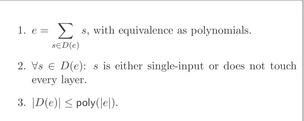
We give a decompositionD(e) of a circuite, satisfying the three properties in Figure 1.
1. e= X
s∈D(e)
s, with equivalence as polynomials.
2. ∀s ∈ D(e): s is either single-input or does not touch every layer.
3. |D(e)| ≤poly(|e|).
Figure 1: Properties of a valid decompositionD(e)
Theorem 3.4. For any circuit e whose gates each compute a graded-multilinear polynomial, there exists a poly(|e|)-time algorithm that, with probability 1−negl(|e|), outputs a decomposition D(e)
satisfying the properties in Figure 1.
For the decomposition, we view eas a layered, unbounded fan-in circuit whose layers alternate between addition (or subtraction) and multiplication gates. We further assume that all input wires to a layer come from the layer directly below, and that the top layer is a multiplication gate. Any ecan be converted to such a circuit with at most a poly(|e|) increase in size. For the remainder, we refer to the layers of eassections to avoid confusion with layers of the branching program.
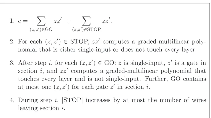
Throughout the decomposition, we maintain the invariants shown in Figure 2. We letm denote the number of sections ine, and we number the sections starting from 1 at the top, so themthsection contains e’s input variables.
1. e= X
(z,z′)∈GO
zz′ + X
(z,z′)∈STOP
zz′.
2. For each (z, z′) ∈ STOP, zz′ computes a graded-multilinear poly-nomial that is either single-input or does not touch every layer.
3. After step i, for each (z, z′) ∈GO: z is single-input, z′ is a gate in section i, and zz′ computes a graded-multilinear polynomial that
touches every layer and is not single-input. Further, GO contains at most one (z, z′) for each gatez′ in section i.
4. During step i, |STOP| increases by at most the number of wires leaving section i.
Figure 2: Invariants of the decomposition algorithm
Lemma 3.5. For any algorithm satisfying the invariants in Figure 2, upon termination the decom-position D(e) ={zz′ |(z, z′)∈ STOP} satisfies the properties in Figure 1.
Proof. We show that GO =∅aftermsteps. Then invariants 1, 2, and 4 imply the three decomposition properties, respectively.
Any gate in section mis a single-input element, and a valid product of two single-input elements is also single-input by Lemma 3.7 below. Thus, after step m GO cannot contain any (z, z′) that
satisfies the third invariant, so GO =∅.
Next, we prove Theorem 3.4. The proof uses a few simple lemmas that are proved afterwards. We will implicitly use the fact that the set of layers touched by any gate in e, and thus its input profile, can be efficiently computed (up to a 1−negl(|e|) error) using the algorithm from Lemma 2.3.
Proof of Theorem 3.4. We give anm-steppoly(|e|)-time algorithm satisfying the invariants in Figure 2. In step 1, if e is single-input or does not touch every layer, then we set GO = ∅ and STOP ={(1, e)}. Otherwise we set GO ={(1, e)} and STOP =∅.
In step i(2≤i≤m), we proceed as follows.
If section (i−1) contains multiplication gates, then at the start of stepieach (z, z′)∈GO is of
the form (z, q1×. . .×qk) for some gates q1, . . . , qk in section i. Lemma 3.8 shows that there is a
unique j∗ such that qj∗ is not single-input, and we can find this j∗ in time poly(|e|) by computing
each Prof(qj). So, we replace each (z, q1×. . .×qk)∈GO with (z×Qj6=j∗qj, qj∗). By Lemma 3.7,
we have that z×Qj6=j∗qj is single-input. Furtherqj∗ is a gate in sectioni, andz×Q
j≤kqj touches
every layer and is not single-input by the invariants on step (i−1). Finally, to ensure that there is at most one (z, z′) ∈ GO for each gate z′ in section i, we repeatedly replace any (z
If section (i−1) contains addition gates, then at the start of stepieach (z, z′)∈GO is of the form
(z, q1+· · ·+qk) for some gates q1, . . . , qk in sectioni. We first modify the expression (q1+· · ·+qk)
by zeroing any basic elements that (q1 +· · ·+qk) does not touch (in the sense of Definition 3.2),
thus ensuring that zqj is graded-multilinear for each j≤k. Then for each such (z, q1+· · ·+qk), we
remove it from GO and set
GO←GO ∪ {(z, qj) |zqj touches every layer and is not single-input}
STOP←STOP ∪ {(z, qj) |zqj does not touch every layer or is single-input}.
This adds at most one pair to STOP for each wire between layersiandi−1. Thus all invariants are now satisfied except that GO may contain multiple (z, z′) for each gate z′ in sectioni; to fix this, we again replace any (z1, z′),(z2, z′)∈ GO with (z1+z2, z′).
Next, we prove a useful structural result on multilinear polynomials, and then prove the lemmas that were used in Theorem 3.4. We use V(e) to denote the set of variables that appear in the (non-zero) monomials of the polynomial computed bye; note that this may be a strict subset of the variables at e’s input gates.
Lemma 3.6. Let e1 ande2 be arithmetic circuits computing multilinear polynomials. Ife:=e1×e2
is multilinear, then for all x∈ V(e1) and y∈ V(e2), e has a monomial that contains bothx and y.
Proof. We first show that if e is multilinear then V(e1)∩ V(e2) = ∅. If not, there is some x ∈
V(e1)∩ V(e2). Then write
e1 =x·e′1+e′′1 e2 =x·e′2+e′′2
where e′
1, e′′1, e′2, e′′2 all do not contain x and e′1, e′2 6= 0. Then because the x2 ·e′1 ·e′2 term of e is non-zero and not cancelled by any other term,e is not multilinear.
We now have that V(e1)∩ V(e2) =∅. For anyx∈ V(e1), y∈ V(e2), write
e1=x·e′1+e′′1 e2=y·e′2+e′′2
where e′
1, e′′1, e′2, e′′2 all contain neither x nor y and e′1, e′2 6= 0. Then similarly e must contain a monomial with xy.
Lemma 3.7. If e1 ande2 are graded-multilinear and single-input, and e1×e2 is graded-multilinear,
then e1×e2 is single-input.
Proof. If e1×e2 conflicts on some index j, then there are variables x1 ∈ V(e1) and x2 ∈ V(e2) that conflict on indexj, and cannot be multiplied. But by Lemma3.6,x1 andx2 appear together in some monomial, soe1×e2 is not graded-multilinear.
Lemma 3.8. Let e1, . . . , ed be graded-multilinear such that Qi≤dei is graded-multilinear, touches
every layer, and is not single-input. Then there is a unique isuch that ei is not single-input.
Proof. First note that {V(ei) |i∈[d]} gives a partition of all layers, identifying a variable with the
layer in which it appears. This is by Lemma 3.6, because any two variables from the same layer cannot be multiplied due to the index-set construction.
Pick any i such that ei is not single-input (there must be one by Lemma 3.7). Fix some index
j such that ei conflicts on j. Then ei must touch every layer that reads index j. If not, then some
other ei′ touches a matrix Cl,b1,b2 such that inpk(l) =j (for somek ∈ {1,2}), and (without loss of
generality) bk= 0, but then ei and ei′ could not be multiplied, because they conflict on index j.
If there is another value i′ 6=isuch thatei′ conflicts on indexj′6=j, then by the same argument
ei′ touches every layer that reads bitj′. But then any layer reading bothj andj′ is touched by both
Lemma 3.9. Assume z1 ×z′ and z2 ×z′ are graded-multilinear, touch every layer, and are not
single-input. If z1 and z2 are each single-input, then so is z1+z2.
Proof. Assume for contradiction that z1 and z2 are single-input butz1+z2 is not. Fix somej such that z1+z2 conflicts on index j. Then without loss of generality we have that Prof(z1)j = 0 and
Prof(z2)j = 1. As in the proof of Lemma3.8, becausez1 is single-input we must have thatz′ touches every layer that reads an index on whichz1×z′ has a conflict. Sincez1×z′ has a conflict on at least one index, and since each pair of indices are read together in at least one layer, z′ must touch some layer that reads index j. But then at least one of z1 or z2 must conflict with z′, so either z1×z′ or z2×z′ is not graded-multilinear.
3.2.2 The zero-test simulator
In this section we describe and analyze the simulator Sim0 that is used to answer a single zero-test. Recall that an element e is an arithmetic circuit computing a polynomial whose variables are the entries of Ci,b1,b2 fori∈[n], b1, b2 ∈ {0,1}. However, as Ci,b1,b2 =αi,b1,b2 ·B˜i,b1,b2, we can think of it
as a polynomial in theαi,b1,b2, with coefficients that are polynomials in the entries of ˜Bi,b1,b2. Under
this viewpoint, we refer to the monomials as “α-monomials”. We associate an index-set with each αi,b1,b2 and each entry of ˜Bi,b1,b2, namely the index-set of Ci,b1,b2.
Definition 3.10. We say that a monomial in the variables {αi,b1,b2 : i∈[n], b1, b2 ∈ {0,1}} is full
if it contains, for everyi∈[n], exactly one of the α’s of layeri(i.e., one of αi,0,0, αi,0,1, αi,1,0, αi,1,1).
Notice that ife is graded-multilinear then everyα-monomial contains at most one α from every layer, because the index-sets of every pair of layer-i α’s intersect and so they cannot be multiplied. We need the following simple observation:
Lemma 3.11. Let ebe an arithmetic circuit whose gates each compute a graded-multilinear polyno-mial and let D(e) be its decomposition given by Theorem 3.4. Then each s∈D(e) contains at most one full α-monomial, and each of e’s fullα-monomials appears in exactly one s∈D(e).
Proof. We may assume without loss of generality that each single-input element inD(e) has a unique profile, by replacing anys6=s′ ∈D(e) such thatProf(s) =Prof(s′)6=⊥withs+s′. Then the lemma holds because (1) any element that does not touch every layer cannot contain a fullα-monomial, and (2) any single-input element swith a complete profile can only contain the unique full α-monomial corresponding toProf(s). (Note that (1) includes single-input elements with incomplete profiles.)
Given an element s that contains at most one full α-monomial, we can extract it (if it exists) by computing the homogeneous degree-n portion of susing the algorithm from Lemma2.1. This is because due to the index-set construction, the only possible monomials of degree n are the full α-monomials. Further, we show in Lemma3.16below that for any elementswithnofullα-monomials, with high probabilitysevaluates to 0 on the obfuscation iff it computes the identically 0 polynomial. The final ingredient we need is a method of sampling an assignment to the variables of a full α-monomial that is indistinguishable from the corresponding marginal distribution of the obfuscation. We use the method of [AGIS14, Thm. 7]. (Recall that randBPwas defined in Section 2.6.)
Theorem 3.12 ([AGIS14]). Let BP be an oblivious dual-input RMBP that computes F :{0,1}ℓ → {0,1}, and letBP′:=randBP(BP). There exists a PPT simulatorSim′ such that for everyx∈ {0,1}ℓ,
BP′|x ≡Sim′ 1|F|, F(x) .
Construction 3.13 (Zero-test simulator). The zero-test simulator Sim0 uses the decomposition algorithm Dof Theorem 3.4. On input e,Sim0 operates as follows.
1. Compute the decomposition D(e).
2. For every single-input element s ∈D(e) with a complete profile, use Lemma 2.1 to construct an element αes that computes the homogeneous degree-n portion of s. (Ifsis not single-input
or has an incomplete profile, defineαes:= 0.)
3. For every single-input element s∈D(e) with a complete profile, zero-test αes as follows: query
the oracleF onx :=Prof(s), and evaluate αes on Sim′ 1|C|, C(x)
, whereSim′ is the simulator of [AGIS14, Thm. 7]. If any such evaluation is non-zero, stop and return “e6= 0”.
4. Construct the element e′ := e−P
s∈D(e)αes, and test if e′ computes the identically zero
poly-nomial using Schwartz-Zippel. If so then return “e= 0”, otherwise return “e6= 0”.
Construction 3.13 runs in time poly(n) because each step does. The following theorem shows its correctness, and completes the proof of Theorem 1.6. We use Vreal to denote the real-world distribution of the obfuscated program.
Theorem 3.14. Let e be an arithmetic circuit whose gates each compute a graded-multilinear poly-nomial, and let Sim0 be as in Construction 3.13. Then PrSim0(e) = 0−Prv←Vreal[e(v) = 0]
=
negl(n), where the probabilities are over the randomness of Sim0 and the obfuscator.
Proof. Lemma 3.15 shows that for any such e, if e(Vreal) 6≡ 0 then Pr
v←Vreal[e(v) = 0] = negl(n). (This is proved exactly as in [BGK+14].) Thus it suffices to prove that, with high probability over
its randomness, Sim0 returns “e = 0” iff e(Vreal) ≡ 0. Observe further that e(Vreal) ≡ 0 if and only if α(e Vreal) ≡ 0 for every α-monomial αe in e. The “if” direction is clear; for the “only if” direction, assume that someα-monomials are not identically zero onVreal. Then for some sample of the marginal distribution on {Bei,b1,b2}i,b1,b2, e becomes a non-zero polynomial in just the variables {αi,b1,b2}i,b1,b2. Then since the marginal distribution on this latter set is uniform conditioned on any
sample of{Bei,b1,b2}i,b1,b2, there is some sample v← V
real for whiche(v)6= 0, and thuse(Vreal)6≡0.
We now show that, with probability 1−negl(n) over its randomness,Sim0 returns “e= 0” iff all α-monomialsαe inesatisfyα(e Vreal)≡0.
Assume that e contains some fullα-monomial αes such thatαes(Vreal) 6≡0. We claim that, with
probability 1−negl(n) over the randomness of Sim0, step 3 in Construction 3.13 returns “e 6= 0”. Indeed, because the call to Sim′ generates exactly the marginal distribution on αes’s variables by
Theorem 3.12, the evaluation generates a sample from αes(Vreal). By Lemma 3.15 this evaluation is
non-zero with probability 1−negl(n) becauseαes(Vreal)6≡0, and thus step3 returns “e6= 0”.
Now assume that every full α-monomialαessatisfiesαes(Vreal)≡0. ThenSim0 reaches step4with
probability 1. Notice that e′ contains exactly the non-full α-monomials in e. We show in Lemma 3.16that e′ computes the identically zero polynomial iff each of its α-monomials is 0 onVreal. Thus, with probability 1−negl(n) over the randomness ofSim0, step4returns “e= 0” iff each α-monomial
e
α inesatisfiesα(e Vreal)≡0.
We now state the lemmas used in Theorem3.14. The first is [BGK+14, Claim 8]; for completeness
we include a proof in AppendixA.
Lemma 3.15 ([BGK+14]). For any valid element e, if e(Vreal) 6≡ 0 then Pr
v←Vreal[e(v) = 0] = negl(n).
Lemma 3.16. If e contains no full α-monomials, then it is the identically zero polynomial iff
e
α(Vreal)≡0 for every α-monomial αe in e.
Proof. The “only if” direction is clear. For the “if” direction, we show that for any individual non-full α-monomial α,e α(e Vreal)≡0 iffαeis identically zero (i.e. if its coefficient is identically zero).
Fix any non-full α-monomial α. We first show that the marginal distribution on the variablese
of {s,˜ ˜t,B˜i,b1,b2 | i ∈ [n], b1, b2 ∈ {0,1}} that appear in α’s coefficient consists of uniform non-zeroe
vectors and uniform non-singular matrices. LetC ⊆nCi,bi
1,bi2 : i∈[n], b
i
1, bi2∈ {0,1}
o
denote the set of matrices from which α’s variables come. Notice thate C contains at most one matrix from every layer of the RMBP, because ifCi,b1,b2 ∈ B thenαi,b1,b2 appears in the monomialα, bute αe contains at
most one αi,b1,b2 from every layer i. Let I ⊂ [n] denote the layers from which C contains a matrix,
and let B=nB˜i,bi
1,bi2 : Ci,bi1,bi2 ∈ C o
. Then the marginal distribution of Vreal on ˜s, ˜t, and Bis
˜
s = e1·R−01 ˜
Bi,bi
1,bi2 = Ri−1·Bi,bi1,bi2 ·R −1
i , ∀i∈ I
˜
t = Rn·ew
where each Bi,bi
1,bi2 ∈
Zw×w
p is a fixed non-singular matrix, and each Ri ∈ Zwp×w is a uniform
non-singular matrix. As noted above, there is at most one Ci,bi
1,bi2 ∈ C for each i ∈ I, i.e., at most one
˜ Bi,bi
1,bi2 on whichαe depends, for everyi∈ I. Consequently, the random matrices{Ri |i= 0, . . . , n}
can be assigned to these equations in a way so that at most one random matrix is assigned to each equation. (This is because |I| < n because αe is not a full monomial, and thus there are ≤ n+ 1 equations and there aren+ 1 random matrices.) Thus, the left-hand side of each equation is uniform in its support, even conditioned on any fixing of the other left-hand sides. Since the supports are all non-singular matrices (or all non-zero vectors in the case of ˜s and ˜t), we have that when restricted to these values, the distribution we have generated is identical toVreal.
Let Vrand denote the distribution over assignments to the variables of α, when ˜e s,˜t are replaced with uniform vectors us, ut, and the matrices in B are replaced with uniformly random matrices
M1, ..., M|I|. Because Pru←Zw p [u6= 0
w] = 1−p−w = 1−negl(n), and because a uniform matrix in
Zwp×w is non-singular with probability≥1−w/p= 1−negl(n), the distributionsus, ut, M1, ..., M|I|
andns,˜ t,˜B˜i,bi
1,bi2 ∈ B o
arenegl(n)-close in statistical distance. Thus because applying a deterministic function to random variables does not increase the statistical distance, we have
v←VPrreal[αe(v) = 0]−v←VPrrand[αe(v) = 0]
=negl(n). (1)
If α(e Vreal)6≡0 then clearlyαeis not the zero polynomial. If on the other hand α(e Vreal)≡0, then (1) implies Prv←Vrand[αe(v) = 0] = 1−negl(n). Thus because deg(α)e < n, the Schwartz-Zippel lemma implies thatαe is the zero polynomial.
4
Security for unrestricted graded encoding schemes
As before, the difficulty is in simulating zero-test queries. By definition in this model, IsZeroonly returns True on circuits that compute graded-multilinear polynomials. Because we can efficiently test for graded-multilinearity as described in Section 3.1, we can restrict ourselves to such circuits.
Throughout this section we let me denote the number of full α-monomials (in the sense of Def.
3.10) for a given circuit e. In Section 4.2 we give an algorithm for simulating zero-test queries that runs in time poly(me,|e|). Thus if every graded-multilinear polynomial computed by a
polynomial-size circuitecontains a polynomial number of fullα-monomials, this algorithm gives a VBB simulator (and, in any case, the algorithm gives an iO simulator).
In Section 4.1 we show that a polynomial bound on me follows from a new hypothesis which
is closely related to a parameterized version of the Bounded Speedup Hypothesis introduced by Brakerski and Rothblum [BR14a,BR14b] (see that section for further discussion). Thus under this new hypothesis we can achieve VBB security.
However, we first show that unconditionally obtaining a VBB simulator in this model for any algebraic obfuscator would imply the algebraic analog of P 6= NP, namely VP 6= VNP. Intuitively, this is because the polynomial summing a function’s outputs over all possible inputs is in VNP, but this polynomial cannot in general be simulated with only black-box access. This is formalized in the proof of Theorem 1.7below; we first state some definitions.
Definition 4.1 (VP [Val79]). Let m(n) = poly(n). A familyF =fn:{0,1}m(n) → {0,1} n is in
VP if for every n, deg(fn) = poly(n), and there exists a polynomial p(n), and a family {Cn}n of
arithmetic circuits such that for any n,|Cn| ≤p(n), andCn(x) =fn(x) for every x∈ {0,1}m(n).
Definition 4.2 (VNP [Val79]). Let m(n), k(n) = poly(n). A family F =
fn:{0,1}m(n)→ {0,1} n is in VNP if there exists a family G =
gn:{0,1}m(n)+k(n)→ {0,1} n
in VP such that, for everynand every x∈ {0,1}m(n),f
n(x) =Py∈{0,1}k(n)gn(x, y).
Definition 4.3 (Algebraic obfuscator). An algorithm O that takes as input a circuit f :{0,1}n → {0,1}is analgebraic obfuscatorifO(f) = ({ki}i, E), where (1){ki}iis apoly(|f|)-size set of encodings
in some GES, (2)Eis apoly(|f|)-size arithmetic circuit, and (3) for everyx∈ {0,1}n, the computation
ofE({ki}i, x) obeys the restrictions of the GES and satisfiesIsZero(E({ki}i, x)) = True ifff(x) = 0.
Theorem 1.7. If there exists a polynomial-time algebraic obfuscator that achieves VBB security for all NC1 circuits in the unrestricted ideal GES model, then VP6= VNP.
Proof. Assume the existence of an obfuscator Oas in the theorem statement, that on input a circuit to be obfuscated outputs an evaluation circuitE, and a set{ki}iof encodings (namely,Oinstantiates
the unrestricted ideal GES oracle with these encodings). We use O to construct a function family
F ∈ VNP\VP. For every n ∈ N, let Cn :{0,1}n → {0,1} be the circuit that always outputs 0; and for every xn0 ∈ {0,1}n, let C
xn
0 :{0,1}
n → {0,1} be the circuit that outputs 1 only on xn 0, i.e., Cxn
0 (x
n
0) = 1, and for every xn0 6=x ∈ {0,1}n, Cxn
0 (x) = 0. Let C ={Cn}n∈N∪ {Cx0n}n∈N,xn0∈{0,1}n,
and assume that for everyn∈Nand xn
0 ∈ {0,1}n,|Cn|= Cxn
0
. (This is without loss of generality, since all circuits takingn-bit inputs can be padded to have the same size as the circuit with maximal size.) For every n ∈ N, let fn({ki}) = P
x∈{0,1}nE({ki}i, x), and F = {fn}, then F ∈ VNP by
definition. We show that F ∈/ VP, by showing that a PPT simulator cannot simulate zero-test queries to fn({ki}), where {ki} are the encodings in an obfuscation of a circuit from the family C.
Indeed, if such zero-test queries cannot be simulated then the VBB property of O guarantees that no polynomial-time adversary can construct circuits computing the functions fn, namely F has no
polynomial-sized circuits.