Detection of global runoff changes: results from observations and CMIP5 experiments

(1)

Hydrol. Earth Syst. Sci., 17, 2967–2979, 2013 www.hydrol-earth-syst-sci.net/17/2967/2013/ doi:10.5194/hess-17-2967-2013

EGU Journal Logos (RGB)

Advances in

Geosciences

Open Access

Natural Hazards

and Earth System

Sciences

Open Access

Annales

Geophysicae

Open Access

Nonlinear Processes

in Geophysics

Open Access

Atmospheric

Chemistry

and Physics

Open Access

Atmospheric

Chemistry

and Physics

Open Access Discussions

Atmospheric

Measurement

Techniques

Open Access

Atmospheric

Measurement

Techniques

Biogeosciences

Open Access Open Access

Biogeosciences

Discussions

Climate

of the Past

Climate

of the Past

Discussions

Earth System

Dynamics

Earth System

Dynamics

Discussions

Geoscientific

Instrumentation

Methods and

Data Systems

Open Access

_{Geoscientific}

Instrumentation

Methods and

Data Systems

Geoscientific

Model Development

Geoscientific

Model Development

Discussions

Hydrology and

Earth System

Sciences

Open Access

Hydrology and

Earth System

Sciences

Ocean Science

Discussions

Solid Earth

Discussions

The Cryosphere

Discussions

Natural Hazards

and Earth System

Sciences

Open Access

Discussions

Detection of global runoff changes:

results from observations and CMIP5 experiments

R. Alkama, L. Marchand, A. Ribes, and B. Decharme

Groupe d’étude de l’atmosphère météorologique (GAME), UMR3589, CNRM/GAME – Météo-France, Toulouse, France

Correspondence to: R. Alkama ([email protected])

Received: 24 January 2013 – Published in Hydrol. Earth Syst. Sci. Discuss.: 19 February 2013 Revised: 6 June 2013 – Accepted: 21 June 2013 – Published: 25 July 2013

Abstract. This paper assesses the detectability of changes in global streamflow. First, a statistical detection method is applied to observed (no missing data which represent 42 % of global discharge) and reconstructed (gaps are filled in order to cover a larger area and about 60 % of global dis-charge) streamflow. Observations show no change over the 1958–1992 period. Further, an extension to 2004 over the same catchment areas using reconstructed data does not pro-vide epro-vidence of a significant change. Conversely, a signif-icant change is found in reconstructed streamflow when a larger area is considered. These results suggest that changes in global streamflow are still unclear. Moreover, changes in streamflow as simulated by models from Coupled Model In-tercomparison Project 5 (CMIP5) using the historic and fu-ture RCP 8.5 scenarios are investigated. Most CMIP5 models are found to simulate the climatological streamflow reason-ably well, except for over South America and Africa. Change becomes significant between 2016 and 2040 for all but three models.

1 Introduction

Human influence has now been documented in several parts of the water cycle: atmospheric water vapour (e.g. Willett et al., 2007; Santer et al., 2007), land precipitation (e.g. Zhang et al., 2007), or land evapotranspiration (e.g. Douville et al., 2013). The case of runoff or river discharge is more con-trasted. While some studies thought to have identified robust trends over some specific regions (e.g. Stahl et al., 2010 over Europe, Krakauer and Fung, 2008 over the US), other stud-ies focused on the global scale have led to somewhat contra-dictory results. Based on 221 rivers, corresponding to 40 %

of global continental runoff, Labat et al. (2004) documented an increasing global runoff at the end of the 20th century compared to the beginning. In contrast, based on data from 925 rivers, corresponding to 80 % of global runoff, Dai et al. (2009) show a slight decrease in global runoff over the second half of 20th century. This discrepancy can be ex-plained by the differences either in the number of gauging stations used, in the period of investigation, or in the method used to fill the gaps. Indeed, both studies were using some reconstructions (meaning gap filling) in order to provide a more comprehensive spatio-temporal coverage.

(2)

in most LSMs, could have contributed to increased runoff at high latitude. They also emphasize that runoff trend is a regional scale issue, if not basin dependent. Finally, the ma-jority of recent studies conclude that there was no significant global runoff trend in the late twentieth century (Milliman et al., 2008; Dai et al., 2009; Alkama et al., 2011).

This paper first aims to provide a novel assessment of the significance of recent observed changes. This assessment is based on the temporal optimal detection (TOD) method (Ribes et al., 2010). While most previous studies consider global mean runoff, the TOD method is able to provide a single global diagnostic based on continental-scale mean runoffs. The TOD method is applied to both observed data only (meaning no missing data) and reconstructed data (i.e. a substantial fraction of streamflow time series is missing and reconstructed by Dai et al., 2009).

With regard to future projections, an intensification of the hydrological cycle over the 21st century is widely assumed (e.g. Liu et al., 2012). However, regional patterns of human-induced changes in surface hydroclimate are complex and less certain than those in temperature. Indeed, both increases or decreases may be expected in future precipitation and runoff, depending on the region (Milly et al., 2005; Alkama et al., 2010). Our study investigates the large-scale runoff change over the late 20th and 21st century (with atmospheric greenhouse gas and aerosol concentrations from the Repre-sentative Concentration Pathways RCP 8.5 scenario), as sim-ulated by 14 CMIP5 (http://cmip-pcmdi.llnl.gov/cmip5/) At-mosphere Ocean General Circulation Models (AOGCMs). First, we assess the extent to which these simulated runoffs are consistent with observations. To this end, a compari-son with observed streamflow is performed for the past few decades. Second, the same experiments are used to investi-gate how the anthropogenic perturbation (green house gases) may lead to different responses, depending on the model. Third, the same detection technique is applied to climate change scenarios in order to determine the significance of the simulated changes. The date at which the changes be-come significant is of particular interest, and provides some information with respect to the consistency or inconsistency between observed and simulated changes.

This paper primarily addresses the following three major issues:

1. How does global observed and reconstructed stream flow change over time?

2. Are simulated streamflows reasonably consistent with observations?

3. How will streamflow change in the future?

2 Methodology

2.1 Data

To the best of our knowledge, the most complete down-stream discharge dataset in existence was collected by Dai et al. (2009). This dataset represents historical monthly stream-flow at the farthest downstream stations for the world’s 925 largest ocean-reaching rivers from 1900 to 2004. However, the length and reliability of the available time series vary greatly from one river basin to another, and gaps are usually found. Observed streamflows are subject to some uncertain-ties, and in particular measurement uncertainty (e.g. related to the estimation of rating curves), potential homogeneity breaks, and missing values. Measurement errors are very dif-ficult to address and no homogenised datasets are currently available, so the results provided in this study are conditional to this dataset, following previous work (e.g. Dai et al., 2009) that also investigated the recent trends in global streamflows. Gaps may be filled by using statistical techniques, numerical simulations using land surface models (LSMs), or a combi-nation of both. In the present application, gaps were filled by applying a statistical linear correction to the river dis-charge simulated by a LSM with observed atmospheric forc-ings (see Dai et al., 2009). Such a reconstruction, however, is likely to introduce additional uncertainty. Results may de-pend on potential inaccuracy of the LSM used, homogeneity breaks in the atmospheric forcing, uncertainties coming from the observations (sometimes only a few years) used to cali-brate the statistical correction, and others. As a consequence, this study carefully distinguishes between two different treat-ments. First, we analyse observed streamflows only, by con-sidering time series with no missing data. In this way, the number of the selected rivers is reduced to 161 over 1958– 1992 period. This period was chosen in order to find an op-timal compromise between spatial and temporal covering. Note that even under this restrictive treatment, the period investigated is similar to the one considered in Gedney et al. (2006) or Alkama et al. (2010). Second, in order to con-sider the larger spatio-temporal coverage available, we ap-ply the same analysis to the dataset including reconstructed streamflows. As linear regression cannot be used if there is too much missing data, Dai et al. (2009) succeeded in re-constructing only 687 gauging stations for the whole 1958– 2004 period. We consider these 687 catchment areas over this period. Finally, a third product is used in order to ex-tend the “observations” up to 2004. We then consider the 161 rivers observed over the 1958–1992 period and allow miss-ing/reconstructed values over the 1993–2004 period. This ex-tension does include reconstructions, but the amount of re-constructed values is much reduced compared to the previous case (i.e. 687 rivers).

(3)

(dams), water withdrawal (e.g. irrigation, industrial or do-mestic uses), changes in land use that impact evapotranspira-tion, and others. In terms of climate change detection attribu-tion, these direct influences may be regarded as “confound-ing factors”, as they may cause a substantial trend without any climate change. Detailed estimation of such direct pertur-bations is very challenging and no global discharge database of “naturalized streamflows” is currently available. However, several studies addressed the issue of quantifying these direct anthropogenic influences at the global scale, and suggested that they had a minor impact on multi-year trends.

Wisser et al. (2010), have quantified the impact of irri-gation and reservoir operations over the 20th century. They concluded that “the land use, expansion of irrigation and the construction of reservoirs has considerably and gradually im-pacted hydrological components in individual river basins. Variations in the volume of water entering the oceans an-nually, however, are governed primarily by variations in the climate signal alone with human activities playing a minor role”. The later is shown to hold at the continental scale (i.e. for individual oceanic basin, which corresponds to scales similar to the ones considered here, but with a different clus-tering). Other studies (e.g. McCelland et al., 2004; Adam et al., 2007; Adam and Lettenmaier, 2008) confirmed that dams have altered the seasonality of discharge, especially over up-stream rivers, but are not responsible for changing annual values. Then, the impacts of land use changes on land sur-face hydrology are still debated. On the one hand, when irri-gation is neglected, land use can have an important influence on runoff via a decrease in surface evapotranspiration (Piao et al., 2007). This conclusion is also supported by Sterling et al. (2013) in the case of taking into account the irrigation. On the other hand, Liu et al. (2008) and Sun et al. (2008) indi-cate that deforestation over China, associated with irrigation, leads to increased evapotranspiration over the 20th century. Other studies, over individual river basins, suggested that the sign of land use induced change was unclear (e.g. Twine et al., 2004, over the Mississipi river basin, VanShaar et al., 2002, over the Columbia River basin). Finally, some direct human influences via other activities have also been investi-gated and shown to have limited impact. For instance, Mc-Celland et al. (2004) demonstrated that increased forest fire frequency and severity may have contributed to changes in discharge, but cannot be considered as a major driver.

We also used simulated runoff by different models from to the Coupled Model Inter-comparison Project Phase 5 (CMIP5). Those runs supply three kinds of experiments: his-torical runs in which all external forcings come from obser-vations, future runs which use greenhouse gas and aerosol emissions from the RCP 8.5 scenario, and finally piControl runs in which pre-industrial forcings are constant. The pi-Control runs are used to evaluate the internal climate vari-ability. There are four RCPs types of possible future scenar-ios, and the RCP 8.5 involves the highest greenhouse gas concentrations at the end of the 21th century. It expects to

reach the radiative forcing of 8.5 W m−2 (∼4 times more than the current value) at the end of 2100 which correspond approximately to 1370 ppmv of atmospheric CO2 concentra-tion. This scenario involves an intensive use of fossil fuels, with little mitigation stringency.

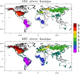
For this entire study, an ensemble of 8 zones where river basins are merged by continent and climate area was se-lected. The motivation for separating the northern cold cli-mate from the tropics comes from Dai et al. (2009) and Alkama et al. (2011), which found significant runoff increase at high latitude that cannot be explained by the atmospheric forcing. While the motivation of merging all of Africa’s river basins in a single zone, even with the existence of large dif-ferences in climates, is coming from an ensemble of previous studies that shows that generally all of the largest African river basins had significantly decreased over the second half of 20th century (e.g. Alkama et al., 2011; Dai et al., 2009; Gedney et al., 2006; Labat et al., 2004). The 8 selected zones are North America, Central America, South America, North Europe (including arctic basins), South Europe, North Asia (corresponding to Siberia), South Asia (including Oceania) and Africa (Fig. 1).

Three steps are used before comparing the modelled runoff by different CMIP5 experiments and observations over the 8 regions: (1) interpolate using bilinear method all of the CMIP5 modelled runoff (mm d−1) into the same grid (0.5◦×0.5◦); (2) aggregate the river basins at the 0.5◦×0.5◦ grid. To be consistent with the data, river basins are defined at the known latitude and longitude of the observed gauged stations which are different to the river mouth; (3) simulated runoff are then averaged over the computed river basins and merged into the 8 defined zones in the Fig. 1.

2.2 Statistical method

2.2.1 The temporal optimal detection method

Detection is the process of demonstrating that an observed change is significantly different (in a statistical sense) that cannot be explained by natural internal variability. The sta-tistical method used for detection is the temporal optimal de-tection method (Ribes et al., 2010). We review the main con-cepts here but refer to Ribes et al. (2010) for full details about the method. The TOD method is based on a linear model:

(4)

[image:4.595.128.469.64.379.2]

Fig. 1. Coverage of 161 (687) river basins top (bottom) over the 8 selected zones which are 1 = South America, 2 = Africa, 3 = South Asia including Oceania, 4 = North Asia corresponding to Siberia, 5 = South Europe, 6 = North Europe including Arctic basins, 7 = Central America and 8 = North America. The circles represent the in situ gauged stations for each river accounted for in this study.

This assumption makes the TOD method particularly suit-able here, because the spatial pattern of changes in global runoff is still under debate and somewhat model-dependent (see Sect. 3.2).

Regarding internal variability, the TOD method assumes thatεhas a red noise structure (or autoregressive process of order 1, AR1, see e.g. Brockwell and Davis 1991). The red noise structure means that the random termε(s, t )satisfies: ε(s, t )=αε(s, t−1)+η(s, t ), (2) whereη(s, t ) is a white noise in time, i.e. η(s, t ) is inde-pendent fromη(s, t−1). This assumption also means that, for example, the autocorrelation function decreases exponen-tially, with no long-range memory effect. An AR1 process is then described by a single parameter,α(see Eq. 2), which is the one-year lag autocorrelation ofε. Note that in many statistical tests, residuals ε are assumed to be white noise (i.e.α=0), which makes the detection easier.

GivenY (s, t ),x(t )andα, the inputs, the TOD method pro-vides an estimate of the trend at each locationb(s). Based on this estimate, TOD performs a statistical test of the null-hypothesis “b=0”, and so returns a single P value describ-ing how significantly observations have changed.

2.2.2 Application to global runoff data

Here we discuss the choice of the parametersx(t )andα, and the extent to which global discharges satisfy the assumptions behind the TOD method.

While assumed to be known, the temporal pattern of changex(t )is commonly evaluated from simulations. In or-der to base our study on a very simple temporal pattern that is not model-dependent, we used only linear trends (i.e.x(t )= t). Note that the use of a linear trend instead of a potentially more complex smooth temporal pattern may be suboptimal. However, over short periods like the ones investigated here for observation (35 or 45 yr) the non-linearity of the change is probably not the dominant feature. In addition to be very simple, this choice is consistent with several previous studies dealing with potential changes in global hydrology (e.g. La-bat et al., 2004; Gedney et al., 2006; Dai et al., 2009; Alkama et al., 2010, 2011).

(5)

Fig. 2

Fig. 2. (a) estimated alpha (α) based on the global runoff time series from each CMIP5 model (piControl simulations); (b), (c) and (d) are the distribution of the P value when TOD test is applied to different segments of 50 yr periods of all CMIP5 control runs usingα=0, 0.2 and 0.3, respectively.

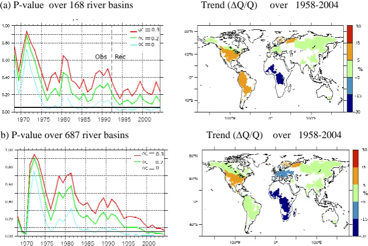
(a) P-value over 168 river basins Trend (∆Q/Q) over 1958-2004

(b) P-value over 687 river basins Trend (∆Q/Q) over 1958-2004

Fig. 3

[image:5.595.116.481.66.334.2] [image:5.595.116.481.394.638.2]

(6)

control simulations where external forcings are constant over time are expected to provide a physically based description of internal variability, and using such simulations is quite common in detection and attribution studies (e.g. Hegerl and Zwiers, 2011). Figure 2a shows theαvalue as estimated from the time series of global runoff, for each CMIP5 control sim-ulation. It is computed as the correlation betweeny(t ) and y(t−1). Although some discrepancies appear between dif-ferent models, all values are between 0.04 and 0.3 with a medium value close to 0.2. These control simulations may also be used to check the accuracy of the red noise assump-tion. Figure 2b, c and d illustrate the distribution of the P value if the TOD test is applied to different 50 yr segments from all control simulations usingα=0, 0.2 or 0.3, respec-tively. Such segments could be regarded as independent re-alizations under the null distribution of the test. If internal variability is properly accounted for (in particular, if the red noise assumption is accurate), the P values of the test ap-plied to these segments should be distributed uniformly be-tween 0 and 1. Figure 2b, c and d suggests that the more suit-able choice isα=0.2 (distribution close to uniform), while α=0.3 (resp.α=0) is too conservative (permissive), lead-ing to less (more) than expected values under the 5 % thresh-old. In the following, we primarily discuss the results assum-ingα=0.2 orα=0.3 (which makes the detection more con-servative and corresponds to the highest value found in indi-vidual models). The results obtained withα=0 (i.e. white noise) are also shown in some cases in order to provide a lower bound where no memory effect is accounted for. Note that the red noise assumption withα=0.2 seems also con-sistent with the autocorrelation function of streamflow, as simulated in control runs (not shown).

Finally, an important feature of the method with respect to our study is that it performs a multivariate diagnosis; i.e. it provides one single statistical diagnosis based on regional (continental-scale) streamflow. In particular, a change that generates increases or decreases in runoff depending on the region would be captured by this method. The TOD method, as implemented here, may then be regarded as a strategy for testing trends significance that allows the change to be spa-tially non-uniform and takes into account a non-white inter-nal variability. In particular, it differs from testing the signif-icance of each regional trend individually, as a single test is performed for all regions simultaneously here.

3 Results

3.1 Statistical test on observed and reconstructed runoffs

The coverage of the 161, respectively 687, rivers worldwide is shown in Fig. 1. Some regions (e.g. western part of Asia, desert regions and southern part of South America) suffer from lack of data. Indeed, only 31 % (43 %) of global land

area excluding Antarctica are covered by the 161 (687) rivers basins which correspond to about 42 % (60 %) of global land discharge.

We first applied the TOD method to observed runoff over the 1958–1992 period, based on 8 zones in which observed streamflow at 161 downstream gauged stations are merged. Results are shown in Fig. 3a in terms of P value, for three values of the α coefficient. The P value of year 1980, for instance, is obtained by applying the test to the data before 1980, i.e. the 1958–1980 period. This allows us to analyze the time evolution of the P value. The P value shown in 1992 provides the result of the statistical test applied to the full pe-riod of interest, 1958–1992. As might have been expected, larger year-to-year variations are observed at the beginning of the period compared to the end, as one single year has a stronger relative impact on the P value (the size of the sample being smaller). This paper also investigates the date at which detection occurs. A precise definition of this date is then re-quired. In the following, we consider that detection occurs on year “t0” if the P value of the statistical test (TOD method) remains below the 5 % threshold aftert0 (i.e. for allt > t0), while it was higher than 5 % the year before (i.e.t0−1). Note that using such a definition, the P value might have fallen below 5 % at some datet1< t0 (but the significance of the change has then vanished at some point betweent1 andt0).

Figure 3a (left) shows that the P value remains higher than the significance threshold, 0.05, over the 1958–1992 period. This reveals no significant change in observed streamflow until 1992. This result is very robust here as it is obtained even under the white-noise (i.e.α=0 which is very unlikely) assumption.

(7)

[image:7.595.112.485.66.400.2]

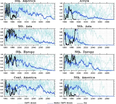
Fig. 4. Temporal P value of observed (black) and simulated (light blue) runoff over the 8 regions merging 161 river basins usingαat 0.2. The median of the 14 is in blue.

In the same way, TOD is applied over the 687 river basins and over the same period (1958–2004). Figure 3b shows a significant change in reconstructed runoff since 2000 at the 95 % significance level forα=0 and, to a lesser extent, for α=0.2. Forα=0.2, the P value remains below but close to the significance level of 5 %. Forα=0.3, no changes are found. Here, we conclude that a change is detected, because detection does occur with a medium value ofα. This result is not very robust, however, as detection no longer holds with a more conservative choice of α. Taking into account new rivers (687 rather than 161) and/or reconstructed rather than observed streamflow then seems to impact the results. How-ever, the distribution and intensity of the relative discharge anomaly are not notably affected (Fig. 3b). Africa is still the only region that exhibits a significant (negative) runoff trend.

3.2 Evolution of observed and simulated runoff

The evaluation of the CMIP5 simulated runoff was per-formed over the 8 zones and at the global scale corresponding to the 161 river basins. Figure 5 shows the temporal evolu-tion of the yearly mean runoff (mm d−1) from 1958 to 2100

(8)

[image:8.595.98.494.65.419.2]

Fig. 5. From 1958 to 2100 global and regional time series of the simulated (colours) and observed (black) annual runoff. The median of the fourteen models is given by the thick red line.

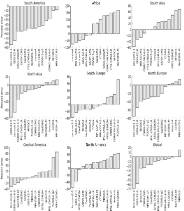
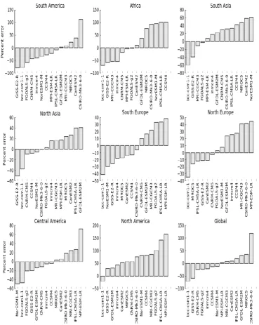
simulated (Fig. 7). Indeed, it did not exceed 50 % except over Africa (North America) where only CNRM, MPI, FGOALS, CanESM and GFDL (GFDL and INM) are reasonable. We can also note the large error of CSISRO (MPI) over South America (Centrale America).

Over the same period 1958–1992, observations show a large 0.05 mm yr−2 positive (negative) runoff trend over South America (Africa), only reproduced by MRI and MIROC (FGOALS and MIROC; Fig. 8). Remaining models exhibit small or opposite trends. Over all regions, the models did not show any consensus with respect to the 1958–1992 trend. In particular, the sign of the trend depend on the model, some models are close to the observed trend while others do not, etc. Many conclusions drawn from the previous CMIP3 exercise (e.g. Milly et al., 2005; Nohara et al., 2006) were consistent with the present study in terms of the comparison between simulated and observed runoff means, inter-annual variability and trends. Despite the different bias existing in different model simulation, no bias correction methods are applied in this study.

(9)

R. Alkama et al.: Results from observations and CMIP5 experiments 2975

Fig. 6

Fig. 6. Percent error (100(Sim-Obs)/Obs) of simulated runoff averaged over the 1958–1992 period.

3.3 Statistical test on simulated runoff

In Fig. 9, the TOD test is applied to each CMIP5 model over the 161 global river basins still merged into 8 zones, and over the whole 1958–2100 period. In order to highlight central behaviour, the median of these 14 P values is com-puted each year, and its time evolution is illustrated. The P values are also shown for the observed and the reconstructed data previously presented. Note that the P values of observed and simulated runoff are calculated over the 161 river basins whereas reconstructed data are computed over the 687 river basins. The P values obtained from the CMIP5 runoff cal-culated over the 687 rivers are very similar to those com-puted over the 161 rivers. The results are only shown for α=0.2 (medium value). We define the date at which

detec-tion occurs as the first year for which the P value remains lower than the 0.05 threshold up to 2100. The two models that simulate low runoff variability, BCC and GISS, are the first to detect a significant runoff change (in 2002 and 2005, respectively). The INM model, simulating no global signifi-cant trend, is the last to detect a signifisignifi-cant change, in 2060. All other models detect a significant change between 2016 and 2040. This means that changes in runoff, as simulated by current climate models, are expected to become significant in the coming decades. As a consequence, the result previously obtained on observed runoff (161 river basins) appears to be very consistent with climate model projections.

[image:9.595.113.483.61.484.2]

(10)

Fig. 7

Fig. 7. Percent error (100(Sim-Obs)/Obs) of the standard deviation runoff simulated by CMIP5 models over the 1958–1992 period.

value computed from reconstructed runoff is on the border (if not outside) of the set of climate model projections. This feature, together with the substantial difference between the results obtained on observed and reconstructed data, may call into question the quality of reconstructions, and/or the accu-racy of climate model projections.

The results from the same analysis applied over individ-ual regions is shown in Fig. 4. Similarly to what was found at the global scale, the P values are very scattered over the 20th century, and tend to become closer at the end of the 21st century. This analysis suggests that the detection oc-curs earlier in northern high latitude regions, consistent with

[image:10.595.114.484.60.524.2]

(11)

Fig. 8

Fig. 8. Observed and simulated runoff trends over the 1958–1992 period.

4 Summary and conclusions

In this work, the TOD statistical test (Ribes et al., 2010) is used to evaluate the possible changes on recent and future (RCP 8.5 conditions) runoff, based on fourteen CMIP5 ex-periments and streamflow data from Dai et al. (2009). This evaluation is made over 8 zones, merging the world’s 161 largest rivers. Our analysis suggests some answers to the three issues raised in the Introduction.

4.1 How does global observed and reconstructed streamflow change over time?

[image:11.595.116.484.62.545.2]

(12)

[image:12.595.140.457.61.241.2]

Fig. 9

Fig. 9. Temporal P value of observed (black), reconstructed (red) and simulated (light blue) global runoff over 161 river basins usingαat 0.2. The median of the 14 CMIP5 models is in blue.

the 1958–2004 period, at least with a medium assumption re-garding the internal variability persistence. This change is not robust to a more conservative choice regarding internal vari-ability. This result seems rather contradictory with the con-clusions by Dai et al. (2009) who found no significant trend on global rivers discharge based on the same data. This dis-crepancy most likely comes from differences in the statistical method used. While Dai et al. (2009) were only looking at the global mean time series, our diagnosis is based on continen-tal scale discharge, and can be explained by opposite changes over different continents that tend to compensate themselves and result in little change on the global mean.

Taken as a whole, these results suggest that changes in global runoff are still unclear. Indeed, positive detection is only obtained when considering a dataset where a substantial amount of data comes from reconstruction. It is not robust to a narrowing of the spatial domain, nor to a little change (con-sidering an important slow process such as groundwater on global streamflow) in the description of the internal variabil-ity (i.e. usingα=0.3 instead of α=0.2). With the use of reconstructions, additional questions arise with respect to the accuracy of the reconstruction, which depends on the quality of the atmospheric forcing used, the capabilities of the LSM, the relevance of the statistical correction applied, and others. We finally conclude that changes in global discharge can-not be robustly identified from observations over the recent decades.

4.2 Are simulated streamflows reasonably consistent with observations?

Except for BCC and GISS, which show large underestima-tions of global runoff, the other CMIP5 simulaunderestima-tions perform reasonably well. However, regional biases are far from being negligible, as the model bias can exceed 50 % of the mean observed runoff over some regions. These biases are

compa-rable to those found in the last CMIP3 exercise (Nohara et al., 2006; Milly et al., 2005).

4.3 How will streamflow change in the future?

The majority of CMIP5 models under RCP 8.5 conditions simulate an increase in runoff over South Asia, northern Eu-rope, northern Asia and North America, and a decrease over southern Europe. However, no significant change appears over Central America, and no consensus can be found over South America and Africa. These features are similar to what Milly et al. (2005), Nohara et al. (2006) and IPCC (2007) have already shown. More globally, all models show an in-tensification of the global hydrological cycle over the 21st century. Indeed, the global continental precipitation, evapo-ration and runoff tend to increase. Change in global runoff becomes significant between 2016 and 2040 for all but three models. This suggests that our finding of no clear change from the observations is rather consistent with current pro-jections for the next century.

Acknowledgements. The authors acknowledges the use of river discharge data collected by Dai et al. (2009), as well as the modelling groups that contributed to the data archive at PCMDI. We also thank Z. Bargaoui, C. H. David and anonymous reviewer for their constructive comments. This work was supported by CLASSIQUE ANR French project and COMBINE European project.

Edited by: Z. Bargaoui

(13)

References

Adam, J. C. and Lettenmaier, D. P.: Application of new pre-cipitation and reconstructed streamflow products to streamflow trend attribution in northern Eurasia, J. Climate, 21, 1807–1828, doi:10.1175/2007JCLI1535.1, 2008.

Adam, J. C., Haddeland, I., Su, F., and Lettenmaier, D. P.: Simu-lation of reservoir influences on annual and seasonal streamflow changes for the Lena, Yenisei and Ob rivers, J. Geophys. Res., 112, D24114, doi:10.1029/2007JD008525, 2007.

Alkama, R., Kageyama, M., and Ramstein, G.: Relative contribu-tions of climate change, stomatal closure, and leaf area index changes to 20th and 21st century runoff change: A modelling ap-proach using the Organizing Carbon and Hydrology in Dynamic Ecosystems (ORCHIDEE) land surface model, J. Geophys. Res., 115, D17112, doi:10.1029/2009JD013408, 2010.

Alkama, R., Decharme, B., Douville, H., and Ribes, A.: Trends in global and basin-scale runoff over the late twentieth century: Methodological issues and sources of uncertainty, J. Climate, 24, 3000–3014, doi:10.1175/2010JCLI3921.1, 2011.

Brockwell, P. J. and Davis, R. A.: Time Series: Theory and Meth-ods, Springer, 584 pp., 1991.

Dai, A., Qian, T., and Trenberth, K. E.: Changes in continental freshwater discharge from 1948 to 2004, J. Climate, 22, 2773– 2791, 2009.

Douville, H., Decharme, B., Ribes, A., Alkama, R., and Sheffield, J.: Anthropogenic influence on multi-decadal changes in recon-structed global evapotranspiration, Nat. Clim. Change, 3, 59–62, doi:10.1038/nclimate1632, 2013.

Gedney, N., Cox, P. M., Betts, R. A., Boucher, O., Huntingford, C., and Stott, P. A.: Detection of a direct carbon dioxide ef-fect in continental river runoff records, Nature, 439, 835–838, doi:10.1038/nature04504, 2006.

Gerten, D., Rost, S., von Bloh, W., and Lucht, W.: Causes of change in 20th century global river discharge, Geophys. Res. Lett., 35, L20405, doi:10.1029/2008GL035258, 2008.

Hasselmann, K.: Optimal fingerprints for the detection of time-dependent climate change, J. Climate, 6, 1957–1971, 1993. Hegerl, G. and Zwiers, F. W.: Use of models in detection and

at-tribution of climate change, WIREs Clim Change, 2, 570–591, doi:10.1002/wcc.121, 2011.

IPCC: Climate change 2007: the physical science basis. Contribu-tion of working group I to the forth assessment report of the in-tergovernmental panel on climate change, 504–511 pp., 2007. Krakauer, N. Y. and Fung, I.: Mapping and attribution of change in

streamflow in the coterminous United States, Hydrol. Earth Syst. Sci., 12, 1111–1120, doi:10.5194/hess-12-1111-2008, 2008. Labat, D., Aeris, Y. G., Probst, J. L., and Guyot, J. L.: Evidence for

global runoff increase related to climate warming, Adv. Water Res., 27, 631–642, 2004.

Liu, C., Allan, R. P., and Huffman, G. J.: Co-variation of temperature and precipitation in CMIP5 models and satellite observations, Geophys. Res. Lett., 39, L13803, doi:10.1029/2012GL052093, 2012.

Liu, M., Tian, H., Chen, G., Ren, W., Zhang, C., and Liu, J.: Effects of the and land-cover change on the evapotranspiration and water yield in China during 1900–2000, J. Am. Water Resour. Assoc., 44, 1193–1207, 2008.

McClelland, J. W., Holmes, R. M., Peterson, B. J., and Stieglitz, M.: Increasing river discharge in the Eurasian Arctic: Consideration of dams, permafrost thaw, and fires as potential agents of change, J. Geophys. Res., 109, D18102, doi:10.1029/2004JD004583, 2004.

Milliman, J. D., Farnsworth, K. L., Jones, P. D., Xu, K. H., and Smith, L. C.: Climatic and anthropogenic factors affecting river discharge to the global ocean, 1951–2000, Global Planet. Change, 62, 187–194, 2008.

Milly, P. C. D., Dunne, K. A., and Vecchia, A. V.: Global pattern of trends in stream-flow and water availability in a changing cli-mate, Nature, 438, 347–350, doi:10.1038/nature04312, 2005. Nohara, D., Kitoh, A., Hosaka, M., and Oki, T.: Impact of Climate

Change on River Discharge Projected by Multimodel Ensemble, J. Hydrometeor., 7, 1076–1089, 2006.

Piao, S., Friedlingstein, P., Ciais, P., de Noblet Ducoudre, N., Labat, D., and Zaehle, S.: Changes in climate and land use have a larger direct impact than rising CO2on global river runoff trends, Proc. Natl. Acad. Sci., 104, 15242–15247, 2007.

Ribes, A., Aza¨ıs, J. M., and Planton, S.: A method for regional climate change detection using smooth temporal patterns, Clim. Dynam., 35, 391–406, doi:10.1007/s00382-009-0670-0, 2010. Santer, B. D., Mears, C., Wentz, F. J., Taylor, K. E., Gleckler, P. J.,

Wigley, T. M. L.,Barnett, T. P., Boyle, J. S., Br¨uggemann, W., Gillett, N. P., Klein, S. A., Meehl, G. A., Nozawa, T., Pierce, D. W., Stott, P. A., Washington, W. M., and Wehner, M. F.: Identifi-cation of human-induced changes in atmospheric moisture con-tent, Proc. Natl. Acad. Sci. USA, 104, 15248–15253, 2007. Stahl, K., Hisdal, H., Hannaford, J., Tallaksen, L. M., van Lanen,

H. A. J., Sauquet, E., Demuth, S., Fendekova, M., and J´odar, J.: Streamflow trends in Europe: evidence from a dataset of near-natural catchments, Hydrol. Earth Syst. Sci., 14, 2367–2382, doi:10.5194/hess-14-2367-2010, 2010.

Sterling S., Ducharne, A., and Polcher, J.: The impact of global land-cover change on the terrestrial water cycle, Nat. Clim. Change, 3, 385–390, doi:10.1038/nclimate1690, 2013.

Sun G., Zuo, C., Liu, S., Liu, M., McNulty, S. G., and Vose, J. M.: Watershed evapotranspiration increased due to changes invege-tation composition and structure under a subtropical climate, J. Am. Water Resour. Assoc., 44, 1164–1175, 2008.

Twine, T. E., Kucharik, C. J., and Foley, J. A.: Effects of land cover change on the energy and water balance of the Mississippi River basin, J. Hydrometeorol., 5, 640–655, 2004.

VanShaar, J. R., Haddeland, I., and Lettenmaier, D. P.: Effects of land-cover changes on the hydrological response of interior Columbia River basin forested catchments, Hydrolog. Process., 16, 2499–2520, 2002.

Willett, K. M., Gillett, N. P., Jones, P. D., and Thorne, P. W.: Attri-bution of observed surface humidity changes to human influence, Nature, 449, 710–712, doi:10.1038/nature06207, 2007. Wisser, D., Fekete, B. M., V¨or¨osmarty, C. J., and Schumann, A. H.:

Reconstructing 20th century global hydrography: a contribution to the Global Terrestrial Network-Hydrology (GTN-H), Hydrol. Earth Syst. Sci., 14, 1–24, doi:10.5194/hess-14-1-2010, 2010. Zhang, X. B., Zwiers, F. W., Hegerl, G. C., Lamber, F. H., Gillett,