Medical DR image alignment based improved tangent space

Journal of Chemical and Pharmaceutical Research, 2014, 6(10):549-555

Research Article

ISSN : 0975-7384

CODEN(USA) : JCPRC5

Medical DR image alignment based improved tangent space

Zuo Weiming and Li Tie

Department of Computer Science, Hunan City University, China

_____________________________________________________________________________________________

ABSTRACT

Tangent space alignment is efficient in machine learning. This is about mapping several datasets into a global space, and is of great importance in learning the shared latent structure, data fusion and multicue data matching. In this paper, we propose an improved tangent space algorithm to solve medical DR image alignment problem. This algorithm builds the inner linear manifold constraint in Medical DR image. A cost function to measure the quality of alignment is given by combining the inner manifold constraints of each dataset and the matching points constraints among different datasets. The effectiveness of our algorithm is validated by applying it to the medical DR image alignment.

Keywords: Medical DR image, Local tangent space, Data analysis, Manifold learning

_____________________________________________________________________________________________

INTRODUCTION

based on repeated use of the invariant measure of different Markov chains defined on the data. The nodes/samples are then matched in two ways: First, in a one-by-one basis, where nodes with similar signatures are coupled. Second,in a globally optimal approach using a bipartite graph matching scheme. An approach to Many-to-Many alignment was presented in[7] by Keselman et al. They aim to match corresponding clusters of nodes in both data sets, rather then match individual nodes. The data sets are embedded in a metric space using the Matousek embedding and sets of nodes are then aligned using the Earth Mover’s Distance, which is a distribution-based similarity measure for sets. In the data alignment segment of our work, we resolve the alignment of data sets with a common low-dimensional manifold, but different densities, by incorporating the use of the density-invariant embedding.

Manifold constraint of a single dataset

The basic idea of LTSA is to construct local linear approximations of the manifold in the form of a collection of overlapping approximate tangent spaces at each sample point，and then align those tangent spaces to obtain a global

parametrization of the manifold. Details and derivation of the algorithm can be found in [4]. Given a data set

[

1

,

,

N

]

X

=

x

K

x

_with m

i

x

∈

R

， sampled (possibly with noise) from a d-dimensional manifold

(

d

<<

m

),

x

_i

=

f

( )

τ

_i

+

ε

_i，where

:

d m

f

Ω ⊂

R

→

R

，

Ω

is an open connected subset，and

i

ε

represents noise. LTSA assumes that d is known and proceeds in the following steps.

(1) Local neighborhood construction. For each

x

_i，

i

=

1,

K

,

N

，determine a set

1

[

,

,

]

k

i i i

X

=

x

K

x

_{of its}

neighbors (k nearest neighbors，for example).

(2) Local linear fitting. Compute the optimal rank-d approximation to the centered matrix

(

X

_i

−

x e

_i T

)

，where

1

1

j

k

i _j i

x

x

k

=

=

∑

，and

e

is a k-dimensional row vector of all 1’s. By the SVD of

T i i

X

−

x e

，

T d

X

−

xe

=

Q

∑

V

, if

∑

d

=

diag

(

σ

₁

,

K

,

σ

d

)

with the

d

largest singular value of

T i i

X

−

x e

,

Q

_d and d

V

are the matrices of correlating left and right singular vectors, respectively . we can obtain the orthonormal basis

i

Q

for the d-dimensional tangent space of the manifold at

x

_i， and the orthogonal projection of each

j

i

x

in its

neighborhood to the computed tangent space ( )

(

)

j

i T

j

Q

i

x

i

x

i

θ

=

−

.

(3) Local coordinates alignment. Align the N local projections ₁( )i

,

,

( )i i



θ

θ

k



Θ =

_

K

_

，

i

=

1,

K

,

N

，to obtain the

global coordinates Denote

τ

₁

,

K

,

τ

N, and

T

i

=

[ ,

τ

i₁

K

,

τ

i_k

]

which consists of a subset of the columns of T with

the index set

{

i

i

,

K

,

i

k

}

determined by the neighbors of each

x

i. Let

T i i i i i

E

= −

T

c e

− Θ

L

be the local

reconstruction error matrix, where

c

_i

1

T e

_i

k

=

and

L

i

T I

i

(

1

ee

T

)

i

T

i i

k

+ +

=

−

Θ = Θ

, where

Θ

_i+ is the

Moor-Penrose generalized inverse of and e is a vector of all ones.

i i i

E

=

TS W

₍₁₎

Where

S

_i is the 0-1 selection matrix such that

TS

_i

=

T

_i and

W

_i

(

I

1

ee

T

)(

I

_i

)

k

+ +

= −

− Θ Θ

.Then the single

data set manifold alignment of LTSA is achieved by minimizing the following global reconstruction error:

2

2 2

( )

_{i i i F}

F

i i

E T

=

∑

E

≡

∑

TS W

=

TSW

)

Where

S

=

[

S

₁

,

K

,

S

N

]

and

W

=

diag W

(

1

,

,

W

N

)

)

K

Both the approximation vector

w

_iand the approximation matrix

w

_i are distilled from the high-dimensional data

X

. There are several methods to determine the approximation coefficients listed in Table 1. Local learning regularization and LLE[6] are two ways to determine the approximation vector

w

_ifor the point mode. LTSA[7] offers us a method to determine the approximation matrix

w

_i for the block mode. Here

θ

_iis the mapping of

i

X

_Γ in the local tangent space,

θ

_i+is the Moor-Penrose generalized inverse of

θ

_i, and

W

_i

=

θ θ

_i+ _iacts like a correlation matrix of the points around

x

_i

Medical DR Image Alignment Based Improved Tangent Space

Let

Γ

_i be a vector of indices of points in the

(

k

−

1)

-neighbor of

x

_i, and _i i

i

 

Γ =

 

_Γ

 

is a vector including

i

and

i

Γ

.

S

_i is a 0-1 selection matrix satisfying

i

i

XS

=

X

_Γ . Similarly in the low-dimensional space, we have

i

i

YS

=

Y

_Γ .

Let

e

be the vector of all

1’s,

I

k be the identify matrix with rank

k

. Then,

1

(

T

)

J

I

ee

k

= −

is the mean

removal operator. We can get the local coordinate of the high-dimensional data

i i

X

_Γ

=

X J

_Γ , and its counterpart in

low-dimension

i i

Y

_Γ

=

Y J

_Γ . The approximation of a point is defined as

i i i

Y w

_Γ

→

Y

, where

w

_iis the local approximation vector extracted from

X

.

The block approximation is defined as

i i i

Y W

_Γ

→

Y

_Γ ,where

W

_iis the local approximation extracted from points

around

x

_i.The block approximation error around

y

_iis defined as

(

)

2 2

i i

bi i _F i k i _F

err

=

Y

_Γ

−

Y W

_Γ

=

YS J I

−

W

.

The summation of the approximation error of all local blocks is

(

)

2 2

1 1

n n

b bi i k i F b b F

i i

err

err

YS J I

W

YS B

= =

=

∑

=

∑

−

=

(3)

where

S

b

=

[

S

₁

,

L

,

S

n

]

,

B

b

=

diag J I

{

(

k

−

W

1

)

,

L

,

J I

(

k

−

W

n

)

}

.

Learning with the label value can be regarded[8] as the problem of approximating a multivariate function from labeled data points. The function can be real valued as in regression or binary valued as in classification. Learning with the label value can also be regarded as a special case of dimension reduction that maps all the data points into the label value space. The label error of

y

_iis defined as

err

_li

=

s y

_{i i}

−

f

_i 2, where

s

_i is the flag to identify the

labeled points satisfying

1

0

i

i

L

s

i

L

∈



=



∉



L

L

,

L

is the collection of indices of labeled points, and

[

1

,

,

n

]

F

=

f

L

f

_{is the given label value. The loss function}

( )

p

Err Y

defined on weighted combination of point

approximation error and label error and its optimal solution

Y

*are shown in (4).

(

)

(

2 ₂

)

(

)

2

(

)

2

1

1

n

p i pi i li p n _{F F}

i

Err

a

err

a err

YB

I

A

Y

F A

=

=

∑

−

+

=

−

+

−

,

(

)

1

* T T

p

Y

=

FAA

M

+

AA

−

where

(

)

1

* T T

p

Y

=

FAA

M

+

AA

− , i

( (1

0

)

0

)

i

l

a

a

a s

n

=

−

+

is the weight coefficient at

y

_i,

l

is the number

of labeled points,

a

0 is the minimal weight coefficient set by user, and

A

=

diag a

( )

i . Here, the setting of the weight coefficient

a

_i is based on the following two assumptions that: if the proportion of the labeled points decreases, we have to reduce our dependence on the knowledge only retained from the labeled points; if all the points are labeled, we must totally discard the geometric knowledge of the point clouds, for the label information is more reliable and the geometric knowledge is completely useless at that moment.

Similarly, the total error defined for block approximation and its optimal solution are

(

)

(

2 ₂

)

(

)

2

(

)

2

1

1

n

b i bi i li b b K b _{F F}

i

Err

a

err

a err

YS B I

A

Y

F A

=

=

∑

−

+

=

−

+

−

, optimal

(

)

1

* T T

b

Y

=

FAA

M

+

AA

−

(5)

Here,

M

_b

=

S B

_{b b}

(

I

_K

−

A

_b

)(

I

_K

−

A

_b

)

T

B S

_bT _bT,

K

= ×

k n

,

A

_b

=

diag a I

{

_{1 k}

,

L

,

a I

_{n k}

}

is a sparse weight matrix. We take 0

1

_i

i L

y

y

n l

∉

=

−

∑

as the decision threshold for classification..

Medical DR Image Alignment computation issues

The drawback of the algorithm presented before is that it involves the operations of large sparse matrix. Some methods are presented here to reduce the complexity of the computation. The manifold constraint matrix

M

of each dataset can be computed by

(

_i

,

_i

)

(

_i

,

_i

)

_i

M

Γ Γ ←

M

Γ Γ +

W

,

i

=

1,

L

,

n

(6)

with initial

M

=

0

n n× [4]. Let

Γ

j

%

_{denote the vector of indices of} j

T

in the global coordinates

T

%

,

n

_j denote

the number of points in dataset

T

_j, and

n

%

_{be the number of points in}

_T

%

_{. Let}

1 m c j j

n

n

=

=

∑

%

_{denote the number of}

equation constraints of all datasets. By aligning the equation constraints in each dataset, we can get the total manifold constraint matrix.

(

_j

,

_cj

)

_j

M

%

Γ Γ =

%

%

M

,

j

=

1,

L

,

m

(7)

with initial

0

c

n n

M

=

%_×%

%

_{. Here,} 1

1 1

1

T

j j

cj k k

k k

n

n

−

= =





Γ =



+





∑

∑



%

_L

_{is the index of the manifold constraints of} j

Y

in the total constraints. The total manifold constraint matrix can be computed by

T

B

%

=

MM

% %

(8)

Experiments and discussion

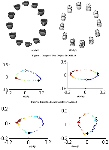
The embedded manifolds before aligned are shown in Figure 2, and the embedded manifolds after aligned are shown in Figure 3. The matching points for aligning the manifold of different image sequences are marked as large dots by different colors(red, white, black). We can see that our algorithms can align the embedded manifolds properly with the knowledge extracted from the matching points and the relationship among points of each image sequence.

[image:5.595.118.481.167.667.2]

(a)obj1 (b)obj2

Figure 1. Images of Two Objects in COIL20

(a)obj1 (b)obj2

Figure 2 Embedded Manifolds Before Aligned

(a)obj1 (b)obj2

Figure 3. Embedded Manifolds After Aligned

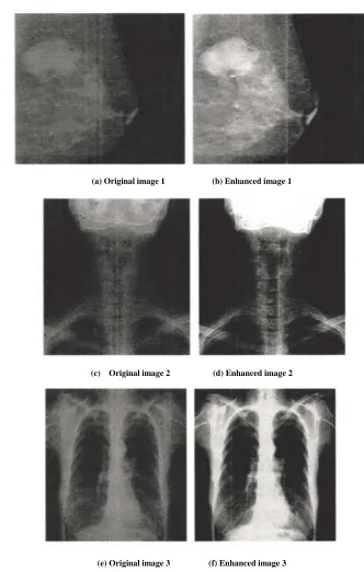
(a) Original image 1 (b) Enhanced image 1

(c) Original image 2 (d) Enhanced image 2

[image:6.595.123.455.98.620.2]

(e) Original image 3 (f) Enhanced image 3

Figure 4. Enhancement contrast of DR image

CONCLUSION

Acknowledgments

This paper is supported by Scientific Research Fund of Hunan Provincial Education Department (Grant no.12B023).

REFERENCES

[1] J.Ham; D.Lee; L.Saul, Proc. 10th Int’l Workshop Artificial Intelligence and Statistics, page 120-127, 2005. [2] A.P.Shon; K.Grochow; A.Hertzmann; R.Rao, In Proc. NIPS, page 1233–1240, 2006.

[3] S.Lafon; Y.Keller; R.R.Coifman, IEEE PAMI, 28(11): 1784-1797, 2006. [4] Z.Zhang; H.Zha, SIAM J. Sci. Comput. 26 (1): 313–338, 2004.

[5] X.Bai; H.Yu; E.R , Proc. Int’l Conf. Pattern Recognition, page 398-401, 2004. [6] M.Gori; M.Maggini; L.Sarti, IEEE PAMI, 27(7): 1100-1111, 2005.

[7] Y.Keselman; A.Shokoufandeh; M.F.Demirci; S.J. Dickinson, Proc. Conf. Computer Vision and Pattern Recognition, page 850-857, 2003.

[8] J.Black; M.Gargesha; K.Kahol; P.Kuchi; S.Panchanathan, ITCOM, Internet Multimedia Systems II, Boston, July 2002.