Bootstrap Tests Based on Goodness of Fit Measures for Nonnested Hypotheses in Regression Models

Munich Personal RePEc Archive

Bootstrap Tests Based on

Goodness-of-Fit Measures for Nonnested

Hypotheses in Regression Models

Jeong, Jinook

Yonsei University

April 2006

Online at

https://mpra.ub.uni-muenchen.de/9789/

Bootstrap Tests Based on Goodness-of-Fit Measures for Nonnested

Hypotheses in Regression Models

by

Jinook Jeong Department of Economics

Yonsei University

February 2007

Abstract

This paper utilizes the bootstrap to construct tests using the measures for goodness-of-fit for nonnested regression models. The bootstrap enables us to compute the statistical significance of the differences in the measures and to formally test on nonnested regression models. The bootstrap tests that this paper proposes are expected to show better finite sample properties since they do not have accumulated errors in the computation process. Moreover, the bootstrap tests remove the possibility of inconsistent test results that the previous tests suffer from. Because the bootstrap tests only evaluate if a model has a significantly higher explanatory power than the other model, there is no possibility for inconsistent results. This study presents Monte Carlo simulation results to compare the finite sample properties of the proposed tests with the previous tests such as Cox test and J-test.

Keywords: nonnested regression models, bootstrap, goodness-of-fit measures

JEL Classification: C12, C14, C15

Acknowledgements: I am grateful for the helpful comments from Tae-Hwan Kim, Tae-Kyu Park and the participants of Yonsei Economic Research Institute seminar. I am also grateful for the excellent research assistance by So Yeon Park, Sung Sam Chung and Byunguk Kang. This work was supported by Korea Research Foundation Grant (KRF-2002-041-B00055).

Correspondences: Professor Jinook Jeong Department of Economics Yonsei University

Seoul, Korea 120-749

1. Introduction

When a researcher chooses from nonnested regression models, it is difficult to apply the

usual F-test because there do not exist testable common restrictions.1 There have been

proposed several tests for nonnested hypotheses in the literature. Cox test has been originally

proposed by Cox (1961, 1962) and further developed by Pesaran (1974) and Pesaran and

Deaton (1978) for nonnested regression models. Cox test is a likelihood ratio test comparing

the likelihood under model 1 (H1) to the one under model 2 (H2). Cox test has some

shortcomings. It is computationally burdensome and is not robust to distributional assumption.

Also, the consistency in its test result is not guaranteed: it may favor H1 over H2, and at the same

time favor H2 over H1. Third, as the test is based on an asymptotic distribution, the power in

finite samples is questionable.

Davidson and MacKinnon (1981) suggest J-test for nonnested regression models. J-test

is a two-step test based on ‘artificial nesting.’ Though J-test is easier and more practical than

Cox test, it still has the problem of inconsistent test results as Cox test. Also, as it is based on an

asymptotic distribution, the small sample performance of J-test is not satisfactory. Godfrey

(1998), Fan and Li (1995), and Davidson and MacKinnon (2002) apply bootstrap procedures

for J-test and succeed to improve its power in finite samples. However, the possibility of

inconsistent test results still remains.

Another approach to nonnested models is the tests based on ‘encompassing principle.’

All the above tests assume that the true conditional distribution of the data is either H1 or H2.

However, in practice, there always exists the third possibility. Mizon and Richard (1986)

among others criticize the assumption and propose Encompassing test which include J-test as a

special case.

There are many other test procedures for nonnested regression model in the literature.

1

However, all the previous tests have two common problems. First, the possibility of

inconsistent test results prevails. Second, the test power in finite samples is not satisfactory.

The low power can be explained in two ways. One, most tests use asymptotic distributions

which is not accurate enough in small samples. Two, as most previous tests involve complex

computation, they may suffer from some distortion of information in the process of

computation. For example, J-test uses the predicted values from the first stage regression in the

second stage. As a result, the estimation error in the first stage regression is carried over to the

second stage and reduces the accuracy of the second stage results as Pagan (1984, 1986) points

out.

This paper suggests a simple new test procedure for nonnested regression models.

When we consider two competing regression models, the first comparison we usually do is the

coefficient of determination (R2) of the models. R2 is probably the simplest and most intuitive

measure for the fit of a regression model, although there exist a number of alternative measures

such as adjusted R2 (R ), Akaike Information Criterion (AIC), Bayesian Information Criterion 2

(BIC), Predicted Residual Sum of Squares (PRESS), and Hocking’s Sp, among others.

However, it has not been possible to construct a test with such measures for model selection,

since none of the exact distributions of the measures or of the difference (or ratio) of the

measures is known. Comparison of the goodness-of-fit measures is limited only to eyeball

inspection and intuitive benchmarking.

This paper utilizes a computation-oriented nonparametric method, the bootstrap, to

construct tests using the goodness-of-fit measures for nonnested regression models. The

bootstrap enables us to compute the statistical significance of the differences in those measures

and to formally test about nonnested regression models. It is not new to apply bootstrap

procedures for nonnested regression models. As mentioned above, bootstrap has been applied

been maximized as J-test has the problem of accumulated errors from its two-step procedure.

Bootstrap tests that this paper proposes are expected to show better finite sample properties

since they do not have such accumulated errors in the computation process. Moreover, the

bootstrap tests using goodness-of-fit measures have another important advantage: there is no

possibility of inconsistent test results. Because the bootstrap tests only evaluate if a model has

a significantly higher explanatory power than the other model, inconsistent results cannot

happen. We present Monte Carlo simulation results to compare the finite sample properties of

the proposed tests with the previous tests such as Cox test and J-test.

2. Model

Consider the following two regression models.

H1: y = Xβ + u (1)

H2: y = Zγ + v (2)

where y is the (n×1) vector of the dependent variable, X and Z are (n×k1) and (n×k2) matrices of

regressors, and u and v are (n×1) vectors of errors. We assume that E(u) = E(v) = 0 and var(u)

=σ₁2I and var(v) =σ2₂I. We also assume the two alternative sets of regressors, X and Z, may

have some common variables, but neither is a subset of the other. The problem here is to decide

which is a better model.

Cox (1961, 1962) developed a variant of likelihood ratio test for nonnested hypotheses.

Pesaran (1974), Pesaran and Deaton (1978), and McAleer (1984) have derived various versions

of Cox test for the regression cases. For our hypotheses (1) and (2), the Cox statistic for testing

that H1 is correct and H2 is not is,

⎥ ⎦ ⎤ ⎢ ⎣ ⎡

= ₂

ZX 2 Z 12

s s log 2 n

c (3)

The test statistic of Cox test is as follows. 4 ZX Z X Z 2 X 12 12 12 s ) ˆ X M M M ' X ' ˆ ( s c ) c ( SE c β β

= (4)

where 'M_X =I−X(X'X)−1X . Cox has shown that the test statistic in (4) is asymptotically

distributed as a standard normal variable under H1. A significantly larger value of the statistic

from zero is evidence against H1.

The J test proposed by Davidson and MacKinnon (1981) is a linearized version of the

Cox test. It uses the following ‘artificially nested’ model.

y = (1−λ)Xβ + λZγ + e (5)

In this model, if the hypothesis H1 is true, then λ = 0. The problem is that λ is not identified in

the estimation of equation (5). Davidson and MacKinnon (1981) suggest a two-step procedure:

γ is estimated by least squares from equation (2), and the estimator, γˆ, is replaced for the

unknown γ in equation (5) to separately estimate λ. Thus in the second stage, the following

equation is estimated by least squares.

y = (1−λ)Xβ + λ(Zγˆ) + e (6)

As Pesaran (1982) shows, if H1 is true, the test statistic becomes:

) ˆ Z M ' Z ' ˆ ( s y M ' Z ' ˆ J X 2 1 X 1 γ γ γ

= (7)

where s is the estimated error variance of regression in (6). J₁2 1 is asymptotically distributed as

a standard normal variable. A large value of J1 is evidence against H1.

Similarly, the test statistic J2 can be derived for a test of H2 against H1 in the following

model.

) ˆ X M ' X ' ˆ ( s y M ' X ' ˆ J Z 2 2 Z 2 β β β

= (9)

where s is the estimated error variance of regression in (8). As discussed in the introduction, 2₂

the result of the J1 test and the J2 test may not be consistent. It is possible that the tests reject

both, neither, or either one of the hypotheses H1 and H2.

There are a number of alternative versions of the J tests by using different estimates of γ

in equation (6) and β in equation (8). The alternative tests are summarized in Davidson and

MacKinnon (2004).

3. Bootstrapping the difference in Goodness-of-Fit Measures

First, the coefficient of determination, R2, of a regression model y = Xβ + u is defined as

follows.2 ) y y ( )' y y ( uˆ ' uˆ 1 R2 − − − = (10)

where uˆ=y−Xβˆ and βˆ is the least squares estimator of β. The distribution of R2 for normally

distributed errors has been derived by Cramer (1987) among others. Assuming u ~ N(0, σ2I),

the dimension of y is (n×1), the dimension of X is (n×k), and the first column in X is a vector of

ones, the density function of R2, with argument r, is:

∑

= −λ ,

2 1 k p= − ,

2 1 n

q= − , and B(·) is the beta function.

For two competing regression models with normally distributed errors, e.g. (1) y = Xβ +

u and (2) y = Zγ + v, Schmidt (1973) suggests a numerical method for calculating

2

) R R (

P 2

Zy 2

Xy> when model (1) is true. Ebbeler (1975) extends Schmidt’s work to the adjusted

R2 (i.e. R ) comparison. Though their works allow us to estimate the probability of correct 2

model selections based on R2 (or R ) under normality assumption, it is still an open question 2

how to compute the statistical significance of an observed difference in two R2’s.

The advantages of bootstrapping the difference in R2’s (and in the other measures of

goodness-of-fit) are as follows. First, it allows us to compute the significance of an observed

difference in two R2’s using the empirical (bootstrap) distribution of the difference.

Accordingly, one can perform a test on alternative models with the computed significance level.

Second, bootstrap method is robust to the distributional assumption. Even though the

distribution of error terms is not normal, bootstrap can still compute the statistical significance

of the observed difference in R2’s.

It should be noted that the R2’s are not pivotal, and the standard bootstrap confidence

interval may not work well. In this paper, two alternative bootstrap procedures are employed.

First, the standard simple bootstrap confidence interval is applied to ‘transformed’ R2’s to

overcome the range-restrictiveness.3 Second, a double bootstrapped confidence interval is

employed for the transformed R2’s (and other goodness-of-fit measures). The double bootstrap

procedure is: (a) draw the bootstrap sample, (b) estimate the standard error of the statistic of

interest θˆ , sB, by a ‘nested’ bootstrap procedure, (c) using the formula

B 0

s ˆ

t = θ−θ , a

‘prepivoted’ root t is constructed, and (d) determine the critical values for the test from the

‘outer’ bootstrap empirical distribution of the root t by repeating (a) through (c).4

Similar standard and double bootstrap procedures are applied to the alternative

3

The

2 2

R 1

R

− transfrormation has been used. Actually, the results with the original form of R

2

and the results with

the transformed R2 are not much different. The detailed results are available from the author upon request.

4

measures for goodness-of-fit: R , AIC, BIC, PRESS, and Hocking’s S2 p.5 The definitions of

the measures are as follows.6

) R 1 ( k n 1 n 1

R2 − 2

− − − ≡ (12) n k 2 n uˆ ' uˆ log

AIC ⎟+

⎠ ⎞ ⎜ ⎝ ⎛

≡ (13)

n ) n (log k n uˆ ' uˆ log

BIC ⎟+

⎠ ⎞ ⎜ ⎝ ⎛

≡ (14)

* *

u ' u

PRESS≡ (15)

) 1 k n )( k n ( uˆ ' uˆ S_p − − −

≡ (16)

where i i * i h 1 uˆ u −

≡ , and hi is the ith diagonal element of X(X'X)−1X. The results are compared

along with the Cox test and J test in the nest section.

4. Finite Sample Performance of Alternative Tests for Nonnested Regression Models

To compare the finite sample performances of the alternative tests for nonnested

regression models, we adopt the Monte Carlo design of Godfrey (1998) for equation (1) and (2).

The elements xij of X are N(0,22) variables that are independent over i and j, i = 1, 2, …, n and j

= 1, 2, …, k1. The elements zij of Z are generated as follows.

ij ij

ij x e

z =α + j = 1, 2, …, min(k1, k2) (17)

ij

ij e

z = j = k1+1, k1+2, …, k2 (if k1 < k2) (18)

We assume that eij are independent random picks from N(0,22), and that the error terms of (1)

and (2), ui and vi , are independent random picks from normal distributions with zero means and

5

Mallows’ Cp is another widely-used measure for goodness-of-fit. I use Hocking’s Sp rather than Mallows’ Cp for

two reasons. First, Mallows’ Cp requires the knowledge of the error variance. Second, it has been shown by Kinal

and Lahiri (1984) that the stochastic version of Mallows’ Cp is identical to Hocking’s Sp.

6

variances of 2 u

σ and 2 v

σ , respectively.7 Without loss of generality, we set every element of β

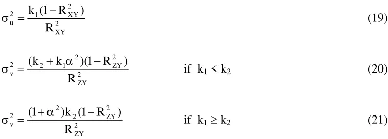
and γ is one. To maintain a constant R2 in a simulation, σ2_u and σ2_v are set as follows.8

2 XY 2 XY 1 2 u R ) R 1 ( k − = σ (19) 2 ZY 2 ZY 2 1 2 2 v R ) R 1 )( k k

( + α −

=

σ if k1 < k2 (20)

2 ZY 2 ZY 2 2 2 v R ) R 1 ( k ) 1

( +α −

=

σ if k1≥ k2 (21)

The value of α is determined by the correlation between xij and zij. With the correlation

coefficient ρ between xij and zij,

2

1−ρ

ρ =

α .

Table 1 and Table 2 present the performances of alternative tests when the numbers of

regressors (k1 and k2) are symmetric. The tests compared in the simulations are: Cox test

(‘Cox’ in the Tables), J-test (‘J’ in the Tables), R2, R , AIC, BIC, PRESS, and S2 p. All the

goodness-of-fit measures (R2, R , AIC, BIC, PRESS, and S2 p) are bootstrapped through two

alternative procedures, as explained in section 3: standard bootstrap (‘SB’ in the Tables) and

double bootstrap (‘DB’ in the Tables). Thus, we compare all 14 alternative test procedures as in

Tables 1 and 2.

For these 14 alternative tests, Tables 1 and 2 show the rejection rates of H1: y = Xβ + u

when H2: y = Zγ + v is the true model. The rejection rates are reported for various values of ρ,

the correlation coefficients between xij and zij. When ρ is low, it should be easy for any test to

distinguish the true model (H2 here) from the wrong model (H1). As ρ becomes higher, it must

be more difficult for any test to reject the wrong model against the true model. When ρ=1, both

7

the models become identical and the test should reject the wrong model only for the nominal

size. In the simulations, because α is not defined when ρ=1, the rejection rates of H1 when

ρ=0.9999 instead are computed. Thus, the rejection rates reported in the far-right column of

ρ=0.9999 represent the ‘empirical sizes’ of the tests. To capture the finite sample performances

of the alternative tests, four different sample sizes are employed in the Monte Carlo simulation:

20, 50, 100, and 200. The frequency of resampling in the process of bootstrap is set to 500. The

simulation is done 1000 times.9

Table 1 shows the rejection rates of the 14 alternative tests when each model (H1 and

H2) has two regressors, i.e. k1=2 and k2=2. It is clear from Table 1 that the bootstrap tests

outperform Cox test and J-test. First of all, the empirical sizes of the bootstrap tests are more

accurate than Cox test or J-test. For all the sample sizes, the empirical sizes of Cox test and

J-test are much smaller than the nominal size of 0.05. For example, when the sample size is 50,

the empirical size of Cox test is 0.002 and the empirical size of J-test is 0.001. The empirical

sizes of bootstrap tests are much closer to the nominal level. For the same case of sample size

of 50, the empirical size of standard bootstrap test using R2 is 0.053. All the other measures

show similar empirical sizes ranging from 0.051 to 0.087 for n = 50. Regardless of the error

distribution or the sample size, the bootstrap tests show reasonably better size than Cox test or

J-test.10

It is also obvious from Table 1 that the bootstrap tests have higher power than Cox test

or J-test. For the whole range (0.00 to 0.95) of ρ, the standard bootstrap test and double

bootstrap test produce consistently higher empirical power that Cox test or J-test. For example,

let us look at the case when the sample size is 100 and ρ equals 0.75. The empirical power of

distributions.

8

If β or γ is not a vector of ones, these expressions would become a bit more complex.

9

For the double bootstrap procedures, to reduce the computational burden, the nested bootstrap repetition is reduced to 100 times, the outer bootstrap repetition is reduced to 200 times, and the simulation is done 300 times.

10

Cox test is 0.953 and the empirical power of J-test is 0.951 while the empirical powers of the

bootstrap tests are all 1.000. For all the sample sizes and all the values of ρ, the bootstrap tests

show better power than Cox test or J-test.

Table 2 repeats the same findings for the case of four regressors in each model (k1=4

and k2=4). Although the performances of the four tests are a bit worse than Table 1 (k1=2 and

k2=2 case) due to the reduction in the degrees of freedom, the simulation results basically tell us

that the bootstrap tests have more accurate size and higher power. The reason why Cox test and

J-test under-reject the null hypothesis should be related to the problems explained in section 2.

Especially, the inconsistency in the test results of Cox test and J-test may have weakened the

performance of the tests. It is possible for the two tests show inconsistent results, because Cox

test and J-test evaluate the hypothesis twice: once test H1 against H2, and then test H2 against H1.

Table 3 presents how frequently Cox test and J-test produce inconsistent test results. As seen in

the Table, in all the cases considered in the simulation, Cox test and J-test show considerable

rates of the inconsistent results. These inconsistent results have lowered the power of Cox test

and J-test. Besides, as explained in section 2, the complexity of computation in Cox test and the

two-step estimation process in J-test may have created distortions.

It has been argued that the finite sample properties of J-test may become problematic

when the two competing models have asymmetric numbers of regressors. Davidson and

MacKinnon (2002, 2004) give a good summary of the asymmetric regressor problem in J-test.11

Unfortunately, because R2 is not robust to the number of regressors, it is also reasonable to

expect that the performance of any test using R2 would not be ideal for asymmetric regressor

cases. However, as the other measures of goodness-of-fit are robust to the number of regressors,

their performances may not be affected by the asymmetry of the models. To see the effects of

asymmetric regressors, Tables 4 – 5 report the rejection rates of the fourteen tests in various

results are available from the author upon request.

11

combinations of asymmetric regressor cases.

Table 4 shows the rejection rates of the alternative tests when the X-model (H1) has 2

regressors and the Z-model (H2) has 4 regressors, that is, k1=2 and k2=4. Since the true data

generation process in the simulation is Z-model, the situation is that the true model has more

regressors than the wrong model. As expected, the finite sample performances of the bootstrap

tests using R2’s, as well as Cox test or J-test, are far from perfect. All the four tests over-reject

the true model.12 The magnitude of such over-rejection is highest with standard bootstrap test

using R2, and lowest with J-test. Overall, however, none of the four tests is acceptable in terms

of empirical size.

It is not surprising that the tests using R2 do not perform well. It is well known that R2

does not provide any penalty for adding irrelevant regressors. To remedy the limitation of R2,

the alternative measures have been proposed such as R , AIC, BIC, PRESS, and S2 p. The

bootstrap tests using these measures show much better performance. For example, when n = 20,

the empirical size of standard bootstrap test using R is 0.059 and the empirical size of double 2

bootstrap test using R is 0.053 respectively, which are pretty close to the nominal size of 2

0.050. The tests using AIC, BIC, PRESS or Sp somewhat under-rejects the true model, but their

rejection rates are much closer to the nominal size than Cox test, J-test, and the bootstrap tests

using R2.

Tables 5 shows the effects of regressor asymmetry in the opposite way: the X-model

(H1) has more regressors than the Z-model. Thus, the wrong model now has more regressors

than the true model. Table 5 presents the rejection rates of X-model for the alternative tests

when k1=4 and k2=2. In this case, J-test shows the most accurate size, and all the other tests

show the tendency of under-rejection when the null hypothesis is true. In terms of power,

however, J-test does not show as high power as the bootstrap tests using R2, R , AIC, BIC, 2

12

PRESS or Sp except when n = 20. One interesting phenomenon about BIC is that the empirical

size of bootstrapped BIC test tends to increase as the sample size grows. For example, the

empirical size of the standard bootstrap test using BIC is 0.008 when n = 20, 0.214 when n = 50,

0.432 when n = 100, and as high as 0.600 when n = 200. The empirical sizes of double

bootstrap test using BIC have weaker tendency of escalating but still increases as the sample

size becomes larger: 0.000 when n = 20, 0.037 when n = 50, 0.220 when n = 100, and as high as

0.400 when n = 200. This is probably due to the definition of BIC. As shown in (14), BIC

penalizes the inclusion of more explanatory variables with a factor of log(n). Due to such

definition, the penalty for including more explanatory variables depends on the number of

samples (n). In short, BIC gives too much penalty for inclusion of new explanatory variables,

and the over-penalization escalates with the sample size.

6. Conclusion

This paper suggests a simple new test procedure for nonnested regression models. It

utilizes a computation-oriented nonparametric method, the bootstrap, to construct a test using

various measures for goodness-of-fit such as R2 , R , AIC, BIC, PRESS, and S2 p for nonnested

regression models. The bootstrap enables us to compute the statistical significance of the

differences in those measures and to formally test to choose the best model among nonnested

regression models. The bootstrap tests that this paper proposes have an obvious strength over

the existing ones: they never show inconsistent test results. Because the bootstrap tests only

evaluate if a model has a significantly higher explanatory power than the other model, there is

no possibility for inconsistent results.

The Monte Carlo simulation results to compare the finite sample properties of the

proposed tests with the previous tests such as Cox test and J-test show that the proposed

previous tests when the number of regressors are symmetric. In the cases of asymmetric

regressor cases, however, the finite sample performances of the suggested bootstrap tests show

some mixed results. Overall, the bootstrap tests using R show the best finite sample 2

References

Cox, D.R. (1961), "Test of Seperate Families of Hypotheses," Proceedings of the Fourth

Berkeley Symposium on Mathematical Statistics and Probability 1, pp.105-123

Cox, D.R. (1962), "Further Results on Tests of Separate Families of Hypotheses," Journal of the Royal Statistical Society 24, pp.406-24

Cramer, J.S. (1987), “Mean and Variance of R2 in Small and Moderate Samples,” Journal of

Econometrics 35, pp.253-266

Davidson, R. and J.G. MacKinnon (1981), "Several Tests for Model Specification in the Presence of Alternative Hypotheses," Econometrica 49 , pp.781-793

Davidson, R. and J.G. MacKinnon (2002), "Bootstrap J Tests of Non-nested Linear Regression Models," Journal of Econometrics 109 , pp.167-193

Davidson, R. and J.G. MacKinnon (2004), Econometric Theory and Methods, Oxford University Press, New York.

Ebbeler, D.H. (1975), “On the Probability of Correct Model Selection Using the Maximum R 2 Choice Criterion,” International Economic Review 16, pp.516-520.

Fan, Y. and Q. Li (1995), "Bootstrapping J-type Tests for Non-nested Regrssion Models,"

Economics Letters 48 , pp.107-112

Godfrey, L.G. (1998), "Tests of Non-nested Regression models : Some Results on Small Sample Behaviour and the Bootstrap," Journal of Econometrics 84 , pp.59-74

Jeong, J. and S. Chung (2001), "Bootstrap Tests for Autocorrelation," Computational Statistics

and Data Analysis 38, pp.49-69.

Jeong, J. and G.S. Maddala (1993), "A Perspective on Application of Bootstrap Methods in Econometrics," Handbook of Statistics, Volume 11: Econometrics, North-Holland, (ed) by G.S. Maddala, C.R. Rao, and H.D. Vinod, pp.573-610.

Kinal, T. and K. Lahiri (1984), “A Note on ‘Selection of Regressors,’” International Economic

Review 25, pp.625-629.

McAleer, M. (1984), "Specification Tests for Separate Models: A Survey," in M.L. King and D.E.A. Giles (eds), Specification Analysis in the Linear Model: Essays in Honor of Donald Cochrane

Mizon, G.E. and J.F. Richard (1986), "The Encompassing Principle and its Application to Testing Non-nested Hypotheses," Econometrica 54 , pp.657-678

Pagan, A. (1984), "Econometric issues in the analysis of regressions with generated regressors," International Economic Review 25, pp.221-247.

Economic Studies 53, pp.517-538

Pesaran, M.H. (1974), "On the General Problem of Model Selection," Review of Economic Studies 41 , pp.153-171

Pesaran, M.H. and A.S. Deaton (1978), "Testing Non-nested Nonlinear Regression Models,"

Econometrica 46 , pp.677-694

Pesaran, M.H. (1982), "Comparison of Local Power of Alternative Tests of Nonnested Regression Models," Econometrica 50, pp.1287-1306

Schmidt, P. (1973), “Calculating the Power of the Minimum Standard Error Choice Criterion,”

<Table 1> Rejection Rates of H1: y = Xβ + u (k1=2, k2=2) True Model: H2, True Rzy2 = 0.9, Nominal Size = 0.05.

ρ 0.00 0.30 0.60 0.70 0.75 0.80 0.85 0.90 0.95 0.9999

n=20

Cox 0.907 0.912 0.930 0.920 0.926 0.913 0.923 0.931 0.924 0.005 J 0.919 0.912 0.922 0.925 0.918 0.908 0.928 0.936 0.918 0.008 SB (R2) 1 1 1 1 1 1 0.999 0.999 0.959 0.065 DB (R2) 1 1 1 1 1 1 1 1 0.970 0.067 SB ( 2

R ) 1 1 1 1 1 1 0.999 0.999 0.959 0.065 DB ( 2

R ) 1 1 1 1 1 1 1 1 0.970 0.063

SB (AIC) 1 1 1 1 1 1 0.999 0.999 0.959 0.065 DB (AIC) 1 1 1 1 1 1 1 1 0.970 0.060 SB (BIC) 1 1 1 1 1 1 0.999 0.999 0.959 0.065 DB (BIC) 1 1 1 1 1 1 1 1 0.970 0.060 SB (PRESS) 1 1 1 1 1 1 1 0.999 0.955 0.068 DB (PRESS) 1 1 1 1 1 1 1 1 0.967 0.073 SB (Sp) 1 1 1 1 1 1 0.999 0.999 0.959 0.065

DB (Sp) 1 1 1 1 1 1 1 1 0.967 0.067

n=50

Cox 0.921 0.946 0.929 0.937 0.946 0.945 0.937 0.944 0.939 0.002 J 0.932 0.940 0.923 0.933 0.950 0.940 0.934 0.952 0.949 0.001

SB (R2) 1 1 1 1 1 1 1 1 1 0.053

DB (R2) 1 1 1 1 1 1 1 1 1 0.083

SB ( 2

R ) 1 1 1 1 1 1 1 1 1 0.053

DB ( 2

R ) 1 1 1 1 1 1 1 1 1 0.083

SB (AIC) 1 1 1 1 1 1 1 1 1 0.053

DB (AIC) 1 1 1 1 1 1 1 1 1 0.073

SB (BIC) 1 1 1 1 1 1 1 1 1 0.053

DB (BIC) 1 1 1 1 1 1 1 1 1 0.073

SB (PRESS) 1 1 1 1 1 1 1 1 1 0.051

DB (PRESS) 1 1 1 1 1 1 1 1 1 0.087

SB (Sp) 1 1 1 1 1 1 1 1 1 0.053

DB (Sp) 1 1 1 1 1 1 1 1 1 0.087

n=100

Cox 0.923 0.940 0.943 0.942 0.953 0.950 0.946 0.947 0.937 0.006 J 0.936 0.942 0.950 0.943 0.951 0.948 0.948 0.950 0.942 0.006

SB (R2) 1 1 1 1 1 1 1 1 1 0.065

DB (R2) 1 1 1 1 1 1 1 1 1 0.067

SB ( 2

R ) 1 1 1 1 1 1 1 1 1 0.065

DB ( 2

R ) 1 1 1 1 1 1 1 1 1 0.067

SB (AIC) 1 1 1 1 1 1 1 1 1 0.065

DB (AIC) 1 1 1 1 1 1 1 1 1 0.060

SB (BIC) 1 1 1 1 1 1 1 1 1 0.065

DB (BIC) 1 1 1 1 1 1 1 1 1 0.060

SB (PRESS) 1 1 1 1 1 1 1 1 1 0.065

DB (PRESS) 1 1 1 1 1 1 1 1 1 0.070

SB (Sp) 1 1 1 1 1 1 1 1 1 0.065

n=200

Cox 0.935 0.946 0.942 0.958 0.945 0.939 0.948 0.954 0.954 0.011 J 0.942 0.948 0.940 0.951 0.945 0.941 0.945 0.954 0.953 0.010

SB (R2) 1 1 1 1 1 1 1 1 1 0.079

DB (R2) 1 1 1 1 1 1 1 1 1 0.043

SB (R2) 1 1 1 1 1 1 1 1 1 0.079

DB (R2) 1 1 1 1 1 1 1 1 1 0.043

SB (AIC) 1 1 1 1 1 1 1 1 1 0.079

DB (AIC) 1 1 1 1 1 1 1 1 1 0.040

SB (BIC) 1 1 1 1 1 1 1 1 1 0.079

DB (BIC) 1 1 1 1 1 1 1 1 1 0.040

SB (PRESS) 1 1 1 1 1 1 1 1 1 0.079

DB (PRESS) 1 1 1 1 1 1 1 1 1 0.050

SB (Sp) 1 1 1 1 1 1 1 1 1 0.079

<Table 2> Rejection Rates of H1: y = Xβ + u (k1=4, k2=4) True Model: H2, True Rzy2 = 0.9, Nominal Size = 0.05.

ρ 0.00 0.30 0.60 0.70 0.75 0.80 0.85 0.90 0.95 0.9999

n=20

Cox 0.900 0.891 0.905 0.910 0.912 0.902 0.898 0.889 0.885 0.005 J 0.908 0.914 0.920 0.924 0.933 0.915 0.907 0.909 0.912 0.001 SB (R2) 1 1 1 1 1 0.999 0.995 0.991 0.928 0.052 DB (R2) 1 1 1 1 1 0.997 0.990 0.993 0.963 0.063 SB ( 2

R ) 1 1 1 1 1 0.999 0.995 0.991 0.928 0.052 DB ( 2

R ) 1 1 1 1 1 0.997 0.990 0.993 0.963 0.063 SB (AIC) 1 1 1 1 1 0.999 0.995 0.991 0.928 0.052 DB (AIC) 1 1 1 1 1 0.997 0.990 0.993 0.963 0.050 SB (BIC) 1 1 1 1 1 0.999 0.995 0.991 0.928 0.052 DB (BIC) 1 1 1 1 1 0.997 0.990 0.993 0.963 0.050 SB (PRESS) 1 1 1 1 1 0.999 0.995 0.990 0.924 0.039 DB (PRESS) 1 1 1 1 1 0.997 0.990 0.983 0.950 0.057 SB (Sp) 1 1 1 1 1 0.999 0.995 0.991 0.928 0.052

DB (Sp) 1 1 1 1 1 0.997 0.990 0.993 0.957 0.063

n=50

Cox 0.923 0.929 0.944 0.947 0.937 0.930 0.945 0.924 0.933 0.005 J 0.925 0.934 0.945 0.952 0.939 0.935 0.947 0.934 0.941 0.005

SB (R2) 1 1 1 1 1 1 1 1 1 0.076

DB (R2) 1 1 1 1 1 1 1 1 1 0.083

SB ( 2

R ) 1 1 1 1 1 1 1 1 1 0.076

DB ( 2

R ) 1 1 1 1 1 1 1 1 1 0.083

SB (AIC) 1 1 1 1 1 1 1 1 1 0.076

DB (AIC) 1 1 1 1 1 1 1 1 1 0.080

SB (BIC) 1 1 1 1 1 1 1 1 1 0.076

DB (BIC) 1 1 1 1 1 1 1 1 1 0.080

SB (PRESS) 1 1 1 1 1 1 1 1 1 0.070

DB (PRESS) 1 1 1 1 1 1 1 1 1 0.087

SB (Sp) 1 1 1 1 1 1 1 1 1 0.076

DB (Sp) 1 1 1 1 1 1 1 1 1 0.087

n=100

Cox 0.919 0.945 0.937 0.940 0.947 0.936 0.943 0.938 0.954 0.002 J 0.922 0.948 0.938 0.940 0.951 0.933 0.942 0.946 0.959 0.002

SB (R2) 1 1 1 1 1 1 1 1 1 0.057

DB (R2) 1 1 1 1 1 1 1 1 1 0.063

SB ( 2

R ) 1 1 1 1 1 1 1 1 1 0.057

DB ( 2

R ) 1 1 1 1 1 1 1 1 1 0.063

SB (AIC) 1 1 1 1 1 1 1 1 1 0.057

DB (AIC) 1 1 1 1 1 1 1 1 1 0.060

SB (BIC) 1 1 1 1 1 1 1 1 1 0.057

DB (BIC) 1 1 1 1 1 1 1 1 1 0.060

SB (PRESS) 1 1 1 1 1 1 1 1 1 0.057

DB (PRESS) 1 1 1 1 1 1 1 1 1 0.073

SB (Sp) 1 1 1 1 1 1 1 1 1 0.057

n=200

Cox 0.933 0.941 0.946 0.949 0.947 0.945 0.944 0.946 0.955 0.008 J 0.937 0.944 0.945 0.951 0.946 0.950 0.945 0.947 0.955 0.008

SB (R2) 1 1 1 1 1 1 1 1 1 0.060

DB (R2) 1 1 1 1 1 1 1 1 1 0.063

SB ( 2

R ) 1 1 1 1 1 1 1 1 1 0.060

DB ( 2

R ) 1 1 1 1 1 1 1 1 1 0.063

SB (AIC) 1 1 1 1 1 1 1 1 1 0.060

DB (AIC) 1 1 1 1 1 1 1 1 1 0.060

SB (BIC) 1 1 1 1 1 1 1 1 1 0.060

DB (BIC) 1 1 1 1 1 1 1 1 1 0.060

SB (PRESS) 1 1 1 1 1 1 1 1 1 0.057

DB (PRESS) 1 1 1 1 1 1 1 1 1 0.067

SB (Sp) 1 1 1 1 1 1 1 1 1 0.060

<Table 3> Rates of Inconsistent Test Results

Error Distribution: Normal (0,1), k1=2, k2=2

　 0.00 0.30 0.60 0.70 0.75 0.80 0.85 0.90 0.95 0.9999

n=20 Cox 0.063 0.091 0.054 0.070 0.073 0.064 0.077 0.066 0.102 0.993 J 0.071 0.089 0.064 0.081 0.075 0.073 0.084 0.065 0.085 0.992

n=50 Cox 0.082 0.071 0.058 0.056 0.062 0.056 0.070 0.063 0.040 0.995 J 0.065 0.072 0.059 0.057 0.067 0.050 0.070 0.059 0.039 0.996

n=100 Cox 0.063 0.050 0.050 0.056 0.056 0.055 0.051 0.064 0.056 0.990 J 0.054 0.049 0.054 0.059 0.053 0.056 0.050 0.065 0.060 0.989

n=200 Cox 0.069 0.059 0.051 0.068 0.057 0.050 0.047 0.046 0.047 0.990 J 0.057 0.054 0.049 0.066 0.057 0.049 0.048 0.045 0.050 0.989

Error Distribution: Uniform (0,1), k1=2, k2=2

　 0.00 0.30 0.60 0.70 0.75 0.80 0.85 0.90 0.95 0.9999

n=20 Cox 0.101 0.082 0.063 0.063 0.074 0.060 0.081 0.073 0.086 0.995 J 0.091 0.067 0.068 0.069 0.077 0.066 0.084 0.067 0.085 0.993

n=50 Cox 0.069 0.049 0.059 0.055 0.064 0.053 0.057 0.046 0.053 0.992 J 0.057 0.053 0.064 0.057 0.065 0.058 0.051 0.049 0.052 0.992

n=100 Cox 0.072 0.070 0.049 0.059 0.055 0.058 0.055 0.058 0.051 0.991 J 0.067 0.066 0.053 0.055 0.057 0.059 0.053 0.060 0.055 0.991

n=200 Cox 0.075 0.061 0.052 0.056 0.051 0.059 0.062 0.062 0.046 0.983 J 0.061 0.065 0.054 0.048 0.056 0.061 0.060 0.059 0.046 0.983

Error Distribution: Normal (0,1), k1=4, k2=4

　 0.00 0.30 0.60 0.70 0.75 0.80 0.85 0.90 0.95 0.9999

n=20 Cox 0.112 0.101 0.099 0.095 0.101 0.094 0.098 0.118 0.098 0.992 J 0.099 0.084 0.077 0.086 0.08 0.074 0.082 0.089 0.073 0.991

n=50 Cox 0.074 0.063 0.068 0.061 0.064 0.060 0.074 0.071 0.066 0.988 J 0.065 0.059 0.069 0.060 0.054 0.059 0.070 0.066 0.060 0.988

n=100 Cox 0.067 0.053 0.069 0.068 0.048 0.053 0.066 0.066 0.040 0.990 J 0.067 0.050 0.069 0.063 0.047 0.048 0.058 0.066 0.038 0.990

n=200 Cox 0.059 0.049 0.050 0.066 0.053 0.052 0.046 0.052 0.046 0.988 J 0.056 0.046 0.047 0.067 0.050 0.052 0.045 0.056 0.045 0.989

Error Distribution: Uniform (0,1), k1=4, k2=4

　 0.00 0.30 0.60 0.70 0.75 0.80 0.85 0.90 0.95 0.9999

n=20 Cox 0.086 0.088 0.097 0.107 0.102 0.099 0.082 0.111 0.095 0.988 J 0.072 0.079 0.086 0.091 0.089 0.086 0.062 0.084 0.075 0.993

n=50 Cox 0.062 0.076 0.059 0.058 0.076 0.055 0.065 0.072 0.052 0.990 J 0.061 0.075 0.058 0.056 0.072 0.05 0.052 0.061 0.052 0.996

n=100 Cox 0.067 0.055 0.039 0.063 0.068 0.044 0.064 0.067 0.057 0.993 J 0.064 0.051 0.039 0.049 0.068 0.041 0.060 0.060 0.059 0.993

<Table 4> Rejection Rates of H1: y = Xβ + u (k1=2, k2=4)

True Model: H2, Error Distribution: Normal, True Rzy2 = 0.9, Nominal Size = 0.05.

ρ 0.00 0.30 0.60 0.70 0.75 0.80 0.85 0.90 0.95 0.9999

n=20

Cox 0.899 0.908 0.920 0.895 0.915 0.911 0.922 0.911 0.913 0.868 J 0.920 0.927 0.931 0.910 0.923 0.922 0.938 0.931 0.931 0.207

SB (R2) 1 1 1 1 1 1 1 1 1 0.970

DB (R2) 1 1 1 1 1 1 1 1 1 0.980

SB ( 2

R ) 1 1 1 1 1 1 1 1 1 0.059

DB ( 2

R ) 1 1 1 1 1 1 1 1 0.997 0.053

SB (AIC) 1 1 1 1 1 1 1 1 0.999 0.018 DB (AIC) 1 1 1 1 1 1 1 1 0.997 0.017 SB (BIC) 1 1 1 1 1 1 1 1 0.999 0.005 DB (BIC) 1 1 1 1 1 1 1 1 0.987 0.003 SB (PRESS) 1 1 1 1 1 1 1 1 0.999 0.004 DB (PRESS) 1 1 1 1 1 1 1 1 0.993 0.010

SB (Sp) 1 1 1 1 1 1 1 1 0.999 0.010

DB (Sp) 1 1 1 1 1 1 1 1 0.997 0.007

n=50

Cox 0.921 0.938 0.938 0.936 0.929 0.943 0.947 0.932 0.938 0.864 J 0.933 0.948 0.949 0.943 0.936 0.945 0.947 0.941 0.948 0.158

SB (R2) 1 1 1 1 1 1 1 1 1 0.947

DB (R2) 1 1 1 1 1 1 1 1 1 0.917

SB (R2) 1 1 1 1 1 1 1 1 1 0.032

DB (R2) 1 1 1 1 1 1 1 1 1 0.040

SB (AIC) 1 1 1 1 1 1 1 1 1 0.005

DB (AIC) 1 1 1 1 1 1 1 1 1 0.010

SB (BIC) 1 1 1 1 1 1 1 1 1 0.000

DB (BIC) 1 1 1 1 1 1 1 1 1 0.000

SB (PRESS) 1 1 1 1 1 1 1 1 1 0.008

DB (PRESS) 1 1 1 1 1 1 1 1 1 0.010

SB (Sp) 1 1 1 1 1 1 1 1 1 0.004

DB (Sp) 1 1 1 1 1 1 1 1 1 0.007

n=100

Cox 0.930 0.949 0.953 0.942 0.949 0.946 0.939 0.947 0.946 0.812 J 0.937 0.954 0.954 0.946 0.945 0.950 0.936 0.950 0.947 0.159

SB (R2) 1 1 1 1 1 1 1 1 1 0.874

DB (R2) 1 1 1 1 1 1 1 1 1 0.877

SB (R2₎ 1 1 1 1 1 1 1 1 1 0.028

DB (R2) 1 1 1 1 1 1 1 1 1 0.037

SB (AIC) 1 1 1 1 1 1 1 1 1 0.004

DB (AIC) 1 1 1 1 1 1 1 1 1 0.007

SB (BIC) 1 1 1 1 1 1 1 1 1 0.000

DB (BIC) 1 1 1 1 1 1 1 1 1 0.000

SB (PRESS) 1 1 1 1 1 1 1 1 1 0.004

DB (PRESS) 1 1 1 1 1 1 1 1 1 0.003

SB (Sp) 1 1 1 1 1 1 1 1 1 0.003

n=200

Cox 0.931 0.948 0.953 0.949 0.945 0.945 0.954 0.952 0.936 0.774 J 0.935 0.946 0.956 0.953 0.946 0.948 0.957 0.955 0.934 0.142

SB (R2) 1 1 1 1 1 1 1 1 1 0.807

DB (R2) 1 1 1 1 1 1 1 1 1 0.790

SB (R2) 1 1 1 1 1 1 1 1 1 0.028

DB (R2) 1 1 1 1 1 1 1 1 1 0.027

SB (AIC) 1 1 1 1 1 1 1 1 1 0.005

DB (AIC) 1 1 1 1 1 1 1 1 1 0.003

SB (BIC) 1 1 1 1 1 1 1 1 1 0.000

DB (BIC) 1 1 1 1 1 1 1 1 1 0.000

SB (PRESS) 1 1 1 1 1 1 1 1 1 0.005

DB (PRESS) 1 1 1 1 1 1 1 1 1 0.003

SB (Sp) 1 1 1 1 1 1 1 1 1 0.005

<Table 5> Rejection Rates of H1: y = Xβ + u (k1=4, k2=2)

True Model: H2, Error Distribution: Normal, True Rzy2 = 0.9, Nominal Size = 0.05.

ρ 0.00 0.30 0.60 0.70 0.75 0.80 0.85 0.90 0.95 0.9999

n=20

Cox 0.939 0.923 0.932 0.922 0.938 0.907 0.915 0.912 0.886 0.006 J 0.930 0.921 0.928 0.921 0.934 0.910 0.919 0.912 0.900 0.062 SB (R2) 1 1 1 1 1 1 0.998 0.982 0.846 0.000 DB (R2) 1 1 1 1 1 1 0.997 0.977 0.830 0.000 SB ( 2

R ) 1 1 1 1 1 1 0.998 0.989 0.894 0.000 DB ( 2

R ) 1 1 1 1 1 1 0.997 0.983 0.900 0.000 SB (AIC) 1 1 1 1 1 1 0.999 0.991 0.918 0.000 DB (AIC) 1 1 1 1 1 1 0.997 0.983 0.923 0.000 SB (BIC) 1 1 1 1 1 1 0.999 0.997 0.944 0.008 DB (BIC) 1 1 1 1 1 1 0.997 0.997 0.937 0.000 SB (PRESS) 1 1 1 1 1 1 0.999 0.998 0.928 0.000 DB (PRESS) 1 1 1 1 1 1 1 0.993 0.940 0.000 SB (Sp) 1 1 1 1 1 1 0.999 0.994 0.932 0.001

DB (Sp) 1 1 1 1 0.997 1 0.987 0.963 0.770 0.000

n=50

Cox 0.931 0.944 0.931 0.934 0.930 0.927 0.943 0.947 0.921 0.007 J 0.933 0.944 0.930 0.935 0.925 0.924 0.941 0.947 0.925 0.043

SB (R2) 1 1 1 1 1 1 1 1 1 0.000

DB (R2) 1 1 1 1 1 1 1 1 1 0.000

SB ( 2

R ) 1 1 1 1 1 1 1 1 1 0.000

DB ( 2

R ) 1 1 1 1 1 1 1 1 1 0.000

SB (AIC) 1 1 1 1 1 1 1 1 1 0.000

DB (AIC) 1 1 1 1 1 1 1 1 1 0.000

SB (BIC) 1 1 1 1 1 1 1 1 1 0.214

DB (BIC) 1 1 1 1 1 1 1 1 1 0.037

SB (PRESS) 1 1 1 1 1 1 1 1 1 0.000

DB (PRESS) 1 1 1 1 1 1 1 1 1 0.000

SB (Sp) 1 1 1 1 1 1 1 1 1 0.000

DB (Sp) 1 1 1 1 1 1 1 1 1 0.003

n=100

Cox 0.939 0.938 0.943 0.953 0.947 0.942 0.946 0.940 0.930 0.006 J 0.940 0.945 0.942 0.945 0.942 0.943 0.947 0.942 0.939 0.038

SB (R2) 1 1 1 1 1 1 1 1 1 0.000

DB (R2) 1 1 1 1 1 1 1 1 1 0.000

SB ( 2

R ) 1 1 1 1 1 1 1 1 1 0.000

DB ( 2

R ) 1 1 1 1 1 1 1 1 1 0.000

SB (AIC) 1 1 1 1 1 1 1 1 1 0.000

DB (AIC) 1 1 1 1 1 1 1 1 1 0.000

SB (BIC) 1 1 1 1 1 1 1 1 1 0.432

DB (BIC) 1 1 1 1 1 1 1 1 1 0.220

SB (PRESS) 1 1 1 1 1 1 1 1 1 0.000

DB (PRESS) 1 1 1 1 1 1 1 1 1 0.000

SB (Sp) 1 1 1 1 1 1 1 1 1 0.000

n=200

Cox 0.930 0.956 0.945 0.955 0.957 0.942 0.944 0.958 0.944 0.015 J 0.936 0.956 0.943 0.952 0.955 0.942 0.946 0.959 0.944 0.031

SB (R2) 1 1 1 1 1 1 1 1 1 0.000

DB (R2) 1 1 1 1 1 1 1 1 1 0.000

SB ( 2

R ) 1 1 1 1 1 1 1 1 1 0.000

DB ( 2

R ) 1 1 1 1 1 1 1 1 1 0.000

SB (AIC) 1 1 1 1 1 1 1 1 1 0.000

DB (AIC) 1 1 1 1 1 1 1 1 1 0.000

SB (BIC) 1 1 1 1 1 1 1 1 1 0.600

DB (BIC) 1 1 1 1 1 1 1 1 1 0.400

SB (PRESS) 1 1 1 1 1 1 1 1 1 0.000

DB (PRESS) 1 1 1 1 1 1 1 1 1 0.000

SB (Sp) 1 1 1 1 1 1 1 1 1 0.000