Evaluating Temporal Uncertainty of Multi temporal Images for Geographical Deviance

Evaluating Temporal Uncertainty of Multi-temporal

Images for Geographical Deviance

Md. Al Mamun

MD. Nazrul Islam Mondal

Department of CSE RUET, Bangladesh

Boshir Ahmed

Department of CSE RUET, Bangladesh

ABSTRACT

Multi-temporal satellite images exhibit high amount of correlation in spatial, spectral and temporal domain. This high redundancies provide a high potential and a good opportunity to explore the entropy as a funtion of natural diversity. From the information-theory point of view, the potential gain from exploiting the temporal domain correlation can be estimated by quantifying the entropy relationship between two temporally dependent images. As conditioning reduces uncertainty, knowing one of the variables reduces the average uncertainty about the others in two dependent events. So the multi-temporal images is best distributed sequentially where current images can be forecasted from previous reference image. Thus, multiple dates’ remote sensed images treated as a sequential data set varies in relative distributions of the brightness values depending on the reflectivity of various features. This paper mainly reflects the fact of how various geographical features influence the temporal dependency. The initial issue treated by multi-temporal image transmission lay in the areas of data reduction that in turn depend on the quantities such as entropy and mutual information, which are functions of the probability distributions that underlie the process of communication. This paper mainly exploits the energy deviation in temporal characteristics for diverse geographical features. Mainly features for urban, forestry, desert and coastal areas have been investigated. The key measure of data compaction entropy will be exploited in this case to better understand the features dependency.

General Terms

Keywords

Multi-temporal Image, Entropy, Correlation.

1.

INTRODUCTION

Significant temporal correlation of multi-temporal remote sensed images presents an opportunity to use historical images to analyse the current image. Homogeneous ground features show similar reflectivity values within the same band that, ultimately, cause the pixels to have similar intensity values to their neighbours [1] [2]. Rather than this spatial correlation, image data generated by multispectral or hyperspectral sensors contain a high degree of correlation among the spectral bands as well. Absorption of the radiation in a given spectral band by an object causes that object to appear dark while high reflection causes it to be bright in the same spectral band in an image; this static nature of the dissimilarities between different spectral bands makes satellite images very redundant [2]. Temporal correlation between frames has been

widely exploited in video compression between the frames [3], but there are very few studies in multi-temporal remote sensing. Most applications in remote sensing require quantification of the functional relationship between the images of a given scene that are captured with different sensors at different times [4][5][6][7][8]. In most cases, the relationship between sensors’ radiances recorded at two different times from regions of constant reflectance has been approximated by linear functions. If this is not possible, approximate or bulk correction for the scattering and absorbing effects of the atmosphere, instead of detailed correction, is carried out [2]. In [9], the reference image used for temporal prediction is assumed to be linearly related to the current image of the same scene unless there are significant land cover changes. Temporal redundancy in remote sensed images is explored and analysed in this paper and it is more complicated due to the much longer intervals between the data sets, and stronger noise-imaging environment. The presence of atmosphere can cause obstructions to satellite remote sensing by absorbing and scattering the electromagnetic energy. Therefore, transmittance of the atmosphere is an important factor to consider in a sensing system design, by often using the frequency range in which the transmittance of the atmosphere is high1. Also the weather conditions such as the levels of the haze, dust or mist present in the environment, introduce radiometric distortion. Since they change frequently, multi-temporal data have low consistency over time. So, multiple dates’ remote sensed images treated as a sequential data set varies in relative distributions of the brightness values depending on the seasonal effect which is solely dependent upon the solar radiation, illumination and reflectivity effects of the object and the conditions of the atmosphere. However, the various natural aspects like forest, urban area, desert and water region varies with time for different reflectivity and for that the temporal dependency also shows deviation. The temporal features need to be specially considered to design any satellite image distribution system [10]. Many applications collect images over a regular period in order to identify reliable and comprehensive temporal information. These images can be transmitted sequentially by exploiting their temporal features. This paper is based on analysing the change of uncertainty factors that usually responsible for temporal variation. The deviation in temporal uncertainty for diverse geographical features will be explored. Images taken from urban, forestry, desert and coastal areas have been investigated in this purpose.

2.

TEMPORAL UNCERTAINTY

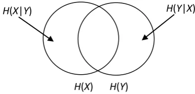
From the information-theory point of view, the potential gain from exploiting the temporal domain correlation can be estimated by quantifying the entropy relationship between two temporally dependent images (Fig. 1). An efficient data distribution system ensures that the reduced entropy is less than the original entropy. As the entropy is the measurement of the number of bits required to transmit data, reducing the entropy of the transmitted data ensures savings in both storage and bandwidth. According to the information theory, “conditioning reduces uncertainty”; in other words, knowing one of the variables reduces the average uncertainty about the others in two dependent events. If X and Y are temporally dependent images, Yconveys as much information about X

as X conveys about Y. Therefore, conditioning provides additional information about the outcome of Yif the outcome of Xis known. Now, if X is the previous image of the sequence and Y the current one, conditioning Ywith X will (usually) produce a bit stream with a smaller bit rate compared with the original bit rate [11]. However, one of the concerns regarding the de-correlation process of a transmission system that could reduce its overall temporal gain is how efficiently is Y modelled using X? Sometimes, a poor mathematical model can lead to a bit rate equal to the original bit rate of Y. The next concern is how much overhead is required to send the model parameters in order to reconstruct the image at the receiver? Sometimes, modelling can greatly reduce the transmitted data but significantly increase the overhead costs which eventually decreases the total gain.

Fig. 1 Temporal uncertainty reduction for image X and Y.

Another concern is that how co-dependent are Yand X? This reflects the fact that, if the geographical diversity between the images is huge, conditioning will not greatly reduce the uncertainty. Most multispectral data contain redundant information caused by the correlations among pixels and spectral bands. Therefore, to avoid sending repeated information, and to better utilise the transmission bandwidth, data reduction is required and possible. Data reduction for distribution is achieved through a process of redundancy removal or de-correlation. Statistical or transformation modeling is used to achieve the lowest possible entropy of the data which is then ready to be coded or transmitted. Basically, data values/symbols with high probabilities are coded with fewer bits than those with low probabilities.

3.

UNCERTAINTY MEASUREMENT

The entropy is a measure of the average uncertainty in the random variable. The key measure of energy or variance outcome is known as entropy, since it indicates the lowest possible average number of bits needed for the storage and transmission of the image, after an appropriate coding technique, such as Huffman coding, is applied. Entropy is the

minimum descriptive complexity of a random variable, and mutual information is the communication rate in the presence of noise. Let xi be a data set over a space, X, so xiÎ{X}

where i=1 to n. The entropy of xiis the function of its

distribution. If P(.) is the probability mass function defined overX, the entropy of Xis

H(X)= p(xi)log2 1

p(xi) i=1

n

å

It is dependent upon the probability of the distribution of the pixel values and not on the actual values. Entropy is sensitive to the data range and, the number of symbols and categories, but not to the actual values.

Now, the conditional entropyH(Y|X) , which is the entropy of a random variable conditional on the knowledge of another random variable, can be estimated from multi-temporal prediction [1]. After a good prediction model is applied, most image prediction errors can be very closely approximated by the symmetric exponential distribution. The entropy of this kind of distribution is a monotonic function of its variance: The smaller the variance, the smaller the entropy [12]. Minimisation of the SSE (sum squared error) for regression analysis means minimising the variance of the prediction error. The reduction in uncertainty due to another random variable is called the mutual information. For two random variables X and Y this reduction is the mutual information

MI(X:Y)=H(X)-H(Y|X) _{(2) MI(X:Y)=MI(Y:X)= p(x,y)log}

2

p(y,x)

p(y)p(x)

xÎX

å

yÎY

å

4.

GEOGRAPHICAL DIVERSITY OF

MULTI-TEMPORAL IMAGES

Sensors installed in the satellite are developing day by day and the resolution of taking the images have gained a dominant level. Spatial resolution refers to the size corresponding to the ground area covered by a pixel and 15-80 metres, such as that of the Landsat ETM+ (enhanced thematic mapper) considered medium resolution. This multispectral image collects data in eight bands within the spectral range of 0.45 µm to 2.35 µm, which include one panchromatic and one thermal bands of lower resolution. Among them, Band1 (blue) is used for atmospheric and deep-water imaging; Band2 (green) is used for imaging of vegetation and deep water structures; Band3 (red) is used for imaging of man-made objects, soil, and vegetation; band4 (near IR) is used for such things as vegetation and biomass surveys;Band5 (short wave IR) is used for such things as to sense vegetation moisture and snow/cloud reflectance differences and Band7 (short wave IR) is used for such things as determining vegetation moisture and depiction of minerals (based on hydroxyl ions) for geological mapping.

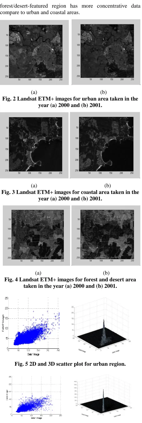
In the proposed experiment, three pair of Landsat ETM+ images of the Australia were taken where each pair are one year apart (Fig. 2, Fig. 3 and Fig.4). One is taken in the year 2000 and the other is taken in the year 2001. The three pair was specially chosen considering distinct features of urban, coastal and forest/desert areas. At first the distinguish nature of the three different pair of Landsat images has been illustrated with their 2D and 3D scatter plot. As can be seen from Fig. 5, Fig. 6 and Fig. 7 the urban, coastal and forest or desert areas respectively. It can be apparently seen that the

H

(

Y

|

X

)

H

(

X

|

Y

)

forest/desert-featured region has more concentrative data compare to urban and coastal areas.

(a) (b)

Fig. 2 Landsat ETM+ images for urban area taken in the year (a) 2000 and (b) 2001.

(a) (b)

Fig. 3 Landsat ETM+ images for coastal area taken in the year (a) 2000 and (b) 2001.

(a) (b)

Fig. 4 Landsat ETM+ images for forest and desert area taken in the year (a) 2000 and (b) 2001.

Fig. 5 2D and 3D scatter plot for urban region.

Fig. 6 2D and 3D scatter plot for coastal region.

Fig. 7 2D and 3D scatter plot for desert/forest region.

5.

RESULTS AND DISCUSSION

Table 1 and Table 2 have depicted the original entropy of the band wise images for the year 2000 and 2001 respectively. Now the main observation is that the H(Y_{) is less informative} thanH(X).It can be justified by the fact that the pixel values of the images in the year 2001 have narrow range. It is due to the fact that the imaging conditions of the two images are completely different as far as environmental or weather factors are concerned.

Table 1. Original Entropy for the Year 2000 (H(X))

Bands Coastal Forest/Desert Urban

Band1 4.7848 4.9000 5.4360 Band2 _{4.7957 5.2937 5.7103} Band3 _{5.0806 5.9286 6.2642} Band4 _{5.6279 5.1332 5.6112} Band5 _{6.1878 6.9435 6.7542}

Band7 _{5.5793 6.4436 6.3253}

Table 2. Original Entropy for the Year 2001 (H(Y))

Bands Coastal Forest/Desert Urban

Band1 3.8633 4.0394 4.6336

Band2 _{4.3307 4.3746 4.9165} Band3 _{4.7385 5.0302 5.4671} Band4 _{5.4479 5.0115 5.5835} Band5 _{5.3779 6.2322 6.1553} Band7 _4.8722 5.6134 _5.6719

Fig. 8 Entropy difference between the two images.

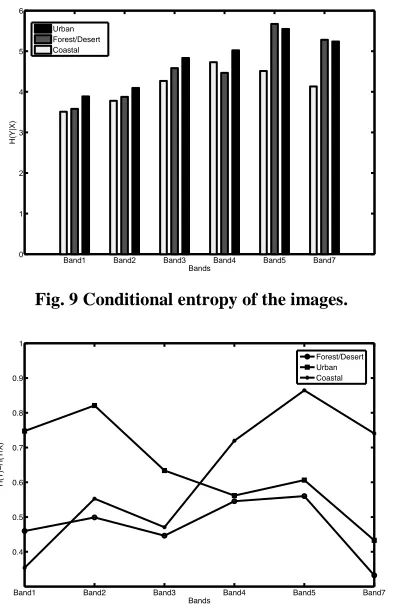
Now the conditional entropy H(Y|X) is given in Fig. 9. This is the entropy of one image having the knowledge of other. This has been extensively studied by applying a linear prediction algorithm to predict the recent image from reference image and then residual entropy has been calculated [13]. The plot easily depicts the fact that the urban areas have the most potentiality to remove the temporal correlation by applying prediction algorithm. Because the features in the urban areas like concrete, bare fields, roads, grass and trees are temporally very much co-dependent.

Fig. 9 Conditional entropy of the images.

Fig. 10 Uncertainty reduction of the image bands.

Finally the reduction of uncertainty for conditioning has been given in Fig. 10. Every case of feature has the potentiality to reduce the entropy, ultimately the transmitted data. In some bands urban areas are more compressible than the other two feature of region.

6.

CONCLUSSION

The general idea is that, rather than a complete image having to be transmitted each time (even with compression), the most recent images can be predicted from those that have already been received. After a good prediction model is applied, most image prediction errors can be very closely approximated by the symmetric exponential distribution of the entropy function. The entropy of this kind of distribution is a monotonic function of its variance: The smaller the variance, the smaller the entropy. As can be implied from the taken images that there is not much real changed areas over the time. So the correlation remains unchanged as well as the total variance. Consequently it can be said that the correlation is invariance to the features diversity. So all images have equal opportunity for entropy reduction procedure by conditioning. The multi-temporal image conditioning needs to be further exploited in this respect for efficient transmission of satellite images. Future extension of this work will explore the comparative analysis of temporal image conditioning.

7.

ACKNOWLEDGMENTS

Our special thanks to Dr. Xiuping Jia for providing us with the LANDSAT images.

8.

REFERENCES

[1] M. A. Mamun, X. Jia and M. Ryan, “Adaptive Data Compression for Efficient Sequential Transmission and Change Updating of Remote Sensing Images”, IEEE Geoscience and Remote Sensing Symposium (IGARSS ‘09), Cape Town, South Africa, pp. 498-501 (IV), July 2009.

[2] Richards, J. A. and Jia, X. 2006. Remote Sensing and Digital Analysis, Springer Verlag.

[3] W. Zhu, X. Tian, F. Zhou and Y. Chen, "Fast disparity estimation using spatio-temporal correlation of disparity field for multiview video coding." IEEE Transactions on Consumer Electronics, vol. 56(2), pp. 957-964, 2010. [4] K. Peleg and G. L. Anderson, "FFT regression and

cross-noise reduction for comparing images in remote sensing." International Journal of Remote Sensing, vol. 23(10), pp. 2097-2124, 2002.

[5] G. B. Cai, C. O. Davis and A. F. H. Goetz, "A Review of Atmospheric Correction Techniques for Hyperspectral Remote Sensing of Land Surfaces and Ocean Color." IEEE International Conference on Geoscience and Remote Sensing Symposium (IGARSS '06), pp. 1979-1981, 2006.

[6] G. Bo-Cai, M. J. Montes, L. Rong-Rong, H. M. Dierssen and C. O. Davis, "An Atmospheric Correction Algorithm for Remote Sensing of Bright Coastal Waters Using MODIS Land and Ocean Channels in the Solar Spectral Region." IEEE Transactions on Geoscience and Remote Sensing, vol. 45(6), pp. 1835-1843, 2007.

[7] M. Tunay and A. Atesoglu, "Effect of atmospheric correction for different land use on Landsat 7 ETM+ satellite imagery." Presented at 4th International Conference on Recent Advances in Space Technologies (RAST '09), 2009.

[8] P. Tyagi and U. Bhosle, "Image based atmospheric correction of remotely sensed images." International Conference on Computer Applications and Industrial Electronics (ICCAIE), pp. 63-68, 2010.

Band1 Band2 Band3 Band4 Band5 Band7 0

1 2 3 4 5 6

Bands

H

(Y

|X

)

[9] Z. Wei, D. Qian and J. E. Fowler, "Multitemporal hyperspectral image compression." IEEE Geoscience and Remote Sensing Letters, vol. 8(3), pp. 416-420, 2011. [10]M. Mamun, X. Jia and M. J. Ryan, “Nonlinear Elastic

Model for Flexible Prediction of Remotely Sensed Multitemporal Images”, IEEE Geoscience and Remote Sensing Letters, vol. 11, no. 5, pp. 1005 – 1009, 2013. [11]Fowler, J. E., and Rucker, J. T. 2007 3-D wavelet-based

compression of hyperspectral imagery in C.-I. Chang and

E. Hoboken, (eds.), Hyperspectral Data Exploitation: Theory and Applications. NJ: Wiley, pp. 379–407 [12]Cover, T. M. and Thomas, J. A. 2006 Elements of

Information Theory, 2nd Ed., John Wiley & Sons, Hoboken New Jersey.