Application of Hidden Markov Models
and Hidden Semi-Markov Models to
Financial Time Series
Bulla, Jan
Georg-August-Universität Göttingen
2006
Online at
https://mpra.ub.uni-muenchen.de/7675/
Dissertation
Presented for the Degree of Doctor of Philosophy at the Faculty of Economics and Business Administration
of the Georg-August-University of G¨ottingen
by
Jan Bulla from
Hannover, Germany
1 Introduction 1
2 Hidden Markov Models 6
2.1 Fundamentals . . . 7
2.1.1 Independent Mixture Distributions . . . 7
2.1.2 Markov Chains . . . 14
2.2 Hidden Markov Models . . . 16
2.2.1 The basic Hidden Markov Model . . . 16
2.2.2 The Likelihood of a Hidden Markov Model . . . 18
3 Parameter Estimation for Hidden Markov Models 20 3.1 Estimation Algorithms for Stationary Hidden Markov Models . . . 21
3.1.1 Direct Numerical Maximization . . . 21
3.1.2 The Stationary EM Algorithm . . . 23
3.1.3 The Hybrid Algorithm . . . 25
3.2 A simulation experiment . . . 25
3.2.1 Study design . . . 26
3.2.2 Results for different parameterizations . . . 26
3.2.3 Performance of the hybrid algorithm . . . 29
3.2.4 Coverage probability of confidence intervals . . . 32
3.3 An application . . . 35
4 Markov Switching Approaches to Model Time-Varying Betas 38
4.1 The Unconditional Beta in the CAPM . . . 40
4.2 The Markov Switching Approach . . . 41
4.3 Data and Preliminary Analysis . . . 43
4.3.1 Data Series . . . 43
4.3.2 Univariate Statistics . . . 44
4.4 Empirical Results . . . 45
4.4.1 Unconditional Beta Estimates . . . 45
4.4.2 Modeling Conditional Betas . . . 46
4.4.3 Comparison of Conditional Beta Estimates . . . 46
4.4.4 In-Sample and Out-Of-Sample Forecasting Accuracy . . 48
4.5 Conclusion . . . 50
4.6 Estimation Results . . . 52
5 Hidden Semi-Markov Models 57 5.1 The Basic Definitions . . . 58
5.1.1 Semi-Markov Chains . . . 59
5.1.2 Hidden Semi-Markov Models . . . 61
5.2 The Likelihood Function of a Hidden Semi-Markov Model . . . 62
5.2.1 The Partial Likelihood Estimator . . . 64
5.2.2 The Complete Likelihood Estimator . . . 66
5.3 The EM Algorithm for Hidden Semi-Markov Models . . . 67
5.3.1 The Q-Function . . . 68
5.3.2 The Forward-Backward Algorithm . . . 72
5.3.2.1 The Forward Iteration . . . 75
5.3.2.2 The Backward Iteration . . . 77
5.3.3 The Sojourn Time Distribution . . . 80
5.3.3.2 The Q-Function based on the Partial
Likeli-hood Estimator . . . 83
5.3.4 Parameter Re-estimation . . . 84
5.3.4.1 The Initial Parameters . . . 85
5.3.4.2 The Transition Probabilities . . . 85
5.3.4.3 The State Occupancy Distribution . . . 86
5.3.4.4 The Observation Component . . . 94
5.4 Asymptotic properties of the maximum likelihood estimators . . . 105
5.5 Stationary Hidden Semi-Markov Models . . . 105
6 Stylized Facts of Daily Return Series and Hidden Semi-Markov Models 107 6.1 Modeling Daily Return Series . . . 108
6.2 The Data Series . . . 109
6.3 Empirical Results . . . 110
6.4 Conclusion . . . 120
6.5 Estimation Results . . . 121
7 Conclusion and Future Work 124 A The EM Algorithm 126 A.1 Prerequisites . . . 126
A.2 Implementation of the EM Algorithm . . . 128
A.3 Convergence properties of the EM Algorithm . . . 129
B The Forward-Backward Algorithm 131
C Source Code for the Estimation Procedures 135
1.1 Basic structure of a Hidden Markov Model . . . 1
1.2 Basic structure of a Hidden Semi-Markov Model . . . 2
2.1 Process structure of a two-component mixture distribution . . . 8
2.2 Percentage return of the DAX 30, DJ STOXX, and FTSE 100 Index . . . 11
2.3 Histogram of daily returns of the DAX 30, DJ STOXX, and FTSE 100 Index with fitted normal distributions . . . 12
2.4 Histogram of daily returns of the DAX 30, DJ STOXX, and FTSE 100 Index with fitted mixtures of normal distributions . . 13
2.5 Basic structure of a Hidden Markov Model . . . 17
2.6 Process structure of a two-state Hidden Markov Model . . . 18
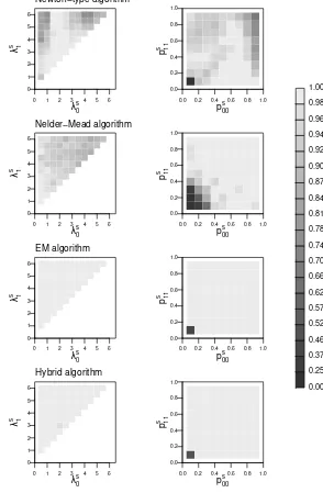
3.1 Proportion of successful estimations for specific combinations of the parameter starting values using the Nelder-Mead algorithm and different parameterizations of the state-dependent parame-ters. . . 27
3.2 Effect of the stopping criterionǫin the hybrid algorithm on the number of EM iterations, relative toǫ= 10−5 . . . 29
3.3 Proportion of successful estimations for specific combinations of the parameter starting values using different algorithms for parameter estimation . . . 31
3.4 Coverage probabilities of bootstrap confidence intervals with dif-ferent levels of confidence for series simulated using λ2, i.e. a
3.5 Coverage probabilities of bootstrap confidence intervals with dif-ferent levels of confidence for series simulated using λ1, i.e. a
small difference between the state-dependent parameters . . . . 34
3.6 Scaled computational time and percentage of trials with con-vergence to the global maximum using different algorithms for parameter estimation of the quakes series . . . 36
4.1 Various conditional betas for the Media and the Technology sector 47 4.2 In-sample rank correlation coefficients . . . 49
4.3 Out-of-sample rank correlation coefficients . . . 50
5.1 Basic structure of a Hidden Semi-Markov Model . . . 62
6.1 Observed and fitted distributions for the Food sector . . . 112
6.2 Observed and fitted distributions for the Industrials sector . . . 112
6.3 Observed and fitted distributions for the Travel & Leisure sector 113 6.4 Mean and standard deviation of the sojourn time distributions of the sectors, grouped by model and high-risk (HR)/low-risk (LR) state . . . 115
6.5 Mean and standard deviation of the sojourn times . . . 115
6.6 Empirical (gray bars) and model ACF for the first six sectors at lag 1 to 100 . . . 117
6.7 Empirical (gray bars) and model ACF for the sectors seven to twelve at lag 1 to 100 . . . 118
3.1 Performance of the Newton-type and Nelder-Mead algorithms with different parameterizations of the state-dependent
param-eters . . . 26
3.2 Performance of the algorithms considered . . . 30
4.1 Descriptive statistics of weekly excess returns . . . 44
4.2 OLS estimates of excess market model . . . 52
4.3 Parameter estimates for MS models . . . 53
4.4 Parameter estimates for MS models . . . 54
4.5 Comparison of OLS betas and various conditional beta series . . 55
4.6 Comparison of OLS betas and various conditional beta series . . 56
6.1 Descriptive statistics of daily sector returns . . . 110
6.2 Standard deviation of the data and the fitted models . . . 111
6.3 Kurtosis of the data and the fitted models . . . 114
6.4 Average mean squared error and weighed mean squared error for the ACF of the 18 sectors . . . 116
6.5 Parameter estimates for the HMM . . . 121
6.6 Parameter estimates for the HSMM with normal conditional distributions . . . 122
Acknowledgements
First of all, I would like to thank my thesis advisor, Prof. Walter Zucchini, for his academic support and the Center for Statistics as well as the Friedrich-Ebert Stiftung for their financial support.
Moreover, I would also like to render my thanks to the members of the Insti-tute for Statistics and Econometrics and the Centre for Statistics at G¨ottingen. Thanks are also due especially to Daniel Adler, Oleg Nenadic, Richard Sachsen-hausen and Karthinathan Thangavelu who provided constant help and support for my work and answered all my boring questions. I owe special thanks to my co-authors Andreas Berzel and Sascha Mergner who spent numerous hours on our joint research. I would like to sincerely thank Prof. Peter Thomson and Dr. Yann Gu´edon for their inspiring comments on my work with Hidden Semi-Markov Models.
I am also indebted to the office staff, in particular Hertha Zimmer from the Institute for Mathematical Stochastics for her exceptional help in all admin-istrative matters. I greatly appreciate the financial support of Prof. Manfred Denker and Prof. Hartje Kriete who offered me the chance to participate in inspiring conferences and delicious wine-tasting sessions in Australia and New Zealand.
Introduction
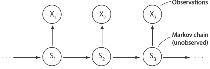
Hidden Markov Models (HMMs) and Hidden Semi-Markov Models (HSMMs) provide flexible, general-purpose models for univariate and multivariate time series, especially for discrete-valued series, categorical series, circular-valued series and many other types of observations. They can be considered as a special class of mixture models. The common properties of HMMs and HSMMs are, first of all, that both are built from two stochastic processes: an observed process and an underlying ‘hidden’ (unobserved) process. The basic structure of HMMs and HSMMs is illustrated in Figures 1.1 and 1.2, respectively.
Figure 1.1: Basic structure of a Hidden Markov Model
X
1
S
1X
2
S
2X
3
S
3. . . . . .
Observations
Markov chain (unobserved)
The models are a combination of the following two processes:
• a (semi-)Markov chainSt which determines the state at time t, and
on the current state ofSt.
Moreover, they fulfill the so-called conditional independence property: Given the hidden state at time t, the distribution of the observation at this time is fully determined. A very important consequence of these assumptions is the correlation structure of the observed data. While the autocorrelation function of HMMs is of a particular shape due to the Markov-property of the hidden process, that of the HSMM is more flexible and offers a large variety of possible temporal dependence structures.
Figure 1.2: Basic structure of a Hidden Semi-Markov Model
X1
S1 X
. . . X
S2 X
. . .
. . . . . .
Markov chain (unobserved) Observations, number of observations: sojourn time distribution
n+1
n n+m
~ ~
HMMs and HSMMs have been used for more than two decades in signal-processing applications, especially in the context of automatic speech recog-nition (e.g. Ferguson 1980, Rabiner 1989). In this context, they allow one to make inferences about the unobserved process. In economic time series mod-eling, the regime-switching models based on the seminal works of Hamilton (1989, 1990) are a very well-known application of HMMs. Another application is described in the widely known article of Ryd´en et al. (1998) who analyzed the variation of a daily return series from the S&P 500 index by a HMM.
numerous articles on theoretical and practical aspects have been published, several gaps remain. This thesis addresses some of them, divided into three main topics:
1. Computational issues in parameter estimation of stationary hidden Markov models.
2. A Markov switching approach to model time-varying Beta risk of pan-European Industry portfolios.
3. Stylized facts of financial time series and HSMMs.
The decision to work on the first topic was motivated by the fact that the parameters of a HMM can be estimated by direct numerical maximization (DNM) of the log-likelihood function or, more popularly, using the expectation-maximization (EM) algorithm. Although neither of the algorithms is superior to the other in all respects, researchers and practitioners who work with HMMs tend to use only one of the two, and to ignore the other. We compared the two methods in terms of their speed of convergence, effect of different model parameterizations, how the fitted-log likelihood depends on the true parameter values and on the starting values of the algorithms. Further, it is desirable to fit a stationary HMM in many applications. However, the standard form of the EM algorithm is not designed to do this and therefore, in most cases, au-thors who use it fit homogeneous but non-stationary models instead. We show how the EM algorithm could be modified to fit stationary HMMs. We propose a hybrid algorithm that is designed to combine the advantageous features of the EM and DNM algorithms, and compare the performance of the three al-gorithms (EM, DNM and the hybrid) using simulated data from a designed experiment, and also a real data set. We then describe the results of an ex-periment to assess the true coverage probability of bootstrap-based confidence intervals for the parameters.
The results of the comparison of the EM algorithm and DNM clearly show the trade-off between stability and performance. The hybrid algorithm seems to provide an excellent compromise; it is as stable as the EM-algorithm but it converges faster. Further, we show that the true coverage probability for bootstrap-based confidence intervals, obtained by parametric bootstrap, may be unreliable for models whose state-dependent parameters lie close to each other.
financial time series. The modeling of daily return series with HMMs has been investigated by several authors. After the seminal work of Ryd´en et al. (1998) who showed that the temporal and distributional properties of daily returns series are well reproduced by the two- and three-state HMMs with normal components, several other authors followed their ideas (see, e.g., Cecchetti et al. 1990, Linne 2002, Bialkowski 2003).
For many applications it is desirable to model a portfolio comprising multiple assets, e.g., a portfolio of European shares selected from the Dow Jones EURO STOXX 600. Fitting a multivariate HMM with normal component distribu-tions would require the estimation of the covariance matrix for each of the states. In the worst case, considering the portfolio of a professional investor which is composed of all 600 shares, the procedure would involve a matrix of dimension 600×600 yielding 180300 parameters to be estimated for each state. It is obvious that such a model would be grossly over-parameterized, resulting in unreliable estimates.
A possible solution to the quadratic increase of the number of parameters is based on the Capital Asset Pricing Model (CAPM). In this model, the return of each asset is linearly dependent to the market return (plus an error term):
Rit =αi+βiR0t+ǫit, ǫit ∼N(0, σi2),
whereRit, R0tare the returns of the ith asset and the market, respectively. The
error term is represented by ǫit; βi is the market or systematic risk. In this
setup, the number of parameters increases only linearly with the number of assets considered. The joint behavior of all assets is modeled by the common dependence on the market return.
We study the performance of two Markov switching models based on the ap-proaches of Fridman (1994) and Huang (2000), and compare their forecast performances to three models, namely a bivariate t-GARCH(1,1) model, two Kalman filter based approaches and a bivariate stochastic volatility model. The main results of the comparisons indicate that the random walk process in connection with the Kalman filter is the preferred model to describe and forecast the time-varying behavior of sector betas in a European context, while the two proposed Markov switching models yielded unsatisfactory results.
several problems related to hidden semi-Markov chains were further investi-gated by different authors, e.g., Levinson (1986), Gu´edon & Cocozza-Thivent (1990), Gu´edon (2003), Sansom & Thomson (2001), Yu & Kobayashi (2003) and different parametric hypotheses were considered for the state occupancy, as well as for the distribution of the observations. We provide estimation pro-cedures for a variety of HSMMs belonging to the recently introduced class of right-censored HSMMs. In contrast to the original model of Ferguson (1980), they do not require the assumption that the end of a sequence systematically coincides with the exit from a state. Such an assumption is unrealistic for many financial time series, daily return series in particular.
The ability of a HMM to reproduce several stylized facts of daily return se-ries was illustrated by Ryd´en et al. (1998). However, they point out that one stylized fact cannot be reproduced by a HMM, namely the slowly decaying autocorrelation function of squared returns, which plays a key role in risk-measurement and the pricing of derivatives. The lack of flexibility of a HMM to model this temporal higher order dependence can be explained by the im-plicit geometric distributed sojourn time in the hidden states.
We present two alternative HSMM-based approaches to model eighteen series of daily sector returns with about 5000 observations. Our key result is that the slowly decaying autocorrelation function is significantly better described by a HSMM with negative binomial sojourn time and normal conditional dis-tributions.
Hidden Markov Models
Hidden Markov Models (HMMs) are a class of models in which the distribu-tion that generates an observadistribu-tion depends on the state of an underlying but unobserved Markov process. In this chapter we provide a brief introduction to HMMs and explain the basics of the underlying theory.
HMMs have been applied in the field of signal-processing for more than two decades, especially in the context of automatic speech recognition. However, they also provide flexible, general-purpose models for univariate and multi-variate time series, including discrete-valued series, categorical series, circular-valued series and many other types of observations. Consequently, the interest in the theory and applications of HMMs is rapidly expanding to other fields, e.g.:
• Various kinds of recognition: faces, speech, gesture, handwriting/signature.
• Bioinformatics: biological sequence analysis.
• Environment: wind direction, rainfall, earthquakes.
• Finance: daily return series.
The bibliography lists several articles and monographs that deal with the ap-plication of HMMs in these fields. Important references include Durbin et al. (1998), Elliott et al. (1995), Ephraim & Merhav (2002), Koski (2001), Rabiner (1989).
• Availability of all moments: mean, variance, autocorrelations.
• The likelihood is easy to compute; the computation is linear in the
num-ber of observations.
• The marginal distributions are easy to determine and missing
observa-tions can be handled with minor effort.
• The conditional distributions are available, outlier identification is
pos-sible and forecast distributions can be calculated.
In addition, HMMs are interpretable in many cases and can easily accommo-date additional covariates. Furthermore, they are moderately parsimonious; in many applications a simple two-state model provides a reasonable fit.
This chapter is organized as follows. In Section 2.1 we introduce indepen-dent mixture models and discrete Markov chains, the two main components of HMMs. Subsequently in Section 2.2, we present the construction of a HMM and show how the likelihood can be calculated.
2.1
Fundamentals
This section provides a brief introduction to two fundamental concepts that are necessary to understand the basic structure of Hidden Markov Models (HMMs). As the marginal distribution of a HMM is a discrete mixture model, we first provide a general outline of mixture distributions in Section 2.1.1. Then, we introduce Markov chains in Section 2.1.2 since the selection process of the parameters of a HMM is modeled by a Markov chain.
2.1.1
Independent Mixture Distributions
In general, an independent mixture distribution consists of a certain number of
component conditional distributions. In some applications it isi reason-able to assume that the population heterogeneity is modeled by a continuous mixture. More details on continuous mixtures can be found, e.g., in B¨ohning (1999).
the mixture distribution is characterized by the two random variablesX0 and
X1along with their probability functions or probability density functions (pdf).
Random variable Probability function pdf
X0 p0(x) f0(x)
X1 p1(x) f1(x)
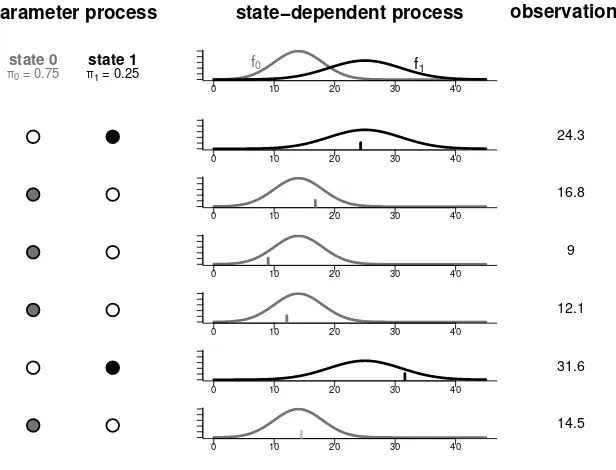
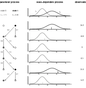
Moreover, for theparameter processa discrete random variableS is needed to perform the mixture:
S :=
0 with probability π0
1 with probability π1 = 1−π0 .
One may imagine S like tossing a coin: If S takes the value 0, then an obser-vation is a realization of X0; if S takes the value 1, then an observation is a
realization ofX1. The structure of that process for the case of two continuous
[image:19.595.175.483.443.678.2]component distributions is shown in Figure 2.1.
Figure 2.1: Process structure of a two-component mixture distribution
parameter process
state 0 state 1
π0 = 0.75 π1 = 0.25
state−dependent process
0 10 20 30 40
f0 f1
0 10 20 30 40
0 10 20 30 40
0 10 20 30 40
0 10 20 30 40
0 10 20 30 40
0 10 20 30 40
observations
24.3
16.8
9
12.1
31.6
14.5
they cannot be assigned to a distinct random variable.
Given the probability of each component and the respective probability dis-tributions, the probability density function of the mixture can be computed easily. For ease of notation we only treat the continuous case. Let X denote the outcome of the mixture. Then, its probability density function is given by
f(x) = π0f0(x) +π1f1(x).
The extension to the J-component case is straightforward. Let π0, . . . , πJ−1
denote the weights assigned to the different components and f0, . . . , fJ−1
de-note their corresponding probability density functions. Then, the distribution of the outcome, X, is a mixture and can be easily calculated as a linear com-bination of the component distributions:
f(x) =
J−1
X
i=0
πifi(x).
Moreover, the calculation of the k-th moment E(Xk) is simply a linear
com-bination of the respective moments of its components:
E(Xk) =
J−1
X
i=0
πiE(Xik), k ∈ {1,2, ...}.
Note that this does not hold for the central moments, e.g., the variance of a mixture:
V ar(X)6=
J−1
X
i=1
πiV ar(Xi).
The estimation of the parameters of a mixture distribution is usually performed by a maximum likelihood (ML) algorithm. The likelihood of a mixture model with J components is given by
L(θ0, . . . , θJ−1, π0, . . . , πJ−1, x0, . . . , xτ−1) =
τ−1
Y
j=0
J−1
X
i=0
πifi(xj, θi).
where θ0, . . . , θJ−1 are the parameter vectors of the component distributions,
It is not possible to maximize this likelihood function analytically. Therefore, the parameter estimation has to be carried out by numerical maximization of the likelihood using special software. A very useful software package for the estimation of mixture models is C.A.MAN, developed by B¨ohning et al. (1992).1
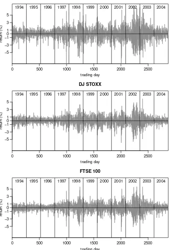
One example in which mixture distributions with continuous components can be applied is the analysis of stock returns, as demonstrated in the following example. Figure 2.2 shows the daily percentage returns of the DAX 30, DJ STOXX, and FTSE 100 Index between 1st January 1994 and 31st December 2004.
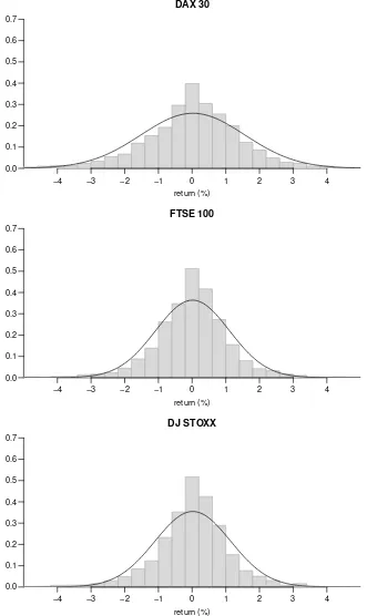
It is visible that the variance of the returns is not constant over the whole trading period. Instead, there are some periods with low absolute returns and others with high absolute returns – there is “volatility clustering” observable for many financial time series. For that reason, a simple normal distribution does not provide an adequate description of the daily percentage return on the indices, as can be seen in Figure 2.3, which shows a histogram of the daily returns and a fitted normal distribution.
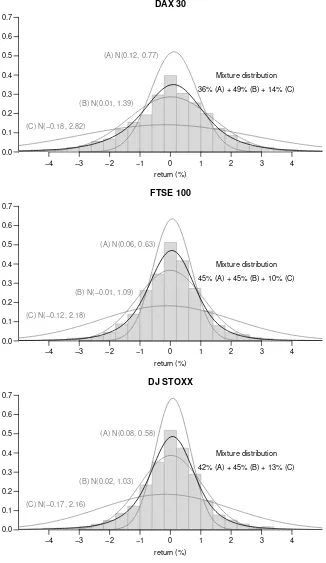
The fitted normal distribution underestimates the probability of extremely low and high absolute returns. The return series also shows excess kurtosis compared to the normal distribution. In contrast, a mixture of three normal distributions as shown in Figure 2.4 provides a better fit. The mixing weights correspond to those obtained by fitting a HMM.
1
Figure 2.2: Percentage return of the DAX 30, DJ STOXX, and FTSE 100 Index
0 500 1000 1500 2000 2500
−5 0 5
DAX 30
trading day
return (%)
−3 −1 1 3
1994 1995 1996 1997 1998 1999 2000 2001 2002 2003 2004
0 500 1000 1500 2000 2500
−5 0 5
DJ STOXX
trading day
return (%)
−3 −1 1 3
1994 1995 1996 1997 1998 1999 2000 2001 2002 2003 2004
0 500 1000 1500 2000 2500
−5 0 5
FTSE 100
trading day
return (%)
−3 −1 1 3
Figure 2.3: Histogram of daily returns of the DAX 30, DJ STOXX, and FTSE 100 Index with fitted normal distributions
return (%)
−4 −2 0 2 4
0.0 0.1 0.2 0.3 0.4 0.5 0.6 0.7
DAX 30
−3 −1 1 3
return (%)
−4 −2 0 2 4
0.0 0.1 0.2 0.3 0.4 0.5 0.6 0.7
FTSE 100
−3 −1 1 3
return (%)
−4 −2 0 2 4
0.0 0.1 0.2 0.3 0.4 0.5 0.6 0.7
DJ STOXX
Figure 2.4: Histogram of daily returns of the DAX 30, DJ STOXX, and FTSE 100 Index with fitted mixtures of normal distributions
return (%)
−4 −2 0 2 4
0.0 0.1 0.2 0.3 0.4 0.5 0.6 0.7
DAX 30
−3 −1 1 3
(A) N(0.12, 0.77)
(B) N(0.01, 1.39)
(C) N(−0.18, 2.82)
Mixture distribution
36% (A) + 49% (B) + 14% (C)
return (%)
−4 −2 0 2 4
0.0 0.1 0.2 0.3 0.4 0.5 0.6 0.7
FTSE 100
−3 −1 1 3
(A) N(0.06, 0.63)
(B) N(−0.01, 1.09)
(C) N(−0.12, 2.18)
Mixture distribution
45% (A) + 45% (B) + 10% (C)
return (%)
−4 −2 0 2 4
0.0 0.1 0.2 0.3 0.4 0.5 0.6 0.7
DJ STOXX
−3 −1 1 3
(A) N(0.08, 0.58)
(B) N(0.02, 1.03)
(C) N(−0.17, 2.16)
Mixture distribution
2.1.2
Markov Chains
As the theory of Markov chains is well documented, we present only a short introduction to the topic and some of their basic properties that are necessary for the construction of HMMs. For a detailed description of Markov chains see, e.g., Grimmett & Stirzaker (2001) or Parzen (1962).
Consider a stochastic process, i.e. a sequence of random variables {St : t ∈
0,1, . . .} taking values in the state space {0, . . . , J −1}. For more general Markov processes, the time and state space may also be continuous. However, for this work we deal only with discrete-time Markov processes with discrete state space. Such processes are called Markov chains.
A stochastic process {St} is a Markov process if, roughly speaking, given the
current state of the processSt, the futureSt+1 is independent of its pastSt−1,
St−2,...,S0. More precisely, lets0, . . . , st, st+1denote a sequence of observations
of a stochastic process {St, t = 0,1, . . .}. {St} is a Markov process if it has
the Markov property, namely
P(St+1 =st+1|St=st, St−1 =st−1, ..., S0 =s0
| {z }
”entire history”
) =P(St+1 =st+1|St =st)
for all t∈ {0,1, . . .}.
A Markov chain is called homogeneous, or Markov chain with stationary transition probabilities pij := P(St+1 = j|St = i), if the transition
proba-bilities are independent of t. The transition probabilities of a homogeneous
J-state Markov chain can be summarized in aJ×J transition probability matrix (TPM) and can be presented as
T :=
p0 0 · · · p0J−1
..
. . .. ...
pJ−1 0 · · · pJ−1J−1
,
with pij =P(St+1 =j|St=i) and
J−1
X
j=0
pij = 1, i∈ {0, . . . , J −1}.
The TPM T contains the one-step transition probabilities and thus, describes the short-term behavior of the Markov chain. For describing the long-term behavior of a Markov chain, one can define thek-step transition probabilities
contains thek-step transition probabilities can be calculated as thekth power
of the TPM T. That is,
T(k) :=
p0 0(k) · · · p0J−1(k)
... . .. ...
pJ−1 0(k) · · · pJ−1J−1(k)
=Tk.
For a proof, see Grimmett & Stirzaker (2001).
In this context one says that state j is accessible from state i, written i →j, if the chain may ever reach state j with positive probability, starting from state i. That is, i → j if there exists some k ∈ {1,2, . . .} with pij(k) > 0.
Furthermore, states i andj communicate with each other, which is written as
i↔j, if i→j andj →i. We can then call a Markov chain to beirreducible
if i↔j for alli, j ∈ {0, . . . , J −1}. In the following, as in most applications, we assume the Markov chain to be irreducible.
The k-step transition probabilities provide the conditional probabilities to be in state j at time t+k, given that the Markov chain is in state i at time t. However, in general, the marginal probability of the Markov chain to be in state i at a given time t is also of interest. Given the probability distribution for the initial state2, π := (P(S
1 = 1), . . . , P(S1 =m)) withPmi=1πi = 1, the
distribution of the state at timet can be computed as
(P(St= 0), . . . , P(St =J −1)) =πTk−1.
If the Markov chain is homogeneous and irreducible, one can show thatπTk−1 converges to a fixed vector, sayπs, for large t. This unique vector is called the stationary distribution and can be determined by solving
πs=πsT subject to πs1′ = 1.
For a proof of this result, see Seneta (1981). A Markov chain is said to be sta-tionary, if the stationary distributionπs exists and if it describes the marginal distribution of the states for all t ∈ {0,1, . . .}. In particular, for the distri-bution of the initial state one has that π = πs. In practice, depending on
the application, one has to decide whether it is sensible to assume that the underlying Markov chain of a HMM is stationary or not.
2
2.2
Hidden Markov Models
In this section we give a brief introduction to HMMs and their basic properties. For further reading, see, e.g., Ephraim & Merhav (2002) or MacDonald & Zucchini (1997). If not indicated otherwise, we also refer to the latter as standard reference for this section.
In an independent mixture model, the sequence of hidden states as well the sequence of observations is independent by definition. If there is correlation between the states, the independent mixture is not an appropriate model any-more as it does not take account of all the information contained in the data. One way of modeling data series with serial correlation is to let the parameter selection process be driven by an unobserved (i.e. hidden) Markov chain. This approach yields the HMM, which is a special case of a dependent mixture. Different underlying processes can also be treated. For example, in Chapter 5 we generalize the parameter selection process to a semi-Markov chain, which yields the HSMMs.
2.2.1
The basic Hidden Markov Model
Let {Xt} = {Xt, t = 0,1, . . .} denote a sequence of observations and {St} =
{St, t = 0,1, . . .} a Markov chain defined on the state space {0, . . . , J −1}.
For better readability, we introduce the notation
Xt1
t0 :={Xt0, . . . , Xt1}
with t0 < t1; Stt01 is defined similarly.
Consider a stochastic process consisting of two parts: Firstly the underlying but unobserved parameter process {St}, which fulfills the Markov property
P(St = st|S1t−1 = st1−1) = P(St = st|St−1 = st−1), and secondly the
state-dependent observation process {Xt}, for which the conditional indepen-dence property
P(Xt=xt|X0t−1 =xt0−1, S0t =st0) =P(Xt =xt|St=st) (2.1)
holds. Then, the pair of stochastic processes {(St, Xt)} is called a J-state Hidden Markov Model. Equation (2.1) means that, if St is known, Xt
depends only on St and not on any previous states or observations. The basic
Figure 2.5: Basic structure of a Hidden Markov Model
X
1S
1X
2S
2X
3S
3. . . . . .
Observations
Markov chain (unobserved)
Thus a HMM is a combination of two processes, namely a Markov chain which determines the state at time t, St = st, and a state-dependent process which
generates the observation Xt =xt depending on the current state st. In most
cases a different distribution is imposed for each possible state of the state space. The Markov chain is assumed to be homogeneous and irreducible with transition probability matrix T. By the irreducibility of {St}, there exists a
unique stationary distribution of the Markov chain,π =πs (cf. Section 2.1.2).
A HMM is rather a theoretical construction. In reality, only the state-dependent process {Xt} is observed while the underlying state process {St} remains
un-known. However, in many applications there is a reasonable interpretation for the underlying states. Suppose, for example, that the daily return series introduced in Section 2.1.1 is modeled with a two-state HMM. Then the states of the underlying Markov chain may be interpreted as condition of the finan-cial market, namely a state with high volatility and a state with low volatility representing nervous and calm periods, respectively.
The process generating the observations of a stationary two-state HMM is demonstrated in Figure 2.6. Here the observed sequence equals (24.3,16.8,9,
Figure 2.6: Process structure of a two-state Hidden Markov Model
parameter process
state 0 state 1
π0 = 0.75 π1 = 0.25
0.7 0.3
0.9 0.1
0.9 0.1
0.9 0.1
0.7 0.3
state−dependent process
0 10 20 30 40
f0 f
1
0 10 20 30 40
0 10 20 30 40
0 10 20 30 40
0 10 20 30 40
0 10 20 30 40
0 10 20 30 40
observations
24.3
16.8
9
12.1
31.6
14.5
For further details on the HMM, including a derivation of the moments and marginal distributions, the treatment of outliers and missing data, forecasting, decoding and smoothing procedures we refer to the manuscript of MacDonald & Zucchini (1997).
2.2.2
The Likelihood of a Hidden Markov Model
The likelihood of a HMM can be expressed in a closed formula, even in a relatively general framework. Let θ be set of all model parameters and let P(xt) denote a diagonal matrix with the conditional probabilities bj(xt) :=
P(Xt =xt|St =j), j = 1, . . . , m on the main diagonal. Then, the likelihood
L(θ) = P({X0 =x0, . . . , Xτ−1 =xτ−1})
= πP(x0)T P(x1)T . . .T P(xτ−1)1t, (2.2)
where 1:= (1, . . . ,1).
This form of the likelihood has several appealing properties. For example, stationary as well as non-stationary models can be handled and a (local) max-imum can be found by numerical procedures such as Newton-type algorithms or via the so called EM-algorithm.
Parameter Estimation for
Hidden Markov Models
Maximum-likelihood (ML) parameter estimation in Hidden Markov Models (HMMs) can be carried out using either direct numerical maximization or the expectation maximization (EM) algorithm (Baum et al. 1970, Dempster et al. 1977). Although neither of the algorithms is superior to the other in all respects, researchers and practitioners who work with HMMs prefer to use only one of the two algorithms, and tend to ignore the other. The aim of this section is to explore the advantages and disadvantages of both estimation procedures for HMMs.
In many applications, it is desirable to fit a stationary HMM. The EM algo-rithm is not designed to do this and therefore, in most cases, authors who use the standard form of this algorithm fit homogeneous but non-stationary mod-els instead. We show how the EM algorithm can be modified to fit stationary HMMs.
Direct numerical maximization of the likelihood using Newton-type algorithms generally converges faster than the EM algorithm, especially in the neighbor-hood of a maximum. However, it requires more accurate initial values than the EM to converge at all.
We implement both the new EM algorithm as well as direct numerical maxi-mization using the software packageRand assess their performances in terms of flexibility and stability using both simulated and real data sets. In particular, we analyze the speed of convergence, the effect of different model parameteri-zations and how the fitted-log likelihood depends on the true parameter values and on the initial values of the algorithms.
of each of the two methods by using a hybrid algorithm, and compare the performance of the three algorithms using simulated data from a designed ex-periment, and then with a real data set. Such algorithms have been proposed by some authors (e.g., Lange & Weeks 1989, Redner & Walker 1984), but the efficiency of such an algorithm has not yet been reported in the context of HMMs. We fill this gap and, as a by-product of the above simulation ex-periments, we also investigate the coverage probability of bootstrap interval estimates of the parameters.
This chapter is organized as follows. In Section 3.1 we give a brief description of the two most common methods for estimating the parameters of a HMM. Furthermore, we introduce the new EM algorithm for stationary time series and the hybrid algorithm. Section 3.2 describes the design of the simulation study, the results relating to the performance of direct maximization and the EM algorithm and then of the hybrid algorithm. The coverage probability of bootstrap-based confidence intervals is also addressed. In Section 3.3 we demonstrate the advantages of the hybrid algorithm, by fitting a set of real data. Section 3.4 summarizes the main findings of the chapter and offers some concluding remarks. To keep this section short, only the main results are presented. The entire analysis of this joint work with A. Berzel can be found in Bulla & Berzel (2006).
3.1
Estimation Algorithms for
Stationary Hidden Markov Models
The parameters of HMMs are generally estimated using the method of maxi-mum-likelihood (ML). Equation (2.2) shows that the likelihood equations have a highly nonlinear structure and there is no analytical solution for the ML es-timates. The two most common approaches to estimate the parameters of a HMM are the EM algorithm and direct numerical maximization (DNM) of likelihood. In this section we present their strengths and weaknesses and in-troduce a hybrid algorithm, a combination of both. For alternative approaches including variations on ML estimation see, e.g., Archer & Titterington (2002).
3.1.1
Direct Numerical Maximization
Mac-Donald & Zucchini (1997). Recalling Equation (2.2), there exists a convenient explicit expression for the log-likelihood of a HMM that can be easily evalu-ated even for very long sequences of observations. This makes it possible to estimate the parameters by DNM of the log-likelihood function. DNM has appealing properties, especially concerning the treatment of missing observa-tions, flexibility in fitting complex models and the speed of convergence in the neighborhood of a maximum. The main disadvantage of this method is its relatively small circle of convergence.
We use the open source statistical software R (R Development Core Team 2005), version 1.9.1, which allows the integrated functionsnlm()andoptim() to perform DNM of the negative log-likelihood. The functionnlm()carries out minimization of a function using a Newton-type algorithm (Dennis & Mor´e 1977, Schnabel et al. 1985). The function optim() offers the Nelder-Mead simplex algorithm (Nelder & Mead 1965), a popular adaptive downhill sim-plex method for multidimensional unconstrained minimization, which does not require the computation of derivatives. In general, the Nelder-Mead algorithm is more stable; however, it may also get stuck in local minima and is rather slow when compared to the Newton-type minimization. In our study, we use the values of the scaling parameters proposed by Nelder & Mead (1965) and implemented those as default values in theoptim() function.
Since both the functions nlm() and the Nelder-Mead algorithm can only per-form unconstrained numerical minimization, the parameter constraints need to be taken into account by different transformation procedures. For the tran-sition probability matrix (TPM), we apply the TR-transformation described in Zucchini & MacDonald (1998). In order to meet the non-negativity con-straint of some of the parameters of the state-dependent distributions, we use different transformations and compare their performance.
For simplicity we consider a Poisson HMM; the extension to other models is straightforward. Let λi, i = 0, . . . , J −1 denote the state-dependent
parame-ters to be transformed. The simplest transformation is the natural logarithm log(λi). A second option is to make use of the fact that the ML estimates
of the parameters of the state-dependent distributions, ˆλi, can only have
sup-port points in the interval [xmin, xmax] where xmin := min{x0, . . . , xτ−1} and
xmax:= max{x0, . . . , xτ−1}(B¨ohning 1999). We can restrict the possible range
of parameter estimates to that interval by applying a logit-type transforma-tion, log ((λi−xmin)/(xmax−λi)).
state-dependent parameters themselves: (τ0, τ1, . . . , τJ−1) := (λ0, λ1−λ0, . . . , λJ−1−
λJ−2).
Since the ordering of the states can be used for both the log- and the logit-transformations, four different parameterizations have to be taken into ac-count. In the case of the ordered logit parameterization, the range of the logit-transformation has to be adopted, i.e., logτi/(xmax−Pij=0τj)
.
In the simulation study outlined in Section 3.2.2 we study the performance of these four parameterizations using both a Newton-type and the Nelder-Mead algorithm.
3.1.2
The Stationary EM Algorithm
A popular and routinely used alternative to DNM is the Baum-Welch algo-rithm, a special case of what subsequently became known as the EM algorithm. An introduction to the EM algorithm can be found in Appendix A. There ex-ists a large literature on the EM algorithm and its application to HMMs. We do not provide any details on this well-established theory and refer to Baum et al. (1970), Dempster et al. (1977), Rabiner (1989), Liporace (1982), Wu (1983).
At this stage, we wish to note that the EM algorithm, in its original imple-mentation in the context of HMMs, can be used to fit a homogeneous, but not a stationary HMM. Thus authors who apply this method of estimation are unable to maximize the likelihood under the assumption that the model is stationary, despite the fact that such an assumption is both natural and desir-able in many applications. We show that the EM algorithm can be modified, at modest computational cost, so that it is able to fit a stationary HMM.
After assigning initial values to the parameters, the EM algorithm is imple-mented by successively iterating the E-step and the M-step until convergence is achieved.
E-step: Compute the Q-function
Q(θ, θ(k)) =ElogP(X0τ−1 =xτ0−1, S0τ−1 =sτ0−1|θ)|X0τ−1=xτ0−1, θ(k),
where θ(k) is the current estimate of the parameter vector θ.
M-step: Computeθ(k+1), the parameter values that maximize the functionQ
w.r.t. θ:
θ(k+1) = argmax
θ
The feasibility of the computation of the M-step depends strongly on the con-ditional distributions of the observations. If the solution for this maximization problem cannot be obtained analytically then the maximization has to be car-ried out numerically (see, e.g., Wang & Puterman 2001). The maximization has to be executed for each M-step at considerable computational cost. Fur-thermore the rate of convergence of the EM can be very slow, namely linear in the neighborhood of a maximum (Dempster et al. 1977).
An important advantage of the EM algorithm is that (under mild conditions) the likelihood increases at each iteration, except at a stationary point (Wu 1983). Of course the increase may take one to only a local, rather than the global, maximum and thus the results do depend on the initial values of the parameters (Dunmur & Titterington 1998). Nevertheless the circle of conver-gence is relatively large compared to competing algorithms, which leads to high numerical stability in the form of robustness against poor initial values (Hathaway 1986). A major disadvantage of the EM algorithm in the context of HMMs is the lack of flexibility to fit complex models, as the E-step of the algorithm needs to be derived for each new model (Lange & Weeks 1989). The EM algorithm for HMMs given in the literature works as follows. The three additive parts of theQ-function of a HMM given by
Q(θ, θ(k)) =
J−1
X
i=0
log πiψ1(i) +
J−1
X
j=0
τ−2
X
t=0
log pijξt(i, j)
!
| {z }
(⋆)
+
τ−1
X
t=0
log bi(xt)ψt(i)
with ψt(i) := P({St=i|X0τ−1 =xτ0−1, θ})
and ξt(i, j) := P({St=i, St+1 =j|X0τ−1 =xτ0−1, θ} (3.1)
are split up in parts and maximized separately. Clearly, this procedure fits a homogeneous, but non-stationary, HMM because the individual treatment of the summands leads to an estimate ˆπ which is not the stationary distribution of ˆT. A popular way to impose stationarity is to simply neglect the first term, calculate ˆT and then set ˆπequal to the stationary distribution of ˆT. However, this approach does not lead to the exact ML estimates of the parameters, except asymptotically.
In order to estimate a stationary Markov chain, the first two summands of (3.1) marked by (⋆) have to be treated simultaneously with the stationarity constraint
at the M-Step of each iteration. T˜ denotes the matrix obtained by replacing the last column of 1−T by the vector (1, . . . ,1)T of lengthJ.
The explicit calculation of a maximizing solution of the system of equations defined by (⋆) in (3.1), and (3.2) is more difficult than it appears. Even for the simplest non-trivial HMM with two states, the system becomes intractable. To fit a stationary initial distribution, we carry out the modified M-step by embedding a numerical maximization procedure at each iteration of the EM algorithm. We note that this procedure is much more efficient than that of carrying out the entire M-step numerically. By taking the values of T of the preceding step as initial values for the maximization procedure, the EM algorithm is not slowed down significantly.
3.1.3
The Hybrid Algorithm
The relative merits of the EM algorithm and DNM have also been discussed by Campillo & Le Gland (1989) in the context of HMMs. They concluded that the EM algorithm is an interesting approach despite slow convergence, slow E-step and complicated M-step. Modifications of the EM algorithm, such as the integration of Newton-type ‘accelerators’ have been suggested to improve the rate of convergence, but these usually lead to a loss of stability and increase in complexity (Jamshidian & Jennrich 1997, Lange 1995).
An alternative approach is to use hybrid algorithms, which are constructed by combining the EM algorithm with a rapid algorithm with strong local con-vergence, in our case the Newton-type algorithm, as follows: the estimation procedure starts with the EM algorithm and switches to a Newton-type algo-rithm when a certain stopping criterion is fulfilled (Redner & Walker 1984). This leads to a new algorithm that yields the stability and large circle of con-vergence from the EM algorithm along with superlinear concon-vergence of the Newton-type algorithm in the neighborhood of the maximum.
3.2
A simulation experiment
3.2.1
Study design
The influence of these methods on the estimation results, particularly on the resulting value of the log-likelihood and the performance of the hybrid algo-rithm are studied mainly with simulated two-state Poisson HMMs. In Section 3.3 we also analyze the effects on fitting a three-state Poisson HMM to a time series of earthquake counts.
The simulated time series are of three lengths (50, 200 and 500). For each length, four different transition probability matrices, namely,
T1 =
0.9 0.1 0.1 0.9
,T2 =
0.7 0.3 0.8 0.2
,T3 =
0.2 0.8 0.8 0.2
,T4 =
0.55 0.45 0.45 0.55
,
and two different state-dependent parameter vectors λ1 = (1,2), λ2 = (2,5)
served as parameters for the generation of the observations. This 3×4×2 exper-imental design yields 24 different two-state Poisson HMMs. The realizations of these series were generated using the default random number generator in the base-library ofR, an implementation of the Mersenne-Twister (Matsumoto & Nishimura 1998).
3.2.2
Results for different parameterizations
To test the effect of the different parameterizations from Section 3.1.1, we fit HMMs to each of the 24 generated time series where the initial values are combinations of λs
0, λs1 ∈ {0.5,1,1.5, . . . , xmax}, λs0 < λs1, and ps00, ps11 ∈
{0.1,0.2, . . . ,0.9}. Table 3.1 shows the percentage of failures, i.e. those cases in which the algorithm did not converge to a solution, and the percentage of successful convergence to the global maximum for the Newton-type and the Nelder-Mead algorithm, summed over all series.
Table 3.1: Performance of the Newton-type and Nelder-Mead algorithms with different parameterizations of the state-dependent parameters
failures (%) global maximum found (%) Newton Nelder-Mead Newton Nelder-Mead
unordered log 0.17 0.00 84.3 93.0
ordered log 0.22 0.00 81.4 93.0
unordered logit 1.04 0.00 78.1 83.9
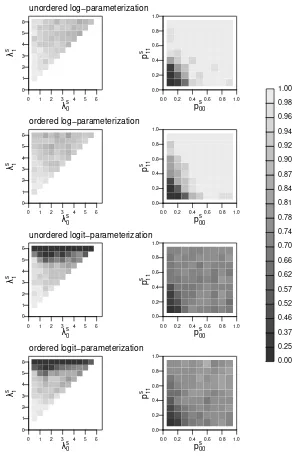
Figure 3.1: Proportion of successful estimations for specific combinations of the parameter starting values using the Nelder-Mead algorithm and different parameterizations of the state-dependent parameters.
0 1 2 3 4 5 6 0 1 2 3 4 5 6
λ0s λ1
s
unordered log−parameterization
0 1 2 3 4 5 6 0 1 2 3 4 5 6
λ0s λ1
s
ordered log−parameterization
0 1 2 3 4 5 6 0 1 2 3 4 5 6
λ0s λ1
s
unordered logit−parameterization
0 1 2 3 4 5 6 0 1 2 3 4 5 6
λ0s λ1
s
ordered logit−parameterization
0.0 0.2 0.4 0.6 0.8 1.0 0.0 0.2 0.4 0.6 0.8 1.0
p00s
p11
s
0.0 0.2 0.4 0.6 0.8 1.0 0.0 0.2 0.4 0.6 0.8 1.0
p00s
p11
s
0.0 0.2 0.4 0.6 0.8 1.0 0.0 0.2 0.4 0.6 0.8 1.0
p00s
p11
s
0.0 0.2 0.4 0.6 0.8 1.0 0.0 0.2 0.4 0.6 0.8 1.0
p00s
p11 s 0.00 0.25 0.37 0.46 0.52 0.57 0.62 0.66 0.70 0.74 0.78 0.81 0.84 0.87 0.90 0.92 0.94 0.96 0.98 1.00
of the number of failures and the convergence to the global maximum, and we will therefore apply it to all further analysis. In general, this holds true for both the Newton-type and the Mead algorithms. However, the Nelder-Mead algorithm provided better results than the Newton-type algorithm for all parameterizations, if not for each individual series.
As a typical example, Figure 3.1 demonstrates the results obtained using the Nelder-Mead algorithm and the four parameterizations for fitting a Poisson HMM to a time series with 200 observations that were simulated using the true parameters λ1 and T1 as defined above. The ML estimates obtained for
this specific series are ˆλ= (0.55,1.98)′ and ˆT with diagonal (0.89,0.97)′
lead-ing to logLmax =−333.51. Each graph in Figure 3.1 represents the proportion
of successful estimations (i.e. estimations that led to the global maximum) for specific combinations of the initial values for the state-dependent parameters,
λs
0, λs1, or the diagonal elements of the initial TPM, ps00, ps11, given a specific
parameterization of the state-dependent parameters. Light-colored areas in-dicate a high proportion of successful trials, while darker colors represent low proportions of success.
In this typical case the log-parameterization provides much more stable re-sults than does the logit-parameterization. However, the performance of all four parameterizations improves as the initial values approach the values of the maximum likelihood estimates.
The general tendency that the unordered log-parameterization provides the most stable results, was found to hold true for all simulated series. Neverthe-less, the stability of the estimation results depended on the properties of the true parameters used for the simulation. A detailed analysis of our experi-mental study provides the following results for both the Newton-type and the Nelder-Mead algorithms:
• The estimation results are clearly more stable for the true state-dependent
parameter vector λ2, i.e. the case in which the true λi-values differ
sub-stantially.
• The influence of the true TPM is not as straightforward as that of the
true state-dependent parameters. However, we observed the tendency that one obtains the best results for T2, i.e. the case in which one state
• The results forτ = 50 are clearly less stable than those for τ = 200,500,
while especially in those cases with true state-dependent parameter vec-tor λ1 the results for τ = 500 were worse than those for τ = 200. This
may be due to the fact that for longer series the algorithms are more likely to end up at local maxima.
3.2.3
Performance of the hybrid algorithm
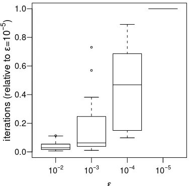
The main parameter that influences the hybrid algorithm is the stopping crite-rion ǫ. The algorithm switches from the EM to the Newton-type algorithm as soon as the relative change in the log-likelihood of two subsequent steps falls below a predefined value ǫ.
[image:40.595.184.372.508.693.2]Different choices of the stopping criterionǫhave mainly two effects. Firstly, on the one hand, a small ǫ in general leads to a low failure rate of the algorithm (i.e., cases in which no maximum of the log-likelihood is found) and a high proportion of successful convergence to the global maximum. Secondly, on the other hand, small values of ǫincrease the computational time required by the algorithm. Figure 3.2 shows boxplots of the number of EM iterations of the hybrid algorithm for different values ofǫ, relative to the numbers of iterations obtained for the smallest value studied, i.e. ǫ= 10−5.
Figure 3.2: Effect of the stopping criterion ǫ in the hybrid algorithm on the number of EM iterations, relative to ǫ= 10−5
ε
iterations (relative to
ε
=
10
−
5 )
10−2 10−3 10−4 10−5
The relative number of EM iterations increases moderately when using ǫ = 10−3 instead of ǫ = 10−2, while it rises substantially when moving down to
ǫ= 10−4 orǫ = 10−5. Since the proportion of successful estimations improves
only slightly for smaller values of ǫ, the choice of ǫ = 10−3 is a reasonable
compromise to deal with the trade-off between speed and stability and is used in what follows.
Fitting HMMs to the 24 time series with the same combinations of initial values mentioned above leads to the results displayed in Table 3.2, which clearly shows the high stability of the hybrid algorithm. The EM algorithm as well as the hybrid algorithm provide the most stable results (with their order changing from series to series). Not surprisingly, the Nelder-Mead algorithm is more stable than the Newton-type algorithm. However, there may be cases in which both the EM and the hybrid algorithm provide just a slight improvement over direct numerical maximization. It should also be mentioned that, as in the study of the parameterizations for direct numerical maximization, the results depend on the true parameters that were used to generate the observations. The results concerning the dependence of the stability on the true parameter settings described above also hold for the EM and the hybrid algorithm.
Table 3.2: Performance of the algorithms considered
failures (%) global maximum found (%)
Newton-type 0.17 84.3
Nelder-Mead 0.00 93.0
EM algorithm 0.00 95.6
Hybrid algorithm 0.00 95.4
The robustness of the EM and the hybrid algorithm is illustrated in Figure 3.3. The design of the figure corresponds to the design of Figure 3.1. It shows the proportion of successful estimations for specific combinations of the initial values for the state-dependent parameters, λs
0, λs1, or the diagonal elements of
the initial TPM,ps
00, ps11. The algorithms for parameter estimation are applied
for the same series as above.
Figure 3.3: Proportion of successful estimations for specific combinations of the parameter starting values using different algorithms for parameter estimation
0 1 2 3 4 5 6 0 1 2 3 4 5 6
λ0s λ1
s
Newton−type algorithm
0 1 2 3 4 5 6 0 1 2 3 4 5 6
λ0s λ1
s
Nelder−Mead algorithm
0 1 2 3 4 5 6 0 1 2 3 4 5 6
λ0s λ1
s
EM algorithm
0 1 2 3 4 5 6 0 1 2 3 4 5 6
λ0s λ1
s
Hybrid algorithm
0.0 0.2 0.4 0.6 0.8 1.0 0.0 0.2 0.4 0.6 0.8 1.0
p00s
p11
s
0.0 0.2 0.4 0.6 0.8 1.0 0.0 0.2 0.4 0.6 0.8 1.0
p00s
p11
s
0.0 0.2 0.4 0.6 0.8 1.0 0.0 0.2 0.4 0.6 0.8 1.0
p00s
p11
s
0.0 0.2 0.4 0.6 0.8 1.0 0.0 0.2 0.4 0.6 0.8 1.0
p00s
3.2.4
Coverage probability of confidence intervals
In this section we consider the estimation of confidence intervals for the pa-rameters of HMMs and their properties. These may also be calculated based on the asymptotic properties of the estimators, but we will restrict our atten-tion to those based on the parametric bootstrap as described, for example, in MacDonald & Zucchini (1997).
Bootstrap confidence intervals for the parameters of a HMM have already been studied by Visser et al. (2000), but we could find no detailed analysis of the true coverage probability of bootstrap confidence intervals in the context of HMMs.
We therefore apply a double parametric bootstrap method to analyze the cov-erage probability of bootstrap percentile confidence intervals (Efron & Tibshi-rani 1993, Chapter 13) using the hybrid algorithm introduced above, and at different levels of confidence (90%, 95% and 99%).
In a first step, for each of the 24 true parameter combinations listed in Sec-tion 3.2.1, we generated 1000 realizaSec-tions of the respective Poisson HMM. In a second step, we computed the maximum likelihood estimates for these 1000 realizations and, in each case, simulated 200 new bootstrap realizations using the obtained parameter estimates. We then constructed confidence intervals applying the bootstrap percentile method to the new bootstrap samples, us-ing different levels of confidence. Thus we obtained 1000 confidence intervals for each of the true parameters of the respective HMMs, and at each level of confidence. The coverage probabilities were then estimated as the proportion of those confidence intervals that cover the respective true parameter value.
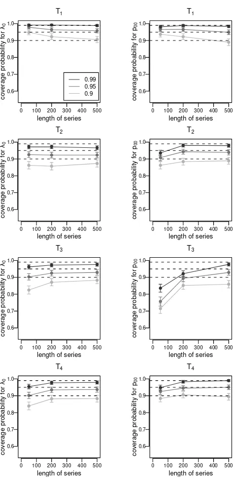
The resulting coverage probabilities (and the respective confidence intervals) for the parametersλ0andp00, for three different levels of confidence, depending
on the length of the time series and the true TPM, are given in Figure 3.4 for a true state-dependent parameter vector λ with a relatively large difference between the state-dependent values λi, and in Figure 3.5 for a true λ vector
Figure 3.4: Coverage probabilities of bootstrap confidence intervals with dif-ferent levels of confidence for series simulated using λ2, i.e. a large difference
between the state-dependent parameters
0 100 200 300 400 500 0.6
0.7 0.8 0.9 1.0
length of series
coverage probability for
λ0
T1
0.99 0.95 0.9
0 100 200 300 400 500 0.6
0.7 0.8 0.9 1.0
length of series
coverage probability for
p00
T1
0 100 200 300 400 500 0.6
0.7 0.8 0.9 1.0
length of series
coverage probability for
λ0
T2
0 100 200 300 400 500 0.6
0.7 0.8 0.9 1.0
length of series
coverage probability for
p0
0
T2
0 100 200 300 400 500 0.6
0.7 0.8 0.9 1.0
length of series
coverage probability for
λ0
T3
0 100 200 300 400 500 0.6
0.7 0.8 0.9 1.0
length of series
coverage probability for
p00
T3
0 100 200 300 400 500 0.6
0.7 0.8 0.9 1.0
length of series
coverage probability for
λ0
T4
0 100 200 300 400 500 0.6
0.7 0.8 0.9 1.0
length of series
coverage probability for
p0
0
Figure 3.5: Coverage probabilities of bootstrap confidence intervals with dif-ferent levels of confidence for series simulated using λ1, i.e. a small difference
between the state-dependent parameters
0 100 200 300 400 500 0.6
0.7 0.8 0.9 1.0
length of series
coverage probability for
λ0
T1
0.99 0.95 0.9
0 100 200 300 400 500 0.6
0.7 0.8 0.9 1.0
length of series
coverage probability for
p00
T1
0 100 200 300 400 500 0.6
0.7 0.8 0.9 1.0
length of series
coverage probability for
λ0
T2
0 100 200 300 400 500 0.6
0.7 0.8 0.9 1.0
length of series
coverage probability for
p0
0
T2
0 100 200 300 400 500 0.6
0.7 0.8 0.9 1.0
length of series
coverage probability for
λ0
T3
0 100 200 300 400 500 0.6
0.7 0.8 0.9 1.0
length of series
coverage probability for
p00
T3
0 100 200 300 400 500 0.6
0.7 0.8 0.9 1.0
length of series
coverage probability for
λ0
T4
0 100 200 300 400 500 0.6
0.7 0.8 0.9 1.0
length of series
coverage probability for
p0
0
It is observed that in most cases for τ = 50 the true coverage probability deviates from the desired level of confidence. On the other hand, in the case of a relatively large difference between the true λi-values, the true coverage
probabilities of the confidence intervals nearly correspond to the desired levels of confidence for series of length τ = 200 or τ = 500. The influence of the transition probability matrix on the coverage probability also becomes obvious. Especially in the case of the true TPM T3, which represents a HMM in which
the states switch frequently, the coverage probability of the confidence interval for p00 deviates substantially from the nominal coverage probability even for
τ = 200.
In contrast, in the case where the λi-values differ less from each other, all
coverage probabilities, except those for the transition probability matrix T1 (a case in which the states are highly persistent) are clearly smaller than the nominal level. This holds true even for relatively long time series of τ = 500, indicating that the estimated confidence intervals are too narrow. Similar results hold for the other parameters, which are not shown in the figures. These results coincide with the findings of Nityasuddhi & B¨ohning (2003), who investigated normal mixtures and reported that the asymptotic properties of the EM algorithm are inaccurate when the means lie close to each other.
3.3
An application
In this section we report on the performance of the hybrid algorithm when this is applied to a set of real data. The time series consists of yearly counts of major world earthquakes, i.e. earthquakes of magnitude 7.0 or greater on the Richter scale, between the years 1900 to 20033.
This series has already been studied by Zucchini & MacDonald (1998), however with restriction to the period 1900-1997. Since these authors select the three-state HMM as the best model we restrict our attention here to the case of a three-state Poisson HMM.
We use an estimation grid similar to the one used in the previous section. The initial values λs
0, λs1, λs2 for the grid search are chosen from 10 equidistant
points in [xmin, xmax], whereλs0 < λs1 < λs2, and the starting values of the TPM
are given by ps
ii ∈ {0.2,0.4,0.6,0.8} for i = 0,1,2 and pijs = (1−psii)/2 for
i= 0,1,2, j 6=i, yielding a total of 7680 grid points.
3
The ML estimates obtained for the earthquakes series are ˆλ= (11.4,19.1,29.4) and
ˆ T =
00..855 0055 0..121 0895 0..024050 0.000 0.194 0.806
leading to logLmax = −324.79. These results are close to the ones given by
Zucchini & MacDonald (1998).
[image:47.595.231.409.553.707.2]Figure 3.3 provides boxplots of the computational time needed when using a Newton-type algorithm, the EM algorithm and the hybrid algorithm. Since computational time depends on both the hardware and software used, the computational times in Figure 3.3 are normalized by the average computational time needed by the fastest method, the Newton-type algorithm as implemented in the R function nlm(). Thus the mean computational time is 1.00 for the Newton-type algorithm, 1.84 for the EM and 1.44 for the hybrid algorithm. All three algorithms considered never failed to provide a result, though the Newton-type algorithm succeeded only in 66.7% to attain the global maximum of the likelihood, while the EM and the hybrid algorithm led to the global maximum in 100% and 98.7% of all grid search trials, respectively. Hence, it is observed that the hybrid algorithm provides a reasonably efficient method to increase the stability when compared to the Newton-type algorithm and the speed when compared to the EM algorithm.
Figure 3.6: Scaled computational time and percentage of trials with conver-gence to the global maximum using different algorithms for parameter estima-tion of the quakes series
EM Newton−type Hybrid 0.2
0.5 1.0 2.0 5.0 10.0 20.0
scaled computational time
Global maximum found
In this application, the reduction of computational time when using the hybrid algorithm instead of the EM algorithm seems to be relatively small. However, in the simulation experiment described above we found series of lengthτ = 200 or τ = 500 for which the mean computational time of hybrid algorithm could be reduced substantially compared to that of the EM algorithm.
3.4
Conclusion
We presented different methods of parameter estimation for HMMs, among others an EM algorithm for stationary time series. In the cases investigated here, it turned out that the simplest parameterization for the direct numerical maximization provides the best results. Comparison of the EM algorithm and direct numerical maximization clearly showed the trade-off between stability and performance. The hybrid algorithm would seem to provide an excellent compromise, because it is not only as stable as the EM-algorithm, but also clearly faster. If a choice has to be made between the EM algorithm and DNM, the latter is preferable if one can provide accurate initial values, or if the estimation is time-critical. Clearly, if the formulae required for the EM algorithm are too difficult to derive, or if one wishes to avoid deriving these, then one has to use DNM. In all other situations, the EM algorithm is the preferred method due to its greater stability.
We also found that the true coverage probability for bootstrap-based confi-dence intervals, obtained by parametric bootstrap, can be unreliable for models whose state-dependent parameters lie close to each other.
Our analysis can easily be extended to cover other component distributions. A smaller investigation of Normal HMMs revealed tendencies similar to those obtained for the Poisson HMMs, although the results were not as clear-cut. A complicating factor in the important special case of Normal HMMs is that each state-dependent distribution depends on two parameters and, further-more, the likelihood function is – as for independent normal mixtures – in fact unbounded (Nityasuddhi & B¨ohning 2003).
Markov Switching Approaches
to Model Time-Varying Betas
Modeling daily return series with HMMs has been investigated by several au-thors. After the seminal work of Ryd´en et al. (1998) who showed that two-and three-state HMMs with normal components reproduce well the temporal and distributional properties of daily returns from the S&P 500 index, several other authors followed their ideas (see, e.g., Cecchetti et al. 1990, Linne 2002, Bialkowski 2003).
The focus of this chapter lies on the development of a joint model for return series. Consider a portfolio consisting of multiple assets, e.g., a portfolio of European shares selected from the Dow Jones (DJ) EURO STOXX 600. Fit-ting a multivariate HMM with normal component distributions would require the estimation of the variance-covariance matrix for each of the states. In the worst case, the portfolio of a professional investor is composed of all 600 shares and thus the procedure would involve a matrix of dimension 600×600 yielding 180300 parameters to be estimated per state. It is obvious that such a model would be grossly over-parameterized resulting in very unstable esti-mates. Moreover, as shown in Chapter 3, the common estimation algorithms for HMMs depend on the choice of the initial values. Hence, choosing even a small number of different initial values for each parameter may yield an infea-sible amount of estimations to be carried out.
A possible solution to the quadratic increase of the number of parameters is based on the Capital Asset Pricing Model (CAPM). In the CAPM, the return of every single asset is linearly dependent to the market return (plus an error term):