Munich Personal RePEc Archive
Projecting Progress toward the
Millennium Development Goals
White, Howard and Blondal, Nina
Institute of Development Studies, University of Sussex
August 2007
Copyright © UNU-WIDER 2007 *IDS, University of Sussex
This study has been prepared within the UNU-WIDER project on the Millennium Development Goals: Assessing and Forecasting Progress, directed by Mark McGillivray.
UNU-WIDER acknowledges the financial contributions to the research programme by the governments of Denmark (Royal Ministry of Foreign Affairs), Finland (Ministry for Foreign Affairs), Norway (Royal Ministry of Foreign Affairs), Sweden (Swedish International Development Cooperation Agency—Sida) and the United Kingdom (Department for International Development).
ISSN 1810-2611 ISBN 92-9190-990-4 ISBN 13 978-92-9190-990-2
Research Paper No. 2007/47
Projecting Progress toward the
Millennium Development Goals
Howard White and Nina Blöndal
*August 2007
Abstract
The Millennium Development Goals have become the frame of reference for most of the development community: the standard by which performance will ultimately be judged. Given their importance, considerable attention has been paid as to whether these goals will be met or not. The overwhelming conclusions from such analyses are not positive. The goals will not be met. There are exceptions—education has expanded rapidly, although questions are raised about quality, and some countries, notably in South East Asia, but also South Asia to a lesser extent, have done well across the board and will meet several of the goals. But many countries, most especially in Africa, will not. The projections show that poverty will become more heavily concentrated in Africa in both relative and absolute terms. In addition, whilst urban poverty will increase, in 2015 poverty will remain a predominately rural phenomenon, with 60-70 per cent of the poor (depending on the measure) living in rural areas. But these projections are based on assumptions, including the assumption of business as usual. Various adverse shocks may result in far worse scenarios. On the other hand, more intensive promotion of pro-poor policies can mean that the goals might yet be realized.
Keywords: Millennium Development Goals, poverty projections, mortality, nutrition, poverty, education, health, inequality
The World Institute for Development Economics Research (WIDER) was established by the United Nations University (UNU) as its first research and training centre and started work in Helsinki, Finland in 1985. The Institute undertakes applied research and policy analysis on structural changes affecting the developing and transitional economies, provides a forum for the advocacy of policies leading to robust, equitable and environmentally sustainable growth, and promotes capacity strengthening and training in the field of economic and social policy making. Work is carried out by staff researchers and visiting scholars in Helsinki and through networks of collaborating scholars and institutions around the world.
www.wider.unu.edu [email protected]
UNU World Institute for Development Economics Research (UNU-WIDER) Katajanokanlaituri 6 B, 00160 Helsinki, Finland
Typescript prepared by Lorraine Telfer-Taivainen at UNU-WIDER
The views expressed in this publication are those of the author(s). Publication does not imply endorsement by the Institute or the United Nations University, nor by the programme/project sponsors, of any of the views expressed.
Acknowledgements
1 Introduction
Since the adoption of the International Development Targets, and their successor Millennium Development Goals (MDGs), a growing number of publications have presented estimates of development outcomes in 2015, the target year for most of the goals. What most these projections show is that the developing world as a whole is ‘off track’ with respect to most targets. They will not, in aggregate, be met and many countries will fall far short. The MDGs seem set to pass into history as another set of missed development targets.
This paper looks at the soundness of these dire projections. Section 2 briefly discusses the basis for making such projections and then findings for major MDG targets (income poverty, mortality, education, nutrition and HIV/AIDS in Sections 3-7). Section 8 concludes.
2 Approaches to making projections1
Projections may vary because of differences in assumptions regarding (1) determinants of the outcome of interest, (2) model parameters, or (3) future values of the determinants. The simplest models, and by far the most common approach, take time as the only determinant, i.e., the future is forecast-based on historical trends, an approach called here naïve projections. Naïve projections tell us if a country is on track or not to meet the relevant goal, which is certainly of policy interest, but are of less use in predicting actual expected values at some point in the future unless its determinants really are uncertain or unforecastable.
The next most common approach is to use an outcome-income elasticity to base the forecast on projections of economic growth, the latter usually being taken from some other source, such as the World Bank’s Global Economic Prospects (GEP). Since income is highly correlated with most of the outcomes of interest, this approach can be expected to give a reasonable first approximation. However the correlation with income is imperfect, so adding more variables to the right-hand side of the determinants-equation will help, at least if the future values of these determinants can be predicted with any degree of confidence. More sophisticated versions utilize multi-equation models. There are undoubted advantages to such models, which allow a wider range of policy simulations, but they are quite resource intensive and assumption dependent. Results from the most recent multi-equation model, the World Bank Maquette for MDG Simulations (MAMS), are thus far only available for one country (Ethiopia), and such approaches are not the basis of the projections presented here.
Some indicators have risen in recent years at a far greater rate than their historical precedent—primary enrolment being the most obvious case. In these cases, if naïve projections are based on very recent trends then such forecasts may be superior to those which are model-based. But naïve projections will under-estimate future growth if the period used to calculate expected growth includes many years prior to any recent expansion. The main point is that policy can make a difference to the achievement of
goals—as shown by the experience of countries which do not follow the expected outcome-income trajectory (see World Bank 2005, for a discussion of Bangladesh which has been remarkably successful in reducing fertility and mortality faster than growth would suggest). If the right policies were to be implemented, then all future outcomes would be better than suggested here, though this of course begs the question as to what the ‘right policies’ are.
A further source in variation of projections is the level of disaggregation at which they are made. Although most sources report results at the regional level, it is preferable that these regional aggregates be based on country-level projections using country-specific data and parameters. This is not always the case. All methods are of course dependent on the quality of data used. Data availability has improved greatly in the last two decades, though most outcomes are not available on an annual basis.2 There are also exceptions to the general increase in data availability, such as maternal mortality and literacy, for which data are less reliable. Moreover, even where data are good there are frequently groups missed from the data, notably those not in fixed households (nomads, street children, those in institutions, etc.).
Basis of own projections
Our own projections are made at the country level and are reported using either the UN or World Bank regional classifications. The baseline data (i.e. pre-projection) are from the UN Millennium Indicators Database, supplemented by the World Bank’s World Development Indicators and Demographic and Health Survey (DHS) data as necessary. Population data are from the UN Population Database 2004 Revision. Projections are made using one of three methods: (1) naïve projections, (2) growth-based estimates, and (3) model-based estimates (i.e. growth plus other factors). The latter two approaches use differential elasticities to capture the greater poverty-reducing effect of growth in low inequality settings. Rural-urban rates are based on country-specific estimates of the rural-urban differential. Specific details of the projections are as follows:
• Income poverty is modelled as a function of income growth alone with the elasticity varying according the level of initial inequality.
• Under-five mortality is modelled as a function of income poverty (elasticity = 0.4) and female enrolments (elasticity = -1.3) and an autonomous decline of 1.5 per cent per annum.
• Under-nutrition is modelled as a function of income alone, with the elasticity again varying by the level of inequality.
• Net enrolments are based on naïve projections, made separately for male and female, capped at 98 and the female rate capped at the male rate.
• Literacy is calculated in two ways: (1) naïve projections, done separately for male and female, and capped at 99.5, and (2) an accounting approach based on age structure and net enrolments, removing older, less literate, people from the population and adding those graduating from school who are assumed to be literate. Again the data are capped at 99.5.
• Separate rural and urban estimates are made by using the ratio of rural to urban incidence, based on observed values where available and modelled (as a function of poverty, urbanization, education and regional dummies) when not available.
3 Income poverty
Early estimates of progress toward reducing income poverty come from studies conducted by the Institute of Social Studies for the Sida 2015 project (hereinafter the ISS study, Hanmer et al. 1997a, 1997b), and work undertaken by the Overseas Development Institute (ODI).3 These two studies made forecasts based on estimates of the elasticity of poverty with respect to income, allowing the elasticity to vary according to the degree of inequality.4 The World Bank has since begun publishing annual estimates of income poverty in 2015 in Global Economic Prospects (GEP). These estimates are the same as those to be found in the Bank’s MDG Global Monitoring
Report. The methodology used in these studies is not public, but appears to be based on
household data rather than cross-country elasticities. Elasticities based on household data are generally higher than those from cross-country regressions, so the estimates of future numbers of poor will be less than if elasticities estimated using cross-country data are used.
Our own estimates follow the ODI-Sida approach applied on a country-by-country basis. Projected growth rates are based on regional averages from GEP, with a few exceptions. The poverty elasticity is assumed to vary according to initial inequality.5 To calculate regional figures of absolute numbers of poor, the total for the region is scaled-up to capture the population not covered by the data.
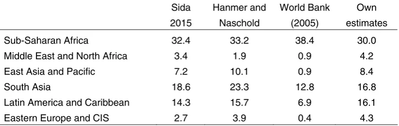
Table 1 summarizes the various results. The most recent World Bank estimates present a more positive picture than do the earlier studies, except with respect to sub-Saharan Africa (SSA). Our own estimates give figures more similar to those of the earlier studies. In general this will be because we assume lower elasticities than those used by the World Bank, especially for high inequality countries, so the rate of poverty reduction as a consequence of growth is less. However, in the case of Africa, our estimates are more positive. This discrepancy is most likely as the World Bank is using recent country-specific poverty estimates not available to us. Discrepancies also arise from both differing assumed growth rates and data revisions to poverty estimates in the base year (1990). More recent growth forecasts are generally more positive than the older ones6 and estimates of poverty in 1990 have been revised downward, especially for Latin America and the Caribbean (LAC).
3 The same person, Lucia Hanmer, was responsible for the design of the quantitative aspects of both these studies.
4 Forecasting was also carried out by Demery and Walton (1998) from the World Bank using an approach similar to that used in the ISS and ODI studies, though the results were not presented in a way allowing regional tabulations.
5 The elasticity is taken as -0.5, -0.8 and -1.2 for high, middle and low inequality countries respectively, where the former has a Gini coefficient of ≥ 0.54 and the latter ≤ 0.40.
Table 1: Income poverty forecasts (% living below $1 a day) for 2015 from three studies Sida 2015 Hanmer and Naschold World Bank (2005) Own estimates
Sub-Saharan Africa 32.4 33.2 38.4 30.0
Middle East and North Africa 3.4 1.9 0.9 4.2
East Asia and Pacific 7.2 10.1 0.9 8.4
South Asia 18.6 23.3 12.8 16.8
Latin America and Caribbean 14.3 15.7 6.9 16.1
Eastern Europe and CIS 2.7 3.9 0.4 4.3
Source: See text.
Income poverty will be increasingly concentrated in Africa (Figure 1), with absolute numbers of poor under the $1 a day standard in Africa overtaking South Asia at around the current time. If a $2 a day poverty line is used then South Asia will continue to have the bulk of the world’s income poor in 2015 (46 per cent), followed by SSA (31 per cent).
Figure 1: Share of global poverty (proportion of poor in each region using $1 a day poverty line) 0 10 20 30 40 50 60 East Asia and Pacific Europe and Central Asia Latin America and Caribbean Middle East and North Africa
South Asia Sub-Saharan Africa S ha re of gl oba l pov e rt y ( % )
1990 2001 2015
Source: Calculated from World Bank GEP data.
Sub-regional estimates
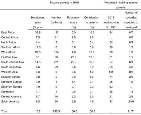
[image:7.595.74.438.371.589.2]Table 2: Sub-regional income poverty estimates 2015 ($1 a day)
Income poverty in 2015 Progress in halving income poverty
Headcount ratio (% poor)
Number (millions)
Population share
(%)
Contribution to poverty
(%)
2015 headcount as
% 19901
Number of countries expected to
meet goal2
East Africa 33.8 122 5.0 16.6 84 0/7 Central Africa 7.5 11 2.0 1.5 .. 0/0
North Africa 1.4 3 3.1 0.4 64 0/3
Southern Africa 11.3 6 0.8 0.8 89 1/5
West Africa 37.5 124 4.6 16.8 78 1/9 Eastern Asia 6.1 98 22.2 13.3 21 1/1 South-central Asia 14.5 271 25.8 36.8 37 6/9 South-east Asia 4.6 29 8.6 3.9 29 4/6
Western Asia 3.3 9 3.6 1.2 141 0/2
Eastern Europe 3.0 9 3.9 1.2 74 2/9
Northern Europe 1.0 1 1.4 0.1 25 1/2
Southern Europe 1.0 2 2.1 0.2 52 ..
Caribbean 1.7 1 0.6 0.1 55 1/3
Central America 9.7 16 2.3 2.2 51 2/5
South America 8.5 36 5.9 4.9 97 2/10
Total 10.2 736.3 100.0 100.0 .. 21/71
Notes: (1) calculated using only countries for which estimates available for both 1990 and 2015. (2) second figure is the number of countries for which early 1990s income poverty data were available. (Data availability for this column is less than that used for poverty projections, as more recent poverty data were usually used for the projections.)
Source: Authors’ estimates.
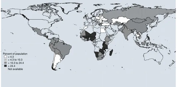
Figure 2: Income poverty 2015 (growth-based projections, differential elasticities)
Percent of population < 4.3
Rural versus urban poverty
[image:10.595.94.527.344.524.2]The poverty rate is generally higher in rural areas than urban. Data were available on rural and urban poverty rates using the national poverty line for 56 countries for various years in the 1990s. The mean ratio of numbers of rural and urban poor was 1.86 (and the median 1.53). For only seven of the 56 countries was urban poverty higher than rural, compared to 18 in which it was over twice as high in rural areas. In order to generate urban and rural poverty estimates for a larger number of countries this ratio was imputed based on a regression of determinants.7 The estimates are made at the country level, using (1) mostly regional growth rates with some country-specific adjustments, and (2) elasticities which vary according to the degree of initial inequality. The main finding is that in 2015 two-thirds of the world’s income poor will be in rural areas. The majority of the populations in Africa and Asia will be rural until after 2020. Given the higher poverty rate in rural areas (16 per cent globally compared to 7 per cent in urban areas), it follows that these areas must account for a disproportionate number of the poor (Table 3).
Table 3: Rural and urban poverty in 2015: headcount ratio and millions of people ($1 a day)
Headcount ratio Millions of people
Total Urban Rural Total Urban Rural
Per
cent
rural
Sub-Saharan Africa 30.0 21.6 37.4 282 86 196 69.6
Middle East and North Africa 2.8 1.6 4.2 10 4 6 63.6
E. Europe and Central Asia 3.2 2.5 4.3 15 8 7 47.9
East Asia and Pacific 5.7 3.1 8.4 120 33 87 72.5 South Asia 14.8 10.6 16.8 255 59 196 76.8
L. America and Caribbean 8.7 7.0 16.1 54 35 19 35.3
Total 11.8 7.4 16.3 737 225 512 69.5
Source: Authors’ estimates (see Appendix).
Summary
Recent estimates show that Africa is overtaking South Asia as the region with the largest number of those living on less than a dollar a day, and by 2015 half of those below this poverty line globally will be in that region. The prospects for most of Africa meeting the MDG of halving income poverty seem remote. These trends reflect both the region’s poorer growth performance and the fact that it has high and growing levels of inequality. By contrast the share of East Asia in world poverty is falling rapidly and will be only 3 per cent by 2015; this region will meet the MDG as will other parts of Asia. Latin American countries will be close to achieving the goal, but excluding several in South America. If a higher poverty line of $2 a day is used then the global poverty profile shifts, with South Asia again having most the world’s
poor, followed by Africa. Income poverty is higher in rural areas than urban ones. In 2015, 70 per cent of the income poor will live in rural areas.
4 Mortality
Different estimates
[image:11.595.91.534.393.671.2]Hanmer and Naschold (2000) provide regression-based estimates of infant and under-five mortality allowing for income, HIV/AIDS, education and health services.8 However, there have been substantial upward revisions to mortality estimates in the base year (1990) since they carried out their analysis, so it is to be expected that their results have a downward bias. Indeed, the figures are lower than those available from other sources. Using data from the World Bank Global Monitoring Report, we made our own naïve projections at the regional level, and then adjusted these to allow for expected higher future growth. We also made country-specific estimates using a model based on poverty levels and female primary enrolment. The final estimates are those from the UN World Population Prospects, 2004 revision. These estimates are based on demographic trends, without reference to economic conditions, but nonetheless appear broadly consistent with the growth-adjusted estimates we made.
Table 4: Mortality estimates 2015 (rates per 1,000)
Own projections
Hanmer
and
Naschold
Naïve
projection
Growth
adjusted
Model
based
UN
population
projections
Under-five mortality
Sub-Saharan Africa 118 168 138 97 130
Middle East and North Africa 34 42 30 31 28
East Asia and Pacific 8 30 32 27 30
South Asia 55 78 75 50 69
Latin America and Caribbean 15 25 10 24 22
Eastern Europe and Central Asia 6 29 30 25 30
Infant mortality
Sub-Saharan Africa 67 96 89 89 80
Middle East and North Africa 22 53 28 28 25
East Asia and Pacific 7 24 27 27 25
South Asia 43 54 56 56 51
Latin America and Caribbean 14 19 29 29 17
Eastern Europe and Central Asia 10 25 31 31 6
Note: Own projections are at regional level for model-based. Source: See text.
However, the model based estimates show a stronger reduction in mortality, notably in SSA and South Asia, this discrepancy being driven by rapid growth of female enrolments in some countries and the fact that the model does not allow for additional AIDS related deaths (Table 4).
Sub-regional and country data
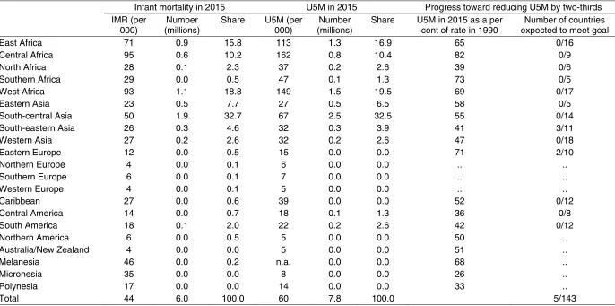
Table 5 shows the sub-regional figures using the UN Population projection estimates. Rates are highest in West and Central Africa. These are both areas in which tropical diseases remain important and so have unusually high ratios of child to infant deaths. But they are also areas in which conflict has adversely affected mortality. The maps show the scar of premature death running across Africa (Figure 3).
Some trends
Table 5: Sub-regional estimates of infant and under-five mortality, 2015
Infant mortality in 2015 U5M in 2015 Progress toward reducing U5M by two-thirds IMR (per
000)
Number (millions)
Share U5M (per 000)
Number (millions)
Share U5M in 2015 as a per cent of rate in 1990
Number of countries expected to meet goal East Africa 71 0.9 15.8 113 1.3 16.9 65 0/16 Central Africa 95 0.6 10.2 162 0.8 10.4 82 0/9
North Africa 28 0.1 2.3 37 0.2 2.6 39 0/6 Southern Africa 29 0.0 0.5 47 0.1 1.3 73 0/5 West Africa 93 1.1 18.8 149 1.5 19.5 69 0/17 Eastern Asia 23 0.5 7.7 27 0.5 6.5 58 0/5 South-central Asia 50 1.9 32.7 67 2.5 32.5 55 0/14 South-eastern Asia 26 0.3 4.6 32 0.3 3.9 41 3/11 Western Asia 27 0.2 2.6 32 0.2 2.6 47 0/18 Eastern Europe 12 0.0 0.5 15 0.0 0.0 71 2/10 Northern Europe 4 0.0 0.1 6 0.0 0.0 .. .. Southern Europe 6 0.0 0.1 7 0.0 0.0 .. .. Western Europe 4 0.0 0.1 5 0.0 0.0 .. ..
Caribbean 27 0.0 0.6 39 0.0 0.0 52 0/12 Central America 14 0.0 0.7 18 0.1 1.3 36 0/8
South America 18 0.1 2.0 22 0.2 2.6 42 0/12 Northern America 6 0.0 0.5 5 0.0 0.0 50 .. Australia/New Zealand 4 0.0 0.0 5 0.0 0.0 51 ..
Melanesia 46 0.0 0.2 n.a. 0.0 0.0 68 ..
Micronesia 35 0.0 0.0 8 0.0 0.0 26 ..
Polynesia 17 0.0 0.0 14 0.0 0.0 33 ..
Total 44 6.0 100.0 60 7.8 100.0 5/143
Figure 3: Under-five mortality 2015 (UN Population Projection, 2004 Revision)
Deaths per 1,000 live births
However, as with income poverty reduction, the rate of decline is rarely sufficient to meet the ambitious goal of a two-thirds reduction by 2015. Our own projections suggest that only five countries will do so: Indonesia and Vietnam are the only two of significance (the others are Montserrat and Vanuatu; outside the sample, Portugal, Moldova and the Czech Republic will also do so). The UN Population projections are more optimistic, showing 10 countries expected to reach the target, with Egypt, Syria and Tunisia being amongst those added to the list.
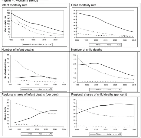
Figure 4: Mortality trends
Infant mortality rate Child mortality rate
0 20 40 60 80 100 120 140 160 180 200
1950 1970 1990 2010 2030
In fa n t m o rt a li ty r a te
Africa Asia LAC
0 10 20 30 40 50 60 70 80 90
1985 1995 2005 2015 2025 2035 2045
Africa Asia LAC
Number of infant deaths Number of child deaths
0 2 4 6 8 10 12 14
1940 1960 1980 2000 2020 2040 2060
N o . o f d e a th s ( m illio n s )
Africa Asia LAC
0.0 0.5 1.0 1.5 2.0 2.5 3.0
1985 1995 2005 2015 2025 2035 2045
Africa Asia LAC
Regional shares of infant deaths (per cent) Regional shares of child deaths (per cent)
0 10 20 30 40 50 60 70 80 90
1940 1960 1980 2000 2020 2040 2060
S h ar e o f d eath s
Africa Asia LAC
0 10 20 30 40 50 60 70 80
1985 1995 2005 2015 2025 2035 2045
Africa Asia LAC
Source: Based on UN Population Projections 2004 revision
Rural and urban differences
was over two in the case of Peru. The contrast is stronger for child mortality, with the average ratio being 1.7 (median 1.6), in only five cases was rural mortality lower than that in urban areas, and rural mortality was double that in urban areas in 30 cases, reaching a ratio of 4.9 in Armenia. There are no clear regional patterns in these differentials. For simulation purposes, actual values of the ratio for under-five mortality are used for those countries covered by the survey, with remaining countries set at the sample median (1.4).9 The results are shown in Table 6 (applied to the model-based estimates). Of the 30 million under-five deaths in 2015, 20 million (i.e. two-thirds) will take place in rural areas.
Table 6: Rural urban differentials in under-five mortality, 2015
U5M rate (per 000) Number (millions)
Urban Rural Total Urban Rural Total
Sub-Saharan Africa 81 108 97 4.9 9.2 14.1 Middle East and North Africa 24 39 31 0.6 0.6 1.2 Europe and Central Asia 21 32 25 0.4 0.3 0.7 East Asia and Pacific 19 35 27 1.4 2.5 3.9
South Asia 36 57 50 2.0 6.7 8.7
Latin America and Caribbean 22 36 24 0.9 0.4 1.3
Total 37 63 51 10.3 19.8 30.0
Source: Authors’ estimates.
Water supply
Lack of access to water will be a largely rural phenomenon by 2015: three quarters of the 761 million without access to water will be in rural areas. Lack of access will be concentrated in East Asia and SSA which will together account for 80 per cent of those without access (Table 7).
Table 7: Access to water in 2015
Access to water (% of population)
Number without access (millions)
Urban Rural Total Urban Rural Total Share of total number globally
Share of those without access in rural areas Sub-Saharan Africa 82.2 57.6 69.3 72 227 288 38 79 Middle East and N. Africa 96.0 79.4 89.7 9 30 37 5 80 Europe and Central Asia 99.4 83.2 94.1 2 28 29 4 98 East Asia and Pacific 86.3 78.2 85.4 147 225 308 41 73 South Asia 95.7 94.9 95.6 24 59 77 10 77 L. America and Caribbean 98.0 85.4 96.5 10 18 22 3 81
Total 91.4 81.5 87.8 264 586 761 100 77
Source: Authors’ calculations, naïve projections.
Summary
All three major developing country regions have seen declining mortality, though it has been more rapid in Asia and Latin America and the Caribbean (LAC) than in Africa. But only in rare cases has the rate of reduction been at the 1.6 per cent a year required to achieve the MDG of a two-thirds reduction by 2015. Indeed, the rate of reduction in Africa has been insufficient to keep up with population growth, so the number of deaths is continuing to climb. As a result, Africa’s share of under-five deaths will continue to grow. In the case of infant deaths this trend represents a dramatic reversal. In the 1960s three-quarters of all infant deaths were in Asia, but by 2015 Africa will account for the majority, as it has done for child deaths for some years now, with the highest rates in Western and Central Africa. Two-thirds of these deaths will be in the rural areas of Africa, which is a similar share of under-five deaths in rural areas across the world.
Similar patterns reveal themselves with respect to critical determinants of under-five mortality: access to water and immunization. For example, West and Central Africa are also the two sub-regions with the lowest access to water expected in 2015. Over three-quarters of those without water in 2015 will be in rural areas. Immunization coverage fell in some countries in the 1990s and there remain a significant minority of countries with unacceptably low coverage rates.
5 Education
[image:18.595.93.495.321.435.2]The Millennium Project Task Force on Education (MPTFE) is the only study to estimate primary net enrolment rates.10 Projections are made based on predictive power of the s-curve (i.e. that later enrolments are harder) and suggest that SSA will continue to lag behind other regions with an estimated enrolment rate just under 80 per cent. South Asia and Middle East and North Africa are also estimated to lie below 90 per cent whilst other regions are expected to lie within five per cent of universal enrolment. This ‘last five per cent’ is increasingly recognized as being ‘problem groups’ requiring different policies. Our own country-level naïve projections do not allow for this effect, which may explain the higher figures in South Asia and LAC. Naïve projections seem appropriate since the policy push behind primary enrolments has enabled increases over and above those expected by economic performance or other possible determinants. It is the possibility of such a push in Africa which explain the higher rates there estimated by MPTFE. However, India began a very recent push, not yet shown in the data and so not picked up by naïve projections (Table 8).
Table 8: Net primary enrolment rate, 2015 (proportion of age cohort enrolled)
MPTFE Own projections
Sub-Saharan Africa 79.6 73.9
South Asia 86.1 92.4
Middle East and North Africa 88.0 89.3
Latin America and Caribbean 95.6 98.0
Eastern Europe and Central Asia 96.3 91.3
East Asia and Pacific 97.0 90.8
Sources: MPTFE and own projections.
The sub regional breakdown shows the problem in Africa to be least in southern Africa (Table 9), which is confirmed partially by the map, but it is patchy owing to limited data (Figure 5). Defining universal primary enrolment as an NER of 98 per cent shows that the majority of countries appear on track to achieve this goal.
Table 9: Sub-regional primary enrolment rates (NER) and numbers out of school, 2015 (millions)
No. NER
No. of
countries
with UPE
by 2015 No. NER
No. of
countries
with UPE
by 2015
East Africa 13.9 76.5 9/17 S. Europe 0.3 96.3 5/10
Central Africa 5.6 77.3 7/9 W. Europe 0.2 98.0 ..
North Africa 4.2 84.8 6/7 Caribbean 0.1 98.0 11/13
Southern Africa 0.6 90.5 1/5 C. America 0.4 98.0 24/24
West Africa 15.4 70.8 12/18 South America 0.9 98.0 8/8
Eastern Asia 9.3 91.8 4/7 N. America 0.6 98.0 ..
South-central Asia 19.1 91.2 10/14 Australia/NZ 0.0 98.0 ..
South-eastern Asia 6.3 90.2 7/11 Melanesia 0.2 85.8 ..
Western Asia 2.0 93.6 13/18 Micronesia 0.0 98.0 ..
Eastern Europe 0.8 95.2 5/10 Polynesia 0.0 98.0 ..
Northern Europe 0.2 97.6 11/13 Total 80.0 89.1 182/230
Source: authors’ projections.
Figure 5: Net enrolment rates 2015 (naïve projections)
Percent < 65 > 65 to > 85 to > 95
Numbers out of school
[image:21.595.70.503.179.363.2]Breaking down our own projections we see that SSA will account for nearly half of all the 80 million children out of primary school by 2015 (Table 10), reflecting the lower enrolment rates across the sub continent (Figure 5).
Table 10: Numbers of children out of school 2015 (millions)
Boys Girls Total
Proportion
girls
Share of total
out of school
Sub-Saharan Africa 17.9 21.4 39.3 54.5 48.8
Middle East and North Africa 2.4 2.4 4.7 49.8 5.9
E. Europe and Central Asia 1.3 1.8 3.1 59.0 3.9
East Asia and Pacific 9.5 5.9 15.4 38.4 19.1
South Asia 6.8 8.5 15.3 55.7 19.0
Upper middle income 0.7 0.7 1.3 50.0 1.7
High income 0.7 0.7 1.4 50.0 1.7
Total 39.2 41.4 80.6 51.4 100.0
Source: Authors’ projections.
Gender dimension
[image:21.595.72.497.511.650.2]Areas with low enrolments have a disproportionate number of girls out of school (see table above). The MPTFE study also provides estimates of gender equality in primary education measured by female to male net primary enrolment. Sub-Saharan Africa is estimated to have the lowest ratio with 93 girls to 100 boys (Table 11).
Table 11: Gender equality in education, female/male ratio 2015
Region MPTF on education
(primary)
MPTF on gender
(primary, gross)
Own estimates
(primary)
South Asia 95.3 111.0 99.6 Sub-Saharan Africa 93.2 94.6 98.8
Latin America and 99.1 96.2 100.0
Europe and Central Asia 99.3 98.3 99.2
East Asia and Pacific 98.8 98.4 101.1
Middle East and North Africa 96.0 100.0 100.0
Sources: UN Millennium Project (2005b), and own estimates.
Literacy
based on the net enrolment rate.11 The two approaches are not entirely consistent, with naïve projections predicting lower literacy. This is because recent rapid increases in enrolments are not yet reflected in higher literacy, but the accounting approach picks up these increases. However, both methods find that the vast majority of illiterates in 2015 will be in South Asia, with the majority of the remainder in SSA (Table 12).
Table 12: Literacy in 2015 by region
Naïve projections Accounting based
Literacy
rate
No. of
illiterates
(millions)
Literacy
rate
No. of
illiterates
(millions)
Sub-Saharan Africa 81.7 99 93.7 34
Middle East and North Africa 86.6 33 91.9 20
Europe and Central Asia 99.1 4 99.3 3
East Asia and Pacific 99.1 16 99.3 11
South Asia 68.1 387 80.9 232
Latin America and Caribbean 98.1 9 99.4 3
Developed 99.1 8 96.8 26
Total 89.6 555 93.8 329
Source: Authors’ calculations.
Summary
Sub-Saharan Africa will continue to lag behind other regions with respect to primary school enrolments with an estimated enrolment rate just under 80 per cent, though the problem is less in Southern Africa than elsewhere. South Asia and Middle East and North Africa are also estimated to lie below 90 per cent whilst other regions are expected to lie within five per cent from universal enrolment. However, this ‘last five per cent’ is increasingly recognized as being ‘problem groups’ requiring different policies.
6 Nutrition
Different estimates
Nutrition outcomes have been comprehensively modeled in three different sources: two IFPRI studies (Smith and Haddad 2000; von Braun et al. 2005) and FAO’s agricultural projections.12 In addition Onis et al. (2004) present sub-regional based naïve
11 Older people with lower literacy were removed from the population and younger people who have been to school added to it. It is being assumed that all those enrolled are literate on completion. This is certainly a rather heroic assumption, but it is one that already lays behind the literacy data themselves. Literacy is capped at 99.5 in all countries.
projections. The FAO study refers to adults who are undernourished (defined with reference to a calorie requirement of 1,900 kcal per day), whereas the IFPRI studies and Onis et al. refer to children only (using anthropometric measurement). The IFPRI results shown forecast for 2020 rather than 2015 (Table 13).
[image:23.595.71.450.265.637.2]The different estimates do not, in this case, give a similar picture. Smith and Haddad’s estimates are in general higher than those of Onis, and there is a marked discrepancy in the case of East Asia—which Smith and Haddad have as accounting for 15 per cent of children underweight by 2020, compared to Onis’ 3 per cent in 2015. Whilst, both have South Asia’s share as exceeding that of Africa, Smith and Haddad predict higher prevalence in South Asia than Africa, but Onis the reverse. FAO’s forecasts for adults give the two regions an equal share.
Table 13: Alternative estimates of underweight
Adults Children
FAO
(2015)
Smith and
Haddad (2020)
Onis et al.
(2015)
Prevalence
South Asia 12 37.4 26.2
Sub-Saharan Africa 23 28.8 29.2
East Asia 6 12.8 3.0
Near East and North Africa 7 5 7.4
Latin America and Caribbean 6 1.9 3.4
Numbers
South Asia 195 66 61.8
Sub-Saharan Africa 205 48.7 42.7
East Asia 135 21.4 3.0
Near East and North Africa 37 3.2 3.4
Latin America and Caribbean 40 1.1 2.0
Developing countries 612 140.4 112.9
Shares
South Asia 31.9 47.0 54.7
Sub-Saharan Africa 33.5 34.7 37.8
East Asia 22.1 15.2 2.7
Near East and North Africa 6.0 2.3 3.0
Latin America and Caribbean 6.5 0.8 1.8
Developing countries 100.0 100.0 100.0
Source: See text.
Some trends
[image:24.595.102.532.177.535.2]Figure 6 show trends from the FAO data. As mentioned above, the shares of Africa and Asia are about the same in 2015, reflecting a growing number of undernourished people in Africa, compared to a steady decline in South Asia.
Figure 6: Patterns and trends from FAO data
Prevalence of adult underweight, 2015 Share of adult underweight, 2015
0 5 10 15 20 25 Sub-Saharan Africa
Near East / North Africa
Latin America and
Caribbean
South Asia East Asia
P e rcen t u n d er w ei g h t 0 5 10 15 20 25 30 35 40 Sub-Saharan Africa
Near East / North Africa
Latin America and
Caribbean
South Asia East Asia
S ha re of unde rnut ri ti on
Prevalence of adult underweight, 1990-2030 Number of adult underweight, 1990-2030
0 5 10 15 20 25 30 35 40
1990/92 1997/99 2015 2030
P e rc e nt unde rw e ight
Sub-Saharan Africa North-East North Africa
LAC South Asia
East Asia 0 50 100 150 200 250 300 350
1990/92 1997/99 2015 2030
M il li ons un de rw e igh t
Sub-Saharan Africa North-East North Africa
LAC South Asia
East Asia
Source: FAO (2002).
Table 14: Per capita food consumption (calories per person per day)
1964-66 1997-99 2015
Developing countries 2054 2681 2850
Sub-Saharan Africa 2058 2195 2360
Near East/North Africa 2290 3006 3090
Latin America and the Caribbean 2393 2824 2980
South Asia 2017 2403 2700
East Asia 1957 2921 3060
Source: FAOSTAT (http://faostat.fao.org/).
Figure 7: Trends in agricultural output per person (2000=100)
0 20 40 60 80 100 120 140
1960 1970 1980 1990 2000
In
d
ex o
f ag
ri
cu
lt
u
ral
p
ro
d
u
ct
io
n
Sub-Saharan Africa East Asia LAC South Asia
Source: calculated from FAOSTAT (http://faostat.fao.org/).
Inequality
The FAO report (FAO 2002) graphs differing levels of malnutrition for three different distributions against average food consumption. With high inequality, which is experienced in SSA, then the region’s average food availability yields undernutrition of 23 per cent. But if the region were to have low inequality then, with the same level of food availability, undernutrition would be just 10 per cent.
7 HIV/AIDS
[image:25.595.72.400.251.432.2]suggest that prevalence will decline, reflecting the belief that within 15 years there will be no new AIDS cases.
Figure 8: HIV/AIDS three scenarios for Africa
Adult HIV Prevalence in Africa by three different scenarios
Number of adults living with HIV/AIDS in Africa 0.0 1.0 2.0 3.0 4.0 5.0 6.0
1980 1990 2000 2010 2020
P re val e n c e ( p er cen t)
Baseline Optimistic Pessimistic
0 5 10 15 20 25 30 35 40
1980 1990 2000 2010 2020
M
il
li
ons
Baseline Optimistic Pessimistic
Source: UNAIDS (2005).
Table 15: Number of HIV/AIDS related deaths
1990-95 2000-05 2010-15 2020-25 2045-50
Absolute number of excess deaths from HIV/AIDS (000s)
Sub-Saharan Africa 3216 14807 18933 18585 7510
Asia 1314 3461 10872 17078 4821
LAC 201 697 774 730 37
More developed 427 789 1692 1557 49
Total 5158 19754 32271 37950 12417
Share of excess deaths (per cent)
Sub-Saharan Africa 62.3 75.0 58.7 49.0 60.5
Asia 25.5 17.5 33.7 45.0 38.8
LAC 3.9 3.5 2.4 1.9 0.3
More developed 8.3 4.0 5.2 4.1 0.4
Total 100.0 100.0 100.0 100.0 100.0
Note: more developed is Russia and USA. Source: UN Population Division.
As AIDS in Africa is brought somewhat under control, attention is shifting to Asia, where the epidemic is in its early stages: the number of AIDS related deaths in Asia will quadruple in the next 15-20 years, compared to an increase of about one third in Africa. But, despite its larger population share, Asia will never account for even half of all deaths, a dubious honour that remains with Africa into the longer term (Table 15).13 Africa’s share is likely under-stated in this table given the efficacy with which Asian
[image:26.595.99.500.355.583.2]
countries have been tackling the epidemic, and the continuing opportunity for some of these countries to head it off, compared to the more mixed picture in Africa.
Whilst no systematic data are available, available data suggest that the incidence of HIV/AIDS is higher in urban areas,14 and many affected rural residents go to urban areas for treatment. However, since the majority of the population in Africa and Asia are rural it is possible that the absolute number of HIV/AIDS cases is higher in rural areas than urban ones.
8 Conclusions
There has been substantial progress in poverty reduction …
The second half of the last century witnessed remarkable gains in the reduction of many forms of poverty. Mortality fell, and life expectancy rose, across the developing world at historically unprecedented rates—much faster than had been achieved in the now developed countries. With the exception of countries affected by HIV/AIDS, under-five mortality has continued to decline in most countries even in times of economic stagnation or decline, thanks to increased immunization coverage, access to safe water and so on. The last decade has seen many countries adopt programmes to ensure Universal Primary Education.
… and this progress will continue, though not fast enough to achieve the MDGs …
All projections suggest that these gains will continue into the new millennium, although not usually fast enough to achieve the ambitious targets set by the Millennium Development Goals. Neither the goal for income poverty reduction nor that for lower mortality will be met in the vast majority of countries. Attaining universal primary education is the one area where the goal looks achievable in many, though by no means all, countries.
… so there will still be substantial poverty …
Even if these goals were to be achieved substantial poverty will remain—the aim is only to half poverty not eliminate it. Current projects suggest there will be around three-quarters of a billion people living on less than a dollar a day in 2015. In absolute terms the number of children dying prematurely in Africa will continue to rise for some years to come.
… of which an increasing share will be in Africa.
Progress has been, and will continue to be, slowest in Africa, opening up a growing gap between the region and the rest of the developing world. South Asia, formerly the poorest region, continues to have substantial numbers of undernourished children, and
the most children out of school (though recent efforts in India are not captured in the data).
And whilst more will be in urban areas, it will still be predominately rural.
Urban areas are growing rapidly, and with them slums. So poverty will become more and more an urban issue. But, other than HIV/AIDS, poverty indicators are worse in rural areas in virtually all countries. Since rural residents will remain the majority of the world’s population, the bulk of the poor (60-70 per cent depending on the indicator) will still be in rural areas in 2015.
The nature of problems change …
As poverty falls so does its character. Different polices are required when the bulk of the population are poor than when only a minority are so affected, especially as many of these remaining poor may share common characteristics (remote, ethnic minority, nomadic etc.). As under-five mortality falls it becomes more and more concentrated in the first months, or even days, of life. General socio-economic development and public health interventions can reduce high mortality rates, but once they are lower the required policies become more medically-intensive. ‘The last 5 per cent’ not in school—children of nomads, parents who think girls should not go to school, street children—are harder to reach, with simply providing schools not being enough.
… new problems emerge …
Development brings with it new problems. The demographic transition will increase the share of the elderly in the population. Obesity rises with urbanization. Smoking becomes a major health problem.
… some remain hidden.
But some age old problems—notably the plight of people with disabilities—remain with us and largely ignored.
Finally, we should try to expect the unexpected.
Annex: projection methods
The value of an outcome indicator, Yi,t, for country or region at time t is given in general by
t i i i t
i X
Y, = β0, +β1, , (1)
where X is a vector of determinants comprising one or more variables. Hence the prediction of Y when t is at some point in the future (e.g. 2015) involves three unknowns:
1. Model specification: which variables to include in X
2. Projections of independent variables: the projected value of X at time t
3. Parameterization: The model parameters (estimation of which is usually based on historical data for X and Y). The general specification given in equation 1 allows the parameter values to vary between country/region.
Nearly all projections may be written in a form equivalent to equation (1).15 The main exceptions are those based on demographic models, such as those produced for the UN and some analyses of HIV/AIDS, which rely on demographic accounting identities.16 However, even for these exceptions, the formulation in equation (1) identifies the three potential sources of differences in projections. Different model specifications (sets of X
variables) are now discussed in turn.
Constant time trend: naïve projections
The simplest model is to assume that the future will be like the past, i.e. to pass future trends on historical ones. The most common way of doing this is to use a version of equation (1) in which the Y variable is logged and X is simply a time trend:
T
Yi,t) 0,i 1,i
ln( = β +β (2)
so β1 = the annual rate of growth.17 Estimates of β1 may be made in two ways:
1. The most usual method is to estimate the rate of growth based on past data, usually from 1990 to the most recently available year. Hence it is being assumed that the indicator will continue to change at the same rate as it has done since 1990. This approach is implicit in all discussions as to whether countries are
15 The most sophisticated models are multi-equations models, such as MAMS. However, even these approaches can be written as a single reduced form equation such as equation (1).
16 There is also an exception when calculating income poverty, which is noted below.
track’ to meet the MDGs, and is the most commonly used with respect to social indicators (e.g. the Global Monitoring Report 2005 presentations for primary school completion and under-five mortality).
2. Demery and Walton (1998) assume a decline in under-five mortality of 1.5 per cent a year, which they say has been identified historically as an autonomous element in mortality reduction. These estimates are then augmented to allow for the effects of female education and income.
The first of these approaches is labelled as ‘naïve projections’,18 since it takes no account of possible changes in the determinant variables between the previous period and the next.19 However, the method does have the virtue of simplicity: (1) there is no need to project the X variable (since the value of the time trend is of course known in the future), and (2) the underlying model is easy to grasp, policymakers can readily understand a statement such as ‘at the current rate of progress, the target of halving the proportion of the people who suffered from hunger in 1990 will not be met by 2015’ (UN MDG Report, Goal 1, 2005: 5). Naïve projections do give information of value. If a country is off track there have to be compelling reasons for believing that performance will change if it is thought the target might still be met. However, they are of dubious value in predicting expected values for future years, which is the main purpose of this report, for variables which are closely linked to underlying determinants. But for variables which can be autonomously driven by policy then naïve projections may prove superior predictors to the models discussed below.
Income-based projections
The next most common approach, and the dominant one for income poverty projections, is to model Y as depending solely on income (GDP per capita, preferably adjusted for PPP). The form of equation (1) takes logs of both dependent and independent variable:
) ln( )
ln(Yi,t = β0,i+β1,i INCi,t (3)
where INCi,t is GDP per capita for country/region i at time t. Given equation (3), β1 is
the elasticity of Y with respect to income, that is the percentage change in Y given a 1 percentage change in income per capita.
The elasticity can be obtained from cross-country regressions. This procedure means that a single value of β1 is used for all countries. However β1 may be allowed to vary
across sub-samples either by running sub-sample regressions, or allowing for a slope dummy for the required categories. For example, Hanmer and Naschold (2000) estimate different income elasticities for income poverty according to the level of inequality.
Whilst in principle time series data could be used to produce country-specific estimates of β1 there are in practice few countries with sufficient time series of the required
18 The terminology follows that used in economics; naïve expectations are the belief that the variable of interest will not change value from one period to the next.
indicators.20 But in the case of income poverty then, as discussed in section 2 of this report, the elasticity is estimated by the slope of cumulative distribution function at the poverty line. Hence a single household income survey will allow a country-specific estimate of this elasticity.21
This model specification assumes distribution neutral growth, that is the income of all income groups grows at the same rate (equal to the overall rate of growth). Such occurrences are a historical rarity; whilst it is difficult to detect any systematic statistical relationship between the rate of growth and inequality,22 this is not the same as saying that distribution does not change during growth episodes. It does, falling in roughly equal measure between growth episodes which are pro-poor (growth of income amongst the poor exceeds the average) and those which are anti-poor (growth of income amongst the poor is less than the average). Some analyses allow for changes in distribution during growth;23 e.g. Demery and Walton calculated the growth required to half poverty with distribution neutral growth and, for selected countries, assuming distribution worsens to a specified level (given by the current level in a comparator country).
There remains debate as to the relative role of income versus other factors in determining social indicators. However, the forecaster is not so concerned with channels. The correlation between income per capita and most social indicators is high, with the R2 from the simple regression typically being in the range 0.6-0.8. It is undoubtedly the case that the income term is picking up the effect of other determinants which are correlated with income, such as female education. But for forecasting purposes it is not necessary to separate out these effects. (Of course if female education has an effect independent from that of income, and education is not perfectly correlated with income, then the fit and therefore the forecast would be improved by adding this variable). Given this reasonably high R2 from the simple regression, income-based forecasts can be taken as good first approximations. However, as will emerge in the subsequent discussions, ignoring distributional issues is a major shortcoming.
Adding more explanatory variables
Additional explanatory variables will improve the fit of the equation, and so the reliability of the forecast, provided that the predictions of the X variables are not too wildly inaccurate. Several studies have forecast various indicators using more explanatory variables.
20 Data sources such as World Development Indicators and the Human Development Report give a misleading impression of the availability annual estimates for most indicators. However, these series are based on less than annual data collection. The intervening years are obtained by interpolation. Estimates obtained in this way enable cross-country comparisons on an annual basis, but cannot be meaningfully used for time series analysis.
21 A non-regression based approach can thus be used for income poverty estimates using household survey data. Assuming distribution neutral growth, the income of all households is increased by the same amount as the overall rate of GDP growth and the poverty measures recalculated.
22 It is the absence of such a relationship which is in fact being demonstrated in the influential Dollar and Kraay paper ‘Growth is good for the poor’, rather than the widely drawn conclusion that growth generally (or even necessarily) benefits the poor. See White and Anderson (2001) for an elaboration of this point, and for operationalization of the definitions of pro-poor growth given here.
The main example is the World Bank project, Simulations for Social Indicators and Poverty (SimSIP, www.worldbank.org/simsip). This project, which grew out of projections made for the LAC region, provides spreadsheets which can be downloaded and used to make country-level projections of a range of MDG-type indicators. The projections may be based on either historical trends (using the best fitting of four possible ways of fitting a trend) or model-based elasticities, where the independent variables are economic growth, population growth, urbanization and a time trend. Income poverty measures are disaggregated by rural and urban.
In addition to income, Hanmer and Naschold (2000) used HIV prevalence in the under-five and maternal mortality equations, and the number of physicians in the former and literacy in the latter. Demery and Walton used female literacy in their under-five mortality equation.
Multi-equation models
Any solvable multi-equation model can, in principle, be written as a reduced form equation in the form of equation (1), i.e. expressing the outcome as a function of the exogenous variables in the model. In practice however, such models are run as computer simulations, showing the effect of different assumptions regarding the trajectories of the exogenous variables (and possibly under different parameter assumptions reflecting different policy scenarios).
The World Bank has developed a model called MAMS, which is a CGE model incorporating social indicators. At present MAMS has only been applied to the case of Ethiopia. Whilst the CGE approach allows far more detailed modelling, critics of CGE-based analyses are wary of the extent to which the results are driven by model assumptions, which may in the end be derived by fairly crude methods. Having said that, multi-equation approaches can pick up the complementarities between the different indicators, which single equation estimates will not.24
Other multi-equation models have been used with respect to nutrition. FAO use country-level modelling of agricultural production and trade, from which they calculate nutrition outcomes. Two IFPRI studies have calculated child nutrition outcomes from different models (Smith and Haddad 2002; von Braun et al. 2005).
The level of analysis
Analysis is preferably carried out at country-level, and the result aggregated to present regional and global forecasts. No study can do this in its entirety, since there are countries for which data do not exist. Thus, either implicitly or explicitly, values are assigned to countries for which there are no data, most usually assuming their performance will equal the average for countries in that region (unlikely to be a good assumption since countries without data are more likely poor performers).
The level of analysis matters not only as each country may require different parameters and exogenous values, but because aggregation may conceal country-level limits. This
is the case for many of the MDGs for which it is true that the world as a whole is on track to meet the goal simply by virtue of China’s performance. It would therefore be wrong to say that if current trends continue then the goal will be met—not only because it will be met in China but not many other places (though this is true), but because China cannot logically sustain its rate of progress (more than 100 per cent of children cannot go to school, and less than 0 per cent cannot live below the poverty line).
Summary
Projections may vary because of differences in assumptions regarding (1) determinants, (2) model parameters, or (3) future values of the determinants. The simplest models— and by far the most common approach—take time as the only determinant. The result tells us if a country is on track or not to meet the relevant goal, which is certainly of policy interest, but of less use in predicting the actual expected value at some point in the future. Since income is highly correlated with most of the outcomes of interest, a first approximation can be given by applying the relevant elasticity to projected growth rates. This is the basis for many projections.
[image:33.595.65.490.439.636.2]However the correlation with income is imperfect, so adding more variables to the right-hand side will help, at least if their future values can be predicted with any degree of confidence. It is argued below that distribution is a right-hand side variable which should not be ignored. More sophisticated versions utilize multi-equation models. There are undoubted advantages to such models, which allow a wider range of policy simulations, but they are quite resource intensive and assumption dependent.
Table A1: Summary of main approaches to projecting MDG indicators
Model specification Parameterization Projection of independent variables
Naïve projections Calculation of historical
growth rate
Not necessary (only independent
variable is time trend, which is
known).
Income-based (1) Elasticities taken from
existing studies;
(2) regression-based
estimates
(1) Use of regional growth forecasts
by recognized authority (usually WB
Global Economic Prospects);
(2) regression-based growth
estimate based on initial values.
Income plus models As for income-based As for income-based
Multi-equation models (1) Regression-based;
(2) CGE approach
Assumed values for different policy
simulations
References
Demery, L., and M. Walton (1998). Are Poverty Reduction and Other 21st Century
Social Goals Attainable?, World Bank: Washington DC.
FAO (2002). World Agriculture: Towards 2015/2030, FAO: Rome.
Hanmer, L., N. de Jong, R. Kurian, and J. Mooij (1997a). ‘Social Development: Past Trends and Future Scenarios’, SIDA Project 2015, Institute of Social Studies: The Hague.
Hanmer, L., N. de Jong, R. Kurian, and J. Mooij (1997b). ‘Poverty and Human Development: What Does the Future Hold?’, ISS Working Paper 259, Institute of Social Studies: The Hague.
Hanmer, L., J. Healey, and F. Naschold (2000). ‘Will Growth Halve Poverty by 2015?’,
ODI Policy Briefing 8, Overseas Development Institute: London.
Hanmer, L., and F. Naschold. (2000). ‘Attaining the International Development targets: Will Growth Be Enough?’, Development Policy Review 18: 11-36.
Onis, M., M. Blossner, E. Borghi, E.A. Frongillo, and R. Morris (2004). ‘Estimates of Global Prevalence of Childhood Underweight in 1990 and 2015’, JAMA 291: 21.
Rosegrant, M.W., S. Cline, W. Li, T. Sulser, and R. Valmonte-Santos (2005). ‘Looking Ahead: Long-Term Prospects for Africa’s Agricultural Development and Food Security’, 2020 Discussion Paper 41, International Food Policy Research Institute: Washington DC.
Smith, L.C., and L. Haddad (2000). ‘Overcoming Child Malnutrition in Developing Countries: Past Achievements and Future Choices’, Food, Agriculture and
Environment Discussion Paper, International Food Policy Research Institute:
Washington DC.
UN Millennium Project (2005a). Toward Universal Primary Education: Investments
Incentives and Institutions, Millennium Project Task Force on Education and Gender
Inequality Report, United Nations: New York.
UN Millennium Project (2005b). Taking Action: Achieving Gender Equality and
Empowering Women, Millennium Project Task Force on Education and Gender
Inequality Report, Earthscan: London.
UNAIDS (2005). AIDS in Africa: Three Scenarios to 2025, UNAIDS: Geneva
Von Braun, J., M.W. Rosegrant, R. Pandya-Lorch, M.J. Cohen, S.A. Cline, M.A. Brown, and M.S. Bos (2005). ‘New Risks and Opportunities for Food Security Scenario Analyses for 2015 and 2050’, IFPRI 2020 Discussion Paper 39, International Food Policy Research Institute: Washington DC.
White, H. (1997) ‘The Economic and Social Impact of Adjustment in Africa: Further Empirical Analysis’ ISS Working Paper 245, Institute of Social Studies: The Hague.
World Bank (2004). Books, Buildings, and Learning Outcomes: An Impact Evaluation
of World Bank Support to Basic Education in Ghana, Operations Evaluation
Department, World Bank: Washington DC.
World Bank (2005). Maintaining Momentum to 2015? An Impact Evaluation of
Intrerventions to Support Maternal and Child Health and Nutrition in Bangladesh,