M x/G/1 Queue with Disasters and Working Breakdowns

M

x

/G/1 Queue with Disasters and Working Breakdowns

M.I.Afthab Begum*, P.Fijy Jose**, S.Bama**

*

Professor, Department of Mathematics, Avinashilingam University, Tamil Nadu, India

**

Research Scholar, Department of Mathematics, Avinashilingam University, Tamil Nadu, India

**

Research Scholar, Department of Mathematics, Avinashilingam University, Tamil Nadu, India

Abstract- In this paper, MX/G/1 queue with disasters and working breakdowns services is analyzed. The system consists of a main server and a substitute server. It is assumed that disasters occur only when, the main server is in operation. The occurrence of disasters forces all customers to leave the system and causes the main server to fail. At a failure instant, the main server is sent to the repair facility and the repair period begins immediately. During the repair period, the system is equipped with the substitute server which provides the working breakdown services to arriving customers. The concept of working breakdown services is included and the steady state system size distribution is derived. Various performance measures are derived and the effects of system parameters on queue length are studied.

Index Terms- Disasters, MX/G/1,Supplementary variable technique, Working breakdowns.

I. INTRODUCTION

ver the last two decades, queueing systems with disasters have been studied extensively and applied to computer networks, communication systems and manufacturing systems. The queueing systems with disasters are characterized by the phenomenon in which the occurrence of disasters not only destroys all unfinished jobs but also breaks down the machine processor. Such disasters have no effect if the system is empty. The occurrence of disasters forces all customers to leave the system and causes the main server to fail. At a failure instant, the main server is sent to the repair shop and the repair period immediately begins. Finally, disasters can be viewed as a machine breakdown that leads to destruction of all work in process in manufacturing systems. For example in computer networks and telecommunication systems, if a file is infected by a virus, the infected file may transmit the virus to other process such as CPU, I/O devices diskettes etc. Therefore, a virus infection can be considered as a disaster that destroys all stored files.

Queueing models with disasters were introduced by Towsley and Tripathi (1991)[1] for the purpose of analyzing distributed database systems that undergo site failure. Since the first investigation of the queueing system with disaster by Towsley and Tripathi (1991)[1], there has been considerable attention paid to its applications to local area network, communication system and manufacturing systems. Jain and Sigman (1996)[2] extended this idea to the M/G/1 queue with disasters and Yang and Chae (2001)[3] analysed GI/M/1/DST queueing model. There has been considerable research on queueing models with disasters, which are also referred to as “mass exodus” by Chen and Renshaw (1997)[4], “catastrophes” by Chao (1995)[5] and Kyriakidis and Abakuks (1989)[6], and “stochastic clearing” by Artalejo and Gomez Corral (1998)[7] and Yang et al. (2002)[8].This topic was recently extended to a discrete-time queue with negative customers and disasters. Atencia and Moreno (2004,2005)[9,10] presented a stationary queue length distribution of the Geo/Geo/1 queue; that model has either negative customers or disasters under a particular assumption in which an arriving customer is classified as a positive customer or a negative customer (disaster) with certain probability. Artalejo and Gomez-Corral (1998)[7] analysed computation of the limiting distribution in queueing systems with repeated attempts and disasters. Recently, Yi et al.(2007)[11] analyzed the queue length of the Geo/G/1 queue with only disasters. Li and Lin (2006)[12] analyzed the M/G/1 processor-sharing queue with disasters. Since processor-sharing queues are very useful and disasters are extensively found in practical stochastic systems, it is both theoretically necessary and engineering important to analyze performance measures of processor-sharing queues with disasters. Yechiali (2007)[13] studied a queueing model combining both disasters and impatience. In 2007,the author studied single, multiple and infinite queueing models assuming all the underlying random variables to be exponentially distributed. In succession, Sudhesh (2010)[14] obtained the exact transient solution for the state probabilities of the same model. Chakravarthy (2009)[15] analyzed a disaster queue with Markovian arrivals and impatient customers consider a single server queueing system in which arrivals occur according to a Markovian arrival process. Kim and Lee (2014)[16] analyzed M/G/1 queueing system with disasters and working breakdown services. In the present work the author analyses the work of Kim and Lee (2014)[16] for a batch arrival queueing system with disasters and working breakdowns. The system consists of a main server and a substitute server and disasters only occur while the main server is in operation. The occurrence of disasters forces all customers to leave the system and causes the main server to fail. At a failure instant, the main server is sent to the repair facility and the repair period immediately begins. During the repair period, the system is equipped with the substitute server which (who) provides the services to arriving customers with lower service rate than that of main server. At the end of the repair period, if there are customers in the system then the substitute server stops service and the main server restarts and operates the system at its normal service rate. It is assumed that the service interrupted at the end of the repair is lost and the substitute server is replaced by the main server instantaneously. i.e., The service is restarted with the normal service distribution of the main server.

II. RESEARCHELABORATIONS

1. Mathematical analysis of the system 1.1Model Description:

The customers arrive in batches in accordance with a time- homogeneous Poisson process with parameter λ. Let X denote the

number of customers arrive in a batch with probability distributionPr(X =k)=gk_{, k=1, 2, 3…This shows that the probability that a}

batch of k arrivals occur in an infinitesimal interval (t, t+h) is λgk+O(h)._Let

k k

kz

g z

X

∑

∞ =

= 1

) (

be the PGF of X and E(X)=X′(1)be the mean of X. This arrival process is said to follow a compound Poisson process with mean arrival rate λE(X).

The customers are assumed to serve in the order of their arrivals.(i.e)., First come First served (FCFS) discipline is followed . Initially the customer is served by the main server whose service is termed as normal service. The normal service time S1is assumed to

be independent and identically distributed (i.i.d) random variables. The density and its LST are respectively denoted by

s1(x) dx=Pr{x<S1<x+dx} and

. ) ( )

( ₁

0 *

1 e s x dx

S

∫

x

∞ −

= θ

θ

It is assumed that disasters occur during the main service and the inter arrival times D of disasters follow exponential distribution with parameter δ. Whenever a disaster occurs, the main server fails and all the customers present in the system are forced to leave the system and the system becomes empty. As soon as the main server fails, it undergoes a repair procedure. The repair times, denoted by R follow an exponential distribution with a rate of γ. The repaired server is assumed to be as good as a new server.

The concept of the working breakdown is as follows: As soon as a disaster occurs at the system, the main server fails and a repair process immediately begins. During a repair period, the stream of new customer arrivals continues. The service rendered by the substitute server is considered as the working breakdown service S0 and the service times are i.i.d random variables. The density and

its LST are respectively denoted by s0(x)dx=Pr{x<S0<x+dx} and

∫

∞ ₋

=

0 0

*

0( ) e s (x)dx

S θ θx

. The service rate E(S0) of the substitute

server is assumed to be lower than that of the main server. The working breakdown service continues until the main server returns from the repair facility or the system becomes empty whichever occurs earlier.

If there are customers in the system, at the end of repair, the substitute server stops service and the main server restarts and operates at its normal service rate. The service interrupted at the end of repair is assumed to be lost and it is restarted with normal service distribution S1(x). Meanwhile, if there are no customers in the system at the end of repair, the main server stays idle in the

system and waits for arriving customers. Further it is assumed that X, S0,S1,D and R are mutually independent. The system is denoted

by MX/G/1/Disaster with Working Breakdown.

Notation: The following notations are used to discuss the model

N (t) = The system size at time t, λ = Group arrival rate,X= Group size random variable,Pr(X =k)=gk_{, k=1, 2, 3…} X(z)= Probability generating function of X.

Let Y(t) be an indicator random variable given by Y(t)=  

t time at service for avaiable is

server main the

t time at repair under is server main the

, 1 , 0

Let ( )

0

t

Si _{denote the remaining service time when Y(t) = i ,} i∈

{ }

0,1 _{at t. Then the process}

{

(), ( ), (), 0

}

0 _≥ t t S t Y t

N i _{becomes a}

Markov Process in which (), 1,2

0 ₌

i t S_i

are considered as supplementary variable.

The steady state equations satisfied by the system size probabilities are obtained using the supplementary variable technique by introducing the remaining service times are supplementary variables.

To derive the Kolmogorov equations for the system size distribution the following limiting probabilities are introducedi∈

{ }

0,1 .

{

( ) 0, ( )

}

;

lim

,

0 N t Y t i

P t

i= _→∞ = = P x dx

{

N t n Y t i x Si t x dt

}

t i

n ( ) =lim_→∞ ()= , ( )= , < ( )≤ +

0

,

_n

≥

₁

Then at steady state,

P0,i = The probability that the system is empty while the main server is available or under repair according as i=1, 0.

Pn,0(x) = The probability that there are n customers in the system, the main server is under repair and the remaining working

breakdown service time is x.

Pn,1(x) = The probability that there are n customers in the system, the main server is busy and the remaining normal service time is x.

1.2 The System Size Distribution

Idle state:

∑∫

∞ = ∞ + = + 1 0 1 , 0 , 1 0 ,

0 (0) ( )

) (

n

n w dw

P P P δ γ λ Busy state: ) ( ) ( ) 0 ( ) ( ) ( )

( 1,0 2,0 0 0,0 1 0

0 ,

1 x P x P S x P g S x

P dx

d _{=− λ+γ + +λ}

− 2 ), ( ) ( ) ( ) 0 ( ) ( ) ( )

( 0,0 0

1 1 0 , 0 0 , 1 0 , 0 , = − + + + + ≥ −

∑

− = −

+ S x P x g P g S x n

P x P x P dx d n n k k k n n n

n λ γ λ λ

0 , 0 1 , 1 1 ,

0 P (0) P

P γ

λ = +

) ( ) 0 ( ) ( ) ( ) ( ) ( ) ( )

( 1 0,1 1 1 2,1 1

0 1 , 0 1 , 1 1 ,

1 x P x P w dwS x P g S x P S x P

dx

d _{=− + + + +}

− λ δ γ

_∫

∞ λ

2 , ) ( ) ( ) ( ) 0 ( ) ( ) ( ) ( ) ( )

( _{0,1 1}

1 1 1 , 1 1 , 1 1 0 1 , 1 , 1 , = − + + + + + ≥ −

_∫

∑

− = − + ∞ n x s g P g x P x s P x s dw w P x P x P dx d n n k k k n n n n

n λ δ γ λ λ

The L.S.T of the steady state equations are obtained by using the definition of Laplace- Stieltjes Transformation and its

properties. The L.S.T of the density functions are defined earlier and the L.S.T

(

)

* ,i

θ

n

P

of the Probability Distribution

P

n,i

(

x

)

is

given by

dx x P e

P ni

x i

n ( ) ,( )

0 * ,

∫

∞ − = θ θ

.

1

,

0

,

i

=

Thus the L.S.T of the equations with respect to x are given by,

) ( ) ( ) 0 ( ) ( ) ( ) 0 ( )

( _{1,0 1,0}* _{2,0 0}* _{0,0 1 0}*

* 0 ,

1

θ

λ

γ

θ

θ

λ

θ

θ

P −P = + P −P S − P g S

(1)

∑

− = − + − − − + = − 1 1 * 0 , * 0 0 , 0 * 0 0 , 1 * 0 , 0 , * 0

, ( ) (0) ( ) ( ) (0) ( ) ( ) ( )

n k k k n n n n n

n P P P S P g S P g

P θ λ γ θ θ λ θ λ θ

θ 2 ≥ n ₍₂₎ ) ( ) ( ) 0 ( ) ( ) 0 ( ) ( ) ( ) 0 ( )

( _{1,1 1,1}* _{2,1 1}* _1,0* ₁* _{0,1 1 1}*

* 1 ,

1

θ

λ

δ

θ

θ

γ

θ

λ

θ

θ

P −P = + P −P S − P S − P g S

(3)

∑

− = − + − − − − + = − 1 1 * 1 , * 1 1 , 0 * 1 * 0 , * 1 1 , 1 * 1 , 1 , * 1

, ( ) (0) ( ) ( ) (0) ( ) (0) ( ) ( ) ( )

n k k k n n n n n n

n P P P S P S P g S P g

P θ λ δ θ θ γ θ λ θ λ θ

θ

2

≥

n

₍₄₎

1.3 Probability Generating Functions

Now to obtain the partial PGFs of the number of customers in the system, the following partial PGFs are defined

,

)

(

)

,

(

1 * 0 , * 0 n n n

z

P

z

P

∑

∞ =

=

θ

θ

(

,

0

)

(

0

)

,

1 0 , 0 n n n

z

P

z

P

∑

∞ =

=

(

,

)

(

)

,

1 * 1 , * 1 n n n

z

P

z

P

∑

∞ =

=

θ

θ

n n n

z

P

z

P

∑

∞ =

=

1 1 , 1

(

,

0

)

(

0

)

The partial PGFs are obtained, multiplying the corresponding equations by suitable powers of z and following some algebraic manipulations. The identity             =

∑

∑

∑

∑

∞ = ∞ = − = − ∞

= 1 1

1 1 2 n n n n n n k n k k n n n z b z a b a z

is used to derive the PGFs.

Equations(1) and (2)imply,

) , ( ) ( ) ( ) ( ] ) 0 ( ) 0 , ( [ ) ( ) , ( ) ( ) 0 , ( ) ,

( _{0 1,0 0,0 0}* ₀*

* 0 * 0 0 *

0 λ θ λ θ

θ θ

γ λ θ

θ P z P z P X z S X z P z

z S z P z P z

P − = + − − − −

)] ( ) 0 ( )[ ( )] ( [ ) 0 , ( ))] ( ( )[ ,

( 1,0 0,0

* 0 * 0 0 *

0 z S S P P X z

z z P z w g z

P θ θ− γ X = − θ + θ −λ

Where gγ(wX(z))= wX(z)+

γ

₍₅₎

At

θ

=

g

γ

(

w

X

(

z

))

equation (5) implies, ( ( ( )))

Substituting the value of P0(z,0) _{in equation (5),}

[

(

(

(

)))][

(

(

))]

)]

0

(

)

(

)))][

(

(

(

)

(

[

)

,

(

_* 0 0 , 1 0 , 0 * 0 * 0 * 0

z

w

g

z

w

g

S

z

P

z

X

P

z

w

g

S

S

z

z

P

X X X γ γ γ

θ

λ

θ

θ

−

−

−

−

=

(7)

At θ=0, (0) 1

* 0 =

S _{we get,} ( ( ))[ ( ( ( )))]

)] 0 ( ) ( ][ 1 ))) ( ( ( [ ) 0 , ( * 0 0 , 1 0 , 0 * 0 * 0 z w g S z z w g P z X P z w g S z z P X X X γ γ γ λ − − − = (8)

Since

h

(

z

)

S

(

g

γ

(

w

X

(

z

)))

z

*

0

−

=

satisfies the condition

(

0

)

(

)

0

*

0

+

>

=

S

γ

λ

h

and

(

1

)

(

)

1

0

*

0

−

<

=

S

γ

h

, it is shown

in theorem 1.1 that there exist a unique root

z

0_{inside the open unit disk}

z

=

1

_{for the equation}S (gγ(wX(z))) z 0 *

0 − =

Theorem 1.1: The equation S (g (wX(z)))=z

*

0 γ _with h(0)>0 _and h(1)1 _{has unique root}

z

0_{inside the open disk}

z

=

1

.

Proof: Let us define h(z)=S (g (wX(z)))−z

*

0 γ _{which is analytic function in the unit disc is}

z



1

_{. Suppose}

f

(

z

)

=

−

z

_and

))

(

(

(

)

(

z

S

₀*

g

w

z

g

=

_{γ X}

(which are all analytic). It can be shown that g(z)  f(z)on the contour of the circle.

For, f(z) = z =1, ( )

( )

( ) ( ).

* 0 *

0

γ

λ

λ

z S

γ

S z g z

g ≤ = + − =

Hence, from Rouche’s theorem, it follows that

f

(

z

)

andf(z)+g(z)will have the same number of zeros inside of z 1. Since )

(z

f _{has only one zero inside the circle}z =1.

, f(z)+g(z)≡h(z)will also have only one zero insidez =1.

This implies the denominator ( ,0)

*

0 z

P

and hence the numerator of equation (8) is always zero.

Thus, 0 0

*

0 (g (w (z ))) z

S _{γ X} =

,P1,0(0)=λP0,0X(z0) ₍₉₎

Substituting (9) in (8) we get,

0 , 0 * 0 * 0 0 * 0 )))] ( ( ( ))[ ( ( ] 1 ))) ( ( ( [ )] ( ) ( [ ) 0 , ( P z w g S z z w g z w g S z X z X z z P X X X γ γ γ λ − − − = (10)

Similarly multiplying the equations (3) and (4) by suitable powers of z and adding the corresponding equations we get,

) , ( ) ( ) ( ) ( ] ) 0 ( ) 0 , ( [ ) ( ) ( ) 0 , ( ) , ( ) ( ) 0 , ( ) ,

( _{1 1,1 0,1 1}* ₁*

* 0 * 1 * 0 * 1 1 *

1 λ θ λ θ

θ θ γ θ δ λ θ

θ P z P z P X z S X z P z

z S S z P z P z P z

P − = + − − − − −

)] 0 ( ) ( ) 0 , ( )[ ( )] ( [ ) 0 , ( ))] ( ( )[ ,

( 1 ₁* ₁* ₀* _{0,1 1,1}

*

1 z S S P z P X z P

z z P z w g z

P

θ

θ

− _{δ X} = −

θ

−

θ

γ

+

λ

−

(11)

At

θ

=gδ(wX(z))_, (0) 1

*

1 =

S _{and the equation (11) implies,} ( ( ( )))

)] 0 ( ) ( ) 0 , ( )))[ ( ( ( ) 0 , ( _* 1 1 , 1 1 , 0 * 0 * 1 1 z w g S z P z X P z P z w g zS z P X X δ

δ

γ

λ

−

− +

=

(12)

Substituting the value of

P

1

(

z

,

0

)

_{in (11) we get,} [ ( ( ( )))][ ( ( ))]

)] ( ))) ( ( ( [ )] 0 ( ) ( ) 0 , ( [ ) , ( _* 1 * 1 * 1 1 , 1 1 , 0 * 0 * 1 z w g z w g S z S z w g S P z X P z P z z P X X X δ δ δ θ θ λ γ θ − − − − + = (13)

At

θ

=

0

, (13) leads to, [ ( ( ( )))] ( ( ))

Since h(z) S (gδ(wX(z))) z *

1 −

=

satisfies the condition (0) ( ) 0

*

1 + >

=S δ λ

h _andh(1)=S1*(δ)−1<0_{, there exist a unique root}

1

z

_{inside the open unit disk}

z

=

1

_{for the equation} S (gδ(wX(z))) z 0

*

1 − = _{by Rouche’s theorem. (The proof is similar to as}

theorem 1.1).

Thus ( ( ( 1))) 1, *

1 g w z z

S _{δ X} = P_1,1(0)=

γ

P₀*(z₁,0)+

λ

P_0,1X(z₁)

(15)

From the equation we have, P1,1(0)=

λ

P0,1 −

γ

P0,0 ₍₁₆₎

Equating (15)and (16) we get,

)) 0 , ( ( )) ( 1 ( 1 * 0 0 , 0 1 1 ,

0 P P z

z X P + − = λ γ (17)

Subtuting(17) in (15) we get,

)) 0 , ( ) ( ( ) ( 1 ) 0 ( ) ( ) 0 , ( 1 * 0 1 0 , 0 1 1 , 1 0 , 0 1 , 0 1 , 0 *

0 P X z P z

z X P P P z X P z P + − = ⇒ − =

+λ λ γ γ

γ

Using this, 

    _{+ + −} − − = −

− ( ( ,0)) ( ,0) ( ,0)

) ( 1 ) ( ) ( ) ( ) 0 , ( ) 0

( 1 0*

* 0 1 * 0 0 , 0 1 1 1 , 0 * 0 1 ,

1 P P z P z P z

z X z X z X z X P z P

P γ λ γ

(18)

Subtuting(18) in (14)

(

,

0

)

* 1

z

P

_{is simplified as,}

   + − − +    − − − −

= ( ,0)

) ( 1 1 ) ( ) 0 , ( ) ( 1 ) ( ) ( )) ( ( )))] ( ( ( [ ))] ( ( ( 1 [ ) 0 ,

( 0*

1 1 * 0 0 , 0 1 1 * 1 * 1 *

1 P z

z X z X z P P z X z X z X z w g z w g S z z w g S z z P X X X δ δ δ γ (19)

Thus the partial PGFs of the system size of the model are listed by:

0 , 0 * 0 * 0 0 * 0 )))] ( ( ( ))[ ( ( ] 1 ))) ( ( ( [ )] ( ) ( [ ) 0 , ( P z w g S z z w g z w g S z X z X z z P X X X γ γ γ λ − − − = (20)    + − − +    − − − −

= ( ,0)

) ( 1 1 ) ( ) 0 , ( ) ( 1 ) ( ) ( )) ( ( )))] ( ( ( [ ))] ( ( ( 1 [ ) 0 ,

( 0*

1 1 * 0 0 , 0 1 1 * 1 * 1 *

1 P z

z X z X z P P z X z X z X z w g z w g S z z w g S z z P X X X δ δ δ γ (21)

The total Probability Generating Function (PGF) of system size distribution at steady-state can be obtained using the equation ) 0 , 1 ( ) 0 , 1 ( )

( 1*

* 0 1 , 0 0 ,

0 P P P

P z

P = + + +

Thus the total PGF

P

(

z

)

is expressed in terms of unknown

P

0,0which can be evaluated using the normalizing condition, 1 ) 0 , 1 ( ) 0 , 1 ( ) 1

( 1*

* 0 1 , 0 0 ,

0 + + + =

=P P P P

P

Subtuting for

P

0,1 from the equation (17), ( )

) 0 , ( )) ( ( 1 1 * 0 1 0 , 0 1 , 0 0 , 0 z w z P z w g P P P X X γ γ + = + (22)

Equations (20) and (21) respectively imply, 

    = γ ) ( ) 0 , 1 ( 0 0 , 0 * 0 z w P P X (23)       = δ

γ( ( ))

) 0 , 1

( 0,0 0

Equation (20) at

z

=

z

1_gives, 0 , 0 1 * 0 1 1 * 0 1 0 1 1 * 0 )))] ( ( ( ))[ ( ( ] 1 ))) ( ( ( [ )] ( ) ( [ ) 0 , ( P z w g S z z w g z w g S z X z X z z P X X X γ γ γ λ − − − = (25)

Using the equations (22) to (25), in the normalizing condition

P

(

1

)

=

1

,

P

0,0can be calculated.

Then

P

(

1

)

=

1

implies, 

       − − − + +       + = − )))] ( ( ( ))[ ( ( ] 1 ))) ( ( ( [ )] ( ) ( [ 1 ) ( )) ( ( 1 * 0 1 1 1 * 0 1 0 1 1 0 1 0 , 0 z w g S z z w g z w g S z X z X z z w z w g P X X X X X γ γ γ γ λ γ γδ δ γ (26)

1.4 Steady state condition:

The necessary and sufficient condition for the system to be stable is thatδ >0. As long as δ>0_{, then the system under} consideration is stable. For proof one can refer Kim and Lee (2014) M/G/1 queue with disasters and working breakdowns.

III. RESULTS 2. Performance measures

The steady-state system size probabilities and the expected number of customers in the system, when the system is in different states are calculated.

2.1 The Server in Idle State:

The probabilities that the server is idle PI, ( )

) 0 , ( )) ( ( 1 1 * 0 1 0 , 0 1 , 0 0 , 0 z w z P z w g P P P P X X I γ γ + = + =

follows from the equation (22) (27)

2.2 The Server in Working Breakdown State: Let D Busy

P

denote the steady-state system size probability and D busy

L

denote the average number of customers, present in the system when the system is in working breakdown state (disaster state). Then the measures can be calculated from the partial PGFs of the system size given in equation (20).

      = = → γ ) ( ) 0 , ( lim 0 0 , 0 * 0 1 z w P z P P X z D Busy

follows from the equation (23) (28) 1 * 0 * 0 0 0 , 0 1 * 0 )))] ( ( ( )))[ ( ( )))] ( ( ( 1 [ ) 1 ) ( ( ) ( ) 0 , ( = =                 − − − + + =     = z X X X D Busy z D Busy z w g S z z w g z w g S dz d z X X E P P z P dz d L γ γ γ λ γ λ

For the further simplifications the following results are used: ( ) 1

1 ))) ( ( ( ))) ( ( ( 1 * 0 * 0 * 0 − =         − − γ γ γ S z w g S z z w g S dz d X X (28.1) 2 ) ( )) ( ( 1 γ λ γ X E z w g dz d X =         (28.2) Thus,       − − − + = 1 ) ( 1 )) ( 1 ( )) ( ( ) ( * 0 0 0 0 , 0 γ γ γ λ γ S z X z w g X E P P L X D Busy D Busy (29)

2.3 The Server in Normal Busy State: Let N Busy

P

and N Busy

L

      = = → δ

γ( ( ))

) 0 , (

lim 0,0 0

* 1 1 z w g P z P P X z N Busy

follows from the equation (24) (30)

                − − +       ₊ +       + − + + =     = =

= 1* ₁

* 1 2 0 0 , 0 1 * 0 0 , 0 1 1 * 1 ))) ( ( ( 1 ))) ( ( ( 1 ) ( ) ( 1 )) 0 , ( ( ) ( 1 ) ( ) 0 , ( z X X X D Busy N Busy z N Busy z w g S z z w g S dz d X E z w P z P P z X X E L P z P dz d L δ δ δ δ λ γ γ δ γ       − + +       + − + + = 1 ) ( 1 ) ( )) ( ( )) 0 , ( ( ) ( 1 ) ( * 1 0 0 , 0 1 * 0 0 , 0

1 δ δ

λ δ δ γ γ S X E z w g P z P P z X X E L P

L D X

Busy N Busy N Busy (31)

2.4 Mean System Size

The expected number of customers in the system is given by

N Busy D

Busy L

L

L= +

which is obtained by adding equations (29) and (31).

IV. PARTICULAR CASES 3.1 MX/M/1 Model:

The model developed in the present chapter is general in nature as service time, repair time, batch size follow arbitrary distributions. This section discusses some special cases of the proposed model by considering specific distributions for service time and repair time.

i)MX/(M/M)/1/ disasters working breakdown: If the normal service time(S1) and the service time during breakdown period (S0)

follow exponential distributions of parameter µ1_and µ0_with (µ1>µ0)_{then the partial PGFs for the Markovian model are obtained by}

taking , )) ( 1 ( ))) ( ( ( 0 0 * 0 z X z w g

S X =_{µ +γ+λ −} µ γ )) ( 1 ( ))) ( ( ( 1 1 * 1 z X z w g S _X − + + = λ δ µ µ δ

in equations (20) and (21)

i.e., The PGF of the system size when the system is in breakdown period

P

0

(

z

)

_{and in Normal service time}

P

1

(

z

)

_{are given by}

, ) 1 ( )) ( ( )) ( ) ( ( )

( _0,0

0 0 0 P z z w zg z X z X z z P

X + −

− =

µ λ

γ 

    + − − + − − − + = ( ) ) ( 1 1 ) ( ) ( ) ( 1 ) ( ) ( ) 1 ( )) ( ( ) ( 0 1 1 0 0 , 0 1 1 1

1 P z

z X z X z P P z X z X z X z z w zg z z P X µ γ δ

ii)M/(G/G)/1/ disaster working breakdown:When the arrival follows Poisson distribution then the generating function of the batch size

X (z) is reduced to z. Thus by subtutingX(z)=z in the corresponding equations we get

, )))] ( ( ( ))[ ( ( )] 0 ( ][ 1 ))) ( ( ( [ ) 0 , ( _* 0 0 , 1 0 , 0 * 0 * 0 z w g S z z w g P z P z w g S z z P γ γ γ

λ

− − − = )))] ( ( ( ))[ ( ( )))] ( ( ( 1 [ )] 0 ( ) 0 , ( [ ) 0 , ( _* 1 * 1 1 , 1 1 , 0 * 0 * 1 z w g S z z w g z w g S P z P z P z z P δ δ δ

λ

γ

− − − + = , ) ( ) 0 , 1 ( 0 0 , 0 * 0       = γ z w P

P (1,0) 0,0 ( ( 0)) ,

* 1       = δ

γ w z

g P

P _

      + − − + +       + = − )) ( ( ) 1 ( ] [ 1 ) ( )) ( ( 1 1 0 1 0 1 1 1 0 1 0 , 0 z w g z z z z z z w z w g P γ γ _µ λ γ γδ δ γ

It is verified that these equations exactly coincide with corresponding results of Kim and Lee(2014), M/G/1 queue with disasters and working breakdowns.

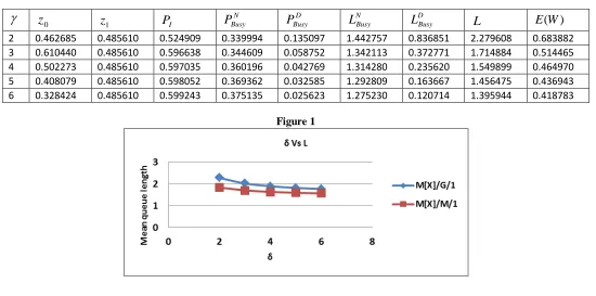
4. Numerical analysis:

In this section, numerical results related to the model of the present chapter are provided. The relation between the mean arrival

time of the disaster (δ−1), mean repair time (E(R)=

1

−

γ _{) with mean system size(L) and expected waiting time} . ) ( ) ( X E L W E λ = are examined for the model in tables 1 and 2 respectively. The graphical representations of these relations are presented in Figures 1to 4 for each model. The table values and hence the graphical representations show that the mean queue length and expected waiting time

assumed to follow Decapitated Geometric distribution of parameters (1-p). The PGF of X then, is pz

z p − −

1 ) 1 (

. It is also assumed that

normal service time S1 follows two-stage hyper exponential distribution

(

)

(

1

)

(

)

12 11

12 11

t t

e

a

e

a

µ

−µ

+

−

µ

−µ _{and slower service time S}

0

during breakdown period follows Deterministic distribution of parameter

µ

0_{. In all the tables,}

z

0_and

z

1_{respectively denote the roots}

of S g w z e z

z w g

x

x

= = − 0

) ( ( *

0( ( ( )))

µ γ

γ

where S0 is Deterministic distribution and ( ( )

) 1 ( ) ( ( )))

( ( (

12

12

11 11 *

1

z w g

a z

w g a z

w g S

x x

x

δ δ

δ _µ

µ µ

µ

+ − + +

=

where

S1 follows 2-stage hyper exponential distribution. The system size probabilities

) , ,

(P_I P_BusyN P_BusyD

, Mean queue length (L) and Expected waiting time (E(W)) are given in corresponding tables.

Table 1

(

λ

=

2

,

γ

=

2

,

p

=

0

.

4

,

a

=

0

.

32

,

E

(

S

0

)

=

1

,

E

(

S

1

)

=

0

.

441778

)

Table 2

(

δ

=

2

)

γ

z

₀

z

₁

P

_I

P

BusyN

D Busy

P

L

NBusy

D Busy

L

L

E

(

W

)

[image:8.612.33.583.349.622.2]

2 0.462685 0.485610 0.524909 0.339994 0.135097 1.442757 0.836851 2.279608 0.683882 3 0.610440 0.485610 0.596638 0.344609 0.058752 1.342113 0.372771 1.714884 0.514465 4 0.502273 0.485610 0.597035 0.360196 0.042769 1.314280 0.235620 1.549899 0.464970 5 0.408079 0.485610 0.598052 0.369362 0.032585 1.292809 0.163667 1.456475 0.436943 6 0.328424 0.485610 0.599243 0.375135 0.025623 1.275230 0.120714 1.395944 0.418783

Figure 1

δ

z

0

z

1

P

I

N Busy

P

D

Busy

P

N

Busy

L

D

Busy

L

L

E

(

W

)

Figure2

Figure3

Figure4

V. CONCLUSION

Kim and Lee (2014)[16] analysed an M/G/1 queueing system with disasters and working breakdowns. In this model it is assumed that the breakdown server is sent to repair facility and is replaced by a slow server till the server is fixed. The author analysed a batch arrival queueing system MX/G/1 with disasters and working breakdowns and derived the steady state system size distributions and some important performance measures for the model. It is verified that when the mean batch size E(X)=1, the results obtained is exactlycoincide with the results of Kim and Lee (2014).

REFERENCES

[1] Towsley, D. and Tripathi, S.K. (1991),“A single server priority queue with server failures and queue flushing”, Oper. Res. Lett., 10, 353-362. [2] Jain, G. and Sigman, K. (1996), “A Pollaczeck-Khinchine formula for M/G/1 queues with disasters”, J. Appl. Prob.33,1191-1200.

[3] Yang, W.S. and Chae, K.C. (2001), “A note on the GI/M/1 queue with Poisson negative arrivals”. J. Appl. Prob., 38, 1081-1085. [4] Chen, A. and Renshaw, E. (1997), “The M/M/1 queue with mass exodus and mass arrivals when empty”, J. Appl. Prob., 34, 192-207. [5] Chao, X. (1995), “A queueing network model with catastrophes and product form solution”, Oper. Res. Lett., 18, 75-79.

[6] Kyriakidis, E.G. and Abakuks, A. (1989), “Optimal pest control through catastrophes”, J. Appl. Prob. 27, 873-879.

[8] Yang, W.S., Kim, J.D. and Chae, K.C. (2002), “Analysis of M/G/1 stochastic clearing systems”, Stochastic. Anal. Appl. 20, 1083-1100.

[9] Atencia, I. and Moreno, P. (2004), “The discrete-time Geo/Geo/1 queue with negative customers and disasters, Com. & Oper. Res. 31,9, 1537-1548. [10] Atencia, I. and Moreno, P. (2005), “A single-server G-queue in discrete-time with geometrical arrival and service process”, Perform. Eval. 2005, 59, 85-97. [11] Yi, X.W., Kim, J.D., Choi, D.W. and Chae, K.C. (2007), “The Geo/G/1 queue with disasters and multiple working vacations”, Stochastic Models., 23, 537-549. [12] Li, Q.L. and Lin, C.(2006), “The M/G/1 processor- sharing queue with disasters”, Computers and Mathematics with Applications, 51, 987-998.

[13] Yechiali, U. (2007), “Queues with system disasters and impatient customers when system is down”, Queueing Syst., 56,195-202. [14] Sudhesh, R.(2010), “Transient analysis of a queue with system disasters and customer impatience”, Queueing Syst. 66,95-105.

[15] Chakravarthy, S.R. (2009), “A disaster queue with Markovian arrivals and impatient customers”, Applied Mathematics and Computations, 214, 48-59. [16] Kim .B.K. and Lee. D.H. (2014), “The M/G/1 queue with disasters and working breakdowns”, Applied Mathematical Modelling, 38, 1788-1798.

[17] Cox, D.R. (1955), “The analysis of non-Markovian stochastic processes by the inclusion of supplementary variables”, Proceedings of the Cambridge Philosophical Society, 51, 433-441.

AUTHORS

First Author – M.I.Afthab Begum, Professor, Department of Mathematics, Avinashilingam University, Tamil Nadu, India, [email protected]

Second Author –P.Fijy Jose, Research Scholar, Department of Mathematics, Avinashilingam University, Tamil Nadu, India, [email protected]