3018
MODEL FOR ESTIMATING BUS ARRIVAL TIMES BY
COMPARING VARIOUS CLASSIFICATIONS
1HAEKAL MOZZIA PUTRA, 2MOHAMMAD FAIDZUL NASRUDIN
1Faculty of Information Sciences and Technology, UKM, Bangi, Malaysia 2Faculty of Information Sciences and Technology, UKM, Bangi, Malaysia
E-mail: 1[email protected], 2[email protected]
ABSTRACT
The availability of reliable and precise bus information such as bus arrival times renders public transportation more attractive. It helps passengers plan by reducing their waiting times. This paper aims to develop an estimated time of arrival (ETA) model that is based on a comparison of various classifications and groupings of real-time bus tracking data. The empirical analysis results demonstrate that the prediction accuracy differs across methods, even using the same dataset. The methodology consists of three stages: literature review and identification of existing problems; development of an ETA model; and testing and comparison of models. Data are obtained from a mobile bus tracking application, namely, BasKita, in Universiti Kebangsaan Malaysia (UKM). Data such as the route ID, bus stop ID, distance, day, time interval and log time are used as features. Groupings of data are suggested, such as daily data, data by the path and the complete data set. In this paper, linear regression (LR), artificial neural network (ANN) and sequential minimum optimization regression (SMOreg) are used to develop the model. The performances of ETA models are compared via the correlation coefficient (CC) method and in terms of the root mean square error (RMSE) and the mean absolute error (MAE). This work uses moving average (MA) technical analysis on the data to reduce the estimation error. The results that are obtained using the ANN method with daily grouping and using MA as a feature are the most accurate. The results of this study contribute to the development of an ETA model that can achieve satisfactory accuracy to increase the quality of the bus service.
Keywords:Estimated Time of Arrival, Machine Learning, UKM
1. INTRODUCTION
There is no online system that provides bus information such as bus arrival times, real-time bus movements and nearby bus stations at the National University of Malaysia (UKM). Thus, passengers may wait too long at bus stations and miss buses. If the bus service can be investigated and measured, the bus service providers may further adapt more appropriate strategies to improve the quality [1], [2]. Public buses are one of the most widely used modes of transportation [3]. The accurate travel time estimated is necessary for passengers. Arrival time forecasting has attracted substantial attention and is expanding rapidly [4]. The estimated time of arrival (ETA) is used for precise planning. Therefore, in the development phase, it is necessary to consider various aspects such as the time range, structure, and features of data that have been collected [5], to increase the quality of the result.
Therefore, identifying the problems that occur in public bus transportation is one step towards improving the quality of service. This study aims to find several steps to improve the quality of bus services. Some of the steps are meant to find information related to preparing the arrival time model for bus passengers. As well as looking for various techniques to improve the development quality of the estimated arrival time model from various aspects.
The fundamental problem faced in the development phase of the model was the limited availability of bus data and was less than expected. This is due to the GPS error in sending locations, which is usually the case when there is an interruption in the internet network in an area [6]. This problem was also addressed by [7], most of the data obtained contain bus movement times that do not fit the timetable. In [6] study is required at least two prior bus journey data to generate the expected arrival time for the next bus. Lack of training data
can impact on the quality of the unsatisfactory estimated model. At the data collection stage, unscheduled bus movements have a less favourable impact on the development phase of the model.
The use of moving averages is intended to smooth the movement of data. We use the additional feature of the moving average feature to find the approximate time at a particular stop based on the record of bus travel data in the past.
Additionally, the development of estimated arrival models requires appropriate features or data. In the data collection phase, we have recorded various information such as bus information, driver information, route information, and user information. However, in the real world, many features can be acquired, but not all of these features can be used to complete data learning tasks. Only relevant features are used in the process of model development [8]. The feature selection method was used before the data learning process [9]. It reduces the time spent in the process of learning the data, improves the performance of ETA, and provides a better understanding of the data [10].
According to [5], [11] we found that in the development process, the models will show different results and compete with each other based on the size of the data, the number of data criteria and techniques used in development. Some techniques can provide a better result than other techniques, even using the same data set as conducted by [12]. Therefore, we propose and attempt to develop models based on various data groupings such as daily data, route data, and overall data. To obtain several models of ETA.
3019 lead to problems of uncertainty when using the same model on several available routes. To develop accurate and reliable ETA models, it can be built based on the similar time travel patterns that occurred in the past.
This research involves the development of models based on the historical data collected and real-time data. We use statistical methods to study travel time data and explain variations in travel time over the same period over several days. In other words, we use historical data and real-time data as input to model development. One of the methods used to study historical data methods is to use the linear regression method as developed by [3].
Other researchers have experimented with statistical methods as a way of learning between recent traffic patterns and historical traffic patterns. However, there are still errors in showing the expected results of actual arrival and departure times[15], [16]. Therefore, we try to find other methods of predicting future traffic conditions in various road segments and at each of the multiple intervals of the future as shown in the study [17]– [21]. In this study, we used machine learning methods such as artificial neural network (ANN) and Support Vector Machine (SVM) methods. The advantage of machine learning methods is its ability to study limited data and have a complex correlation between available data.
By considering the abovementioned, we propose a bus arrival time model that is based on a comparison of various classifications and groupings of data. The objective is (i) identifying the features that are suitable for the model development process; (b) Identifying the error reduction method in the model development process, and (c) comparing the results for each model that are based on multiple classifications and groupings of data.
Based on the literature review, it found that there are no studies that have been developed the estimated arrival time model with various classification method such as; Linear Regression, Artificial Neural Network, and SMOreg. Moreover, we break down the data into several segments to learn the movement of data based on daily data, route data, and overall data. As a result, we found that the study conducted could provide several model choices based on multiple perspectives.
The development process of the model will be achieved with the help of WEKA tools. It is an easy, fast tool to develop the ETA model. In some research, they do the classification method in a step to learn and group the data into similar objects [16], [22]. The dataset trained with linear regression method, artificial neural network method and sequential minimum optimization regression (SMOreg) method on a separated test. Furthermore, once WEKA does classification, then the model will evaluate with correlation coefficient (CC) method, root mean square error (RMSE) method and mean absolute error (MAE) method. In the evaluation phase, the moving average feature shows a satisfactory result. Each method has a different way of train data even when using the same amount of dataset and group of data.
2. RELATED WORK
According to [23] there are several methods and techniques used to develop the ETA model. This section describes the study on the development
process, with special reference to public bus transportation.
According to [24] features selection method playing a role in the development process of ETA. Measurement of error value is a need in solving practical problems. This paper is conducted as one of the efforts in producing reliable and precise bus arrival time estimation based on data available.
2.1 Feature Selection
The feature selection phase is aimed to improve the quality of prediction along with reducing calculation time in the model’s developing process. According to [25], some researchers have used different feature selection methods in their study to develop the ETA model. According to [10] features are part of the dataset to be studied, they are used by learning algorithms to classify the dataset. There are three main methods in the feature selection: (i) embedded method (ii) wrapping method, and (iii) filter method. Embedded method is usually found in certain methods, such as the "random forest" method where the importance of each feature is estimated as a whole process of model development. Wrapping methods combine search algorithms and learning algorithms. Hill-climbing and random optimization are some examples of this method. Wrapping method has been used by [26]– [29] in their study, the hill-climbing method is a mathematical optimization technique, the iterative algorithm starts with choosing random features, then making additional combination of features until no further improvements can be found. In this study, we used the hill-climbing method with help of WEKA tool to make some combinations of features. The filtering method is represented by a search algorithm that functions as "feature selector" before the learning algorithm. The advantage of this method is the speed of the process of modelling, which is due to the reduction of irrelevant feature by learning algorithms [30]. The CFS or Correlation-based Feature Selection is an example of this method.
2.2 Moving Average
In statistics, the moving average is used to analyzing data points by creating a series of different subsets from Whole of datasets. In this research, we use moving average as an extra feature by labelled as MA. Moving averages are typically used with time series data to smooth out the movement of volatility in the short term and generate long-term trends [31]. Moving averages is the average value of previous data. MA helps to measure the current trend of movement of data. For instance, calculating MA5
which means the average value of 5 previous data. Let say we want to predict arrival time in day 6, we can calculate it based on 5 previous days or MA5 of
data.
2.3 Estimated Time of Arrival Model
3020 between the bus stop and the time spent at the bus stop. Therefore, in our research, we group the data into several parts.
Based on our study, here we summarize the chosen model that suitable with the available data, (i) Linear regression model, (ii) Artificial neural network model, (iii) Sequential Minimum Optimization Regression (SMOreg) model:
Linear regression (LR) model
According to [33] despite that, there are many new tools and improved algorithms have been developed and use more sophisticated statistical methods, the LR method is still proven to be a powerful method to solve various types of statistical problems.
Linear Regression is a statistical model. The models predict based on interdependent data using mathematical functions formed by a set of non-dependent datasets. This model works satisfactorily even if the pattern of traffic is not similar to the data pattern [15]. LR model is used to predict the result of an unknown dependent variable, then providing the values of the independent variables as a result of the expected time.
Since we have a few features as the input, linear regression algorithms with multiple inputs are described as follows:
Y is a predictor feature or the bus arrival time feature. Y is arranged in matrix
𝑌
⎝ ⎜ ⎛
𝑌 𝑌 ⋯ ⋯ 𝑌 ⎠
⎟ ⎞
(1)
X is the input feature. Various input features have been collected, for example, route, stop distance, day. The combination of features is organized into matrices to study the data.
𝑌
⎝ ⎜ ⎛
1 𝑋 𝑋 ⋯ 𝑋
1 𝑋 𝑋 ⋯ 𝑋
⋯ ⋯ 1
⋯ ⋯ 𝑋
⋯ ⋯
𝑋 ⋯ 𝑋 ⎠
⎟ ⎞
(2)
β is the coefficient that can be arranged in the 𝛼 𝑝 1 dimension matrix.
𝛽
⎝ ⎜ ⎛
α β ⋯ ⋯ 𝛽 ⎠
⎟ ⎞
(3)
𝜖 is an error, the value of 𝜖 0. However,
it is arranged in a dimension of α n dimensions
𝜖
⎝ ⎜ ⎛ 𝜖 𝜖 ⋯ ⋯ 𝜖 ⎠
⎟ ⎞
(4)
Therefore,
𝑌 𝛼 𝛽 𝑋, ⋯ 𝛽 𝑋, 𝜖 (5)
For example, if Y is the bus arrival time, X1 is the arrival time, X2 is the stop, and X3 is the day, then the model can be written
Y 15 0.8 X1 0.5 X2 3 X
LR develops mathematical model-based learning. The LR model is one of the ways to understand how movements or changes in value are interconnected with some other value. LR works by looking for lines that minimize the data.
Artificial neural network (ANN) Model
The ANN model is a machine learning-based and becoming one of the most commonly used to develop the bus's ETA model [34]–[36]. This model is developed based on various layers of learning units called artificial neurons, this process implies the ability of human intelligence to learn new things.
According to [35] ANN method learns the sample data and captures the functional relationship between one attribute and other attributes that are unknown or difficult to explain. The public transport system is very complex and very non-linear, and the ANN model has the ability to handle complex non-linear systems, so many researchers use the ANN model to predict the arrival time of the bus [37].
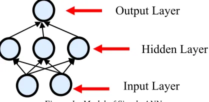
ANN or also called multi-layer perceptron (MLP) has been selected for this study as it can produce good predictions since it has enough neuron in the hidden layer as it will increase the input-output mapping capabilities. The ANN architecture typically consists of a set of nodes and connections in 3 layers as shown in Figure 1. The layers consist of an input layer, a hidden layer, and output layer. The first layer is the input layer where external information or data is received. Usually, there are one or two hidden layers are used between input-output layers to learn the data. The last layer is the output layer where problem-solving or predicted results are obtained. Actual processing in the network occurs in hidden layer nodes and output layers.
[image:3.612.315.524.562.664.2]Figure 1: Model of Simple ANN
The development of MLP consists of various artificial neurons, each neuron has a weight value which can be considered as an additional input of value. Inputs that have passed the weighting function are then entered into the activation function. The activation function performs the input ballast mapping function and transmits the input to the output neurons. It is called the activation function as it determines the strength of the relationship of each interconnected neuron.
In MLP the input data must be in a number format, for example, if you have a day feature with "Monday", "Tuesdays", "Wednesday" values. It should be changed to a number form such as "Monday = 0", "Monday = 1", "Wednesday = 2". The training algorithms for artificial neurons are called stochastic gradient descent. At this phase, a row of data is inserted in the network simultaneously as input. Furthermore, the network connecting each input neurons to produce output values. This phase is called forward pass, each row of data will be processed up to the entire data. Each output value of
Output Layer
Hidden Layer
3021 the network is compared to the other output and the value of the resulting error is also calculated. This mathematical process is called the backpropagation algorithm.
Model sequential minimum optimization regression (SMOreg)
A support vector machine (SVM) is a tool used to solve pattern matching problems and regression. It has attracted the attention of neural network researchers and mathematical programming researchers as conducted by the early developer of SMO [38]; The main reason is its ability to deliver excellent performance.
Support Vector Machine (SVM) with SMO regression algorithm (Sequential Minimum Optimization) is known as SMOreg in WEKA. SMOreg is part of a support vector machine where this nonlinear method can be used to develop an ETA model [39]. It was introduced by [40], SMOreg performs SVM regression function. Datasets can be learned using various algorithms. Learning algorithms can be selected by configuring the
RegOptimizer class in WEKA [41]. According to
[42] this method is more often used to develop time series analysis and estimated time compared with other classic statistical techniques, as this method is faster and more flexible.
In WEKA, we use SMOreg classification to study bus movement data. To train the data, the
RegSMOImproved use the pseudocode algorithms.
Pseudocode is usually used in statistics, but in SMOreg it helps this method to study and index data from multiple possible data movements. When the algorithm generates numbers at random, it is not really “random” but it is pseudocode.
2.4 Model Evaluation
According to [3] model performance evaluations is a complicated process as it involves various dimensions of aspect to be considered. Past studies suggest performance evaluations can be carried out based on statistical tests, conduct qualitative analyzes by discussing the weaknesses and advantages of the methods used, or by conducting quantitative analysis using various evaluation measures that can capture different aspects of the performance of a particular model. According to [26] different methods have different ways of evaluation depending on the error steps and the type of data. The main focus of this study is the quantitative comparison of various methods based on performance measurements, especially in terms of model accuracy. However, the identification of the appropriate method of measuring accuracy is an important issue.
The evaluation of ETA models started with data filtering, is appropriate for developing time-dependent models. It is difficult to reduce the error value from the estimated time when it is only seen from one aspect of the time-frame method. Each estimated time method has different techniques in producing ETA models. Hence, there are several methods to calculate the value of errors from each model.
2.4.1 Correlation coefficient (CC)
The use of the word correlation refers to the relationship between two or more objects. In statistics, the terminology of correlation refers to the relationship between the two variables. Correlation coefficients play an important role in statistics. With the correlation analysis, the relationship between the two variables can be examined with the help of
two-dimensional dependency measurements [41], [43]. CC usually used in calculating quantitative data as follows.
𝑟 ∑ ̅
∑ ̅ ∑ (6)
Where 𝑛 is a number of data. 𝑥 , 𝑦 are the individual sample feature indexed with t.
∑ 𝑥 ;
2.4.2 Min absolute errors (MAE)
According to [44] statistics are combinations of tools and datasets, then researchers must choose the most appropriate tool to answer the questions that they face. In this case, mean absolute error (MAE) is a method or tool that is widely used in model evaluation. MAE measures the average error value predicted and compares it with the original value, regardless of their direction [22]. It is an average of the test value of the absolute difference between predicted time and actual value in which all individual differences have the same weight [5]. The definition of MAE is as follows. To evaluate MAE, the error value should be as small as possible [22].
𝑀𝐴𝐸 ∑ 𝑌 𝑌 (7)
Where 𝑌 is a predicted time value, 𝑌 is observed value, 𝑛 is a number of data.
2.4.3 Root mean square error (RMSE)
This method is one of the most popular in the time anticipated domain [24]. RMSE is used to measure the difference between the actual value and the predicted value of the model. It is calculated as a square root value of the total difference of the original value and the estimated time of the result from the algorithm and probability vector representing the actual class of all cases [5]. RMSE is one of the most widely used error-calculation methods in environmental literature [45].
𝑅𝑀𝑆𝐸 ∑ (8)
3. METHOD
The research methodology is an action plan from several initial questions to ending with some conclusions as a result. Part of the process of research methodology is to select the appropriate method according to research questions and available data materials or possibly those that have been collected.
3022
Figure 2: Methodology of The Research
3.1 Literature Review
This study relates to provide the bus arrival time information at UKM campuses. It involves studying various literature related to the development of the ETA model. This study is focused on model development based on the comparison of various classification and group of data.
3.2 Model Development
In this phase, the study is divided into two processes: (i) Data collection: it has been done by the mobile bus tracking application – BasKita. Therefore, based on the data we do the feature selection, and (iii) Developing models based on various classification and grouping data. The model development is run using WEKA software.
3.3 Model Evaluation
In the last phase, the models evaluate multiple methods such as CC methods, MAE methods and RMSE methods with the help of WEKA software. Results are presented in the form of statistical data.
4. MODEL DEVELOPMENT
[image:5.612.338.507.516.813.2]In this part, we discuss the step of model development. The flowchart shown in Figure 3 is the overview of this study. The detail of this flowchart discussed below sub-topic.
Figure 3: Flow Chart of Model Development
Set Data
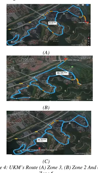
In this study, bus services at Universiti Kebangsaan Malaysia (UKM) was chosen as a place for data collection. In UKM, there are 15 buses operating and there are 3 routes to be studied covering zone 2, zone 3 and zone 6. Where zone 3 has 26 bus stops; zone 2 has 26 bus stops; zone 3 has 22 bus stops; Each route has a different pattern, as shown in Figure 4 below.
(A)
(B)
(C)
Figure 4: UKM’s Route (A) Zone 3, (B) Zone 2 And (C) Zone 6
Therefore, we develop a mobile application to collect the data. Baskita mobile application consists of three main parts that are driver’s applications, user’s applications, and web-based systems for administrators to manage bus routines. Baskita has been tested and implemented in collaboration with the UKM transport unit.
The driver's application is created specifically for the bus driver in UKM. The Driver’s
Literature Review
• Literature Review • Problem Statement • Identify Objectives • Introduction to ETA model
Model Development
• Data collection and feature selection • Development of proposed model based on
various classification and grouping of data
Model Evaluation
• Evaluation of model Based on Classifier and Data Grouping
Dataset
Pre-process
Feature Selection
Data Grouping
Daily Route Whole
Data Training and data
testing
Evaluation
Coefficient Correlation
Mean Absolute Error
Root Mean Square Error
ETA Model Classification
Linear Regression
Artificial Neural Network
[image:5.612.89.274.661.863.2]3023 application sending the latitude and longitude in real-time therefore users’ application and a web-based system able to locate the bus movement in real-time. The user's application needs to know the ETA of the chosen bus based on the user's location.
Baskita’s system is connected via API. All the buses are equipped with a mobile phone that has been installed with the driver’s application. Data such as route ID, bus stop ID, distance, day, bus time interval and bus arrival log time are used as features. The bus time interval was in 30-minutes interval (e.g., 07:00-07:30 as interval 1, 07:30-08:00 as interval 2).
4.2 Preprocess
Here is some step that we have done on the preprocessing part: (i) Data cleanup: Data cleanup starts with filter and reduce the incomplete data retrieved from the database. Incomplete bus journey such as dataset that contains a skipped list of bus stop then remove from the dataset. (ii) Data integration is the merging of some of the separated data. Data from various routes then combine into a set data of bus movement. (iii) Data transformation is to convert data from a certain format to the required format for machine learning. A set of data from the database then transforms into an ARFF file extension that suitable to WEKA. (iv) Data reduction is data analysis on large amounts of data that takes a very long time. So we use another filter method in WEKA to reduce the amount of data.
4.2.1 Feature selection
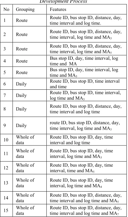
[image:6.612.90.301.534.892.2]To find the proper features we did several testing using the hill-climbing method on WEKA. This study conducted a total of 15 tests as shown in Table 1.
Table 1: Feature Selection on The ETA Model Development Process
No Grouping Features
1 Route Route ID, bus stop ID, distance, day, time interval and log time.
2 Route Route ID, bus stop ID, distance, day, time interval, log time and MA 3
3 Route Route ID, bus stop ID, distance, day, time interval, log time and MA 5
4 Route Bus stop ID, day, time interval, log time and MA
5 Route Bus stop ID, day, time interval, log time and MA 5
6 Daily Route ID, bus stop ID, time interval and time
7 Daily Route ID, bus stop ID, time interval, log time and MA 3
8 Daily Route ID, bus stop ID, distance, day, time interval and log time
9 Daily route ID, bus stop ID, distance, day, time interval, log time and MA 3
10 Whole of data Route ID, bus stop ID, day, time interval and log time
11 Whole of data Route ID, bus stop ID, day, time interval, log time and MA 3
12 Whole of data Route ID, bus stop ID, day, time interval, time and MA 5
13 Whole of data Route ID, bus stop ID, day, time interval, log time and MA 4
14 Whole of data Route ID, bus stop ID, distance, day, time interval and log time and MA 5
15 Whole of data Route ID, bus stop ID, distance, day, time interval and log time and MA 7
Based on the hill-climbing method, we have selected 5 different feature combinations route dataset, then in the daily dataset we have selected 4
feature combinations that show minimum error values, then for the whole grouping of data, we select 6 feature combinations. The reason we do several combinations is to get a different perspective of each model. Therefore we could measure the performance of each model based on multiple aspects.
After several testing that we have done, these particular 15 tests represent the lowest value of prediction error, which the feature of the model consists of route, position of current bus stop (bus stop ID), number of days (day), time log in second (log time), and moving average (MA).
4.2.2 Moving average
In the feature selection phase, we add moving average features as an extra feature. The moving average is obtained by taking the average of a subset of other data (time series) in a row. Then the subset is calculated by "moving forward"; excluding the first number of the series and including the next value in the subset. Moving average is usually used with time series data to identify long-term trends or short term trends.
The formula 𝑀 ⋯
∑ 𝑌 used to calculate the moving average
(MA).
Table 2: Moving Average Example
Bus stop ID interval Time Log time MA3
1 2 27243 0
2 2 27475 0
3 2 27671 0
4 2 27732 27463
5 2 27758 27626
6 2 27857 27720
Based on the formula, here we calculate the MA3 for bus stop number 4, 𝑀𝐴
27463. In model development, we predict the MA3 value used as a result.
4.3 Data Training and Testing
According to [46] there are two main issues related to model development. First, the dataset must be labelled correctly. Second, we need different data to determine the pattern of different traffic. Testing datasets are arranged based on training datasets.
Training data and testing data are used as the main part process of developing ETA models. Training data used for model learning the data and testing data is used to evaluate the capabilities of ETA models or to measure estimation performance. WEKA provides percentage data splitting on the test option part. It is easier for the researcher to split data using this tool.
3024
Figure 5: Data Training and Data Testing Splitting
4.4 Data Grouping
According to [12] grouping data into multiple data segments can reduce the error rate when building the model. The data are then grouped into three parts: (i) daily data set (Monday, Tuesday, Wednesday, Thursday, Friday, Saturday and Sunday); (ii) route data set (zone 2, zone 3 and zone 6); and (iii) the data set as a whole. After we do preprocessing of data, there are only 996 left. Therefore we divide the data based on the group of data.
a. The daily dataset: There were 39 data on Sunday; 193 data on Monday; 172 data on Tuesday; 189 data on Wednesday; 150 data on Thursday; 190 data on Friday; 63 data on Saturday. With a total of 996 data.
b. The route dataset: There are 35 data for zone 2, then there are 525 data for zone 3 routes; and there are 436 data on zone 6. With a total of 996 data.
c. Data grouping to the whole means that data collected as much as 996 data is examined in its entirety without any breakdown of daily data groups and routing data.
4.5 Data Classification and Model Evaluation
This part is the development process where we train all the datasets. We classify the data with three different methods which are linear regression (LR), artificial neural network (ANN) and Model Sequential Minimum Optimization Regression (SMOreg).
4.5.1 Linear regression (LR)
Linear regression is one of the most well-known and easy-to-understand algorithms in statistics. It is used as a model to understand the relationship between the input and output of the feature.
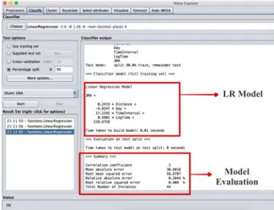
In the section below we describe the use of linear regression methods in WEKA tools as shown in Figure 6. The model uses route grouping data (Zone 3) and uses the MA3 moving average feature.
LR works by estimating the coefficients to understand the value that best suits the training data.
Linear regression modelling step:
1. Click the "Choose" button and select "Linear
Regression" under the "function" group.
2. Click on the name of the algorithm to check the configuration of the algorithm.
3. Click "OK" to close the algorithm configuration.
4. Click on "Percentage Split" then enter the value "70%".
5. Click the "Start" button to run the linear regression model development.
The performance of the linear regression model can be reduced if the training data consist of input features that are closely related or overfitting. WEKA can detect and remove overfitting inputs automatically by setting
eliminateColinear-Attributes to True.
In addition, attributes that are not related to output variables can also negatively affect model performance. WEKA can automatically run the feature selection method, which is by setting
attributeSelectionMethod to the feature selection
[image:7.612.313.509.338.449.2]method. However, in this study, we have disabled this method because it has been done manually in feature selection through the hill-climbing method, so there is no need for feature selection in this development process.
Figure 6: Linear Regression Model Development
The model development processes and model evaluation are shown in Figure 7. Furthermore, the value of the CC, MAE and RMSE errors of the model is also shown in Figure 7. The example of the linear regression modelling process, we use 7 features based on the hill-climbing method previously implemented. The features used to build the model are "routeID" "BusStopID", "Distance", "Day", "TimeInterval" , "LogTime", and "MA3".
[image:7.612.312.510.700.852.2]There are 436 sets of data to be analyzed. The data set is divided into 90% or 392 data as training data and 10% or as much as 44 data as test data. The model development process takes 0.01 seconds. The average error or MAE from the development of this model is 30.8, with a correlation of 1 coefficient that means a strong correlation of each feature in the training data set.
Figure 7: Linear Regression Model Evaluation
4.5.2 Artificial neural network
3025 data (Zone 3) and uses the MA3 moving average
feature.
The ANN is a complex set of algorithms that are widely used in forecasting because many parameter configurations can be used. The development of ANN or Multi-Layer Perceptron (MLP) is explained in Figure 8:
1. Click the "Choose" button and select "MultilayerPerceptron" under the "function"
group.
[image:8.612.322.513.107.258.2]2. Click on the algorithm name to check the algorithm configuration.
Figure 8: ANN Model Configuration
WEKA allows users to determine the nerve network structure used by the model. However, WEKA can automatically design the network and train it on the dataset. The number of hidden layers in the hiddenLayers parameter, set with the value "a"
which means 'a' = (feature + class) / 2. The number of hidden layers is shown in Figure 9 below.
Figure 9: ANN Learning Layer
As shown in Figure 9, it can configure the learning process by specifying how much learning rate is, by setting the value of epoch, the value between 0.3 (default) and 0.1. The learning process can be adjusted with momentum (set to 0.2 by default). The following step is described below: 3. Click "OK" to close the algorithm configuration. 4. Click the "Start" button to run the algorithm in
the dataset.
The details of the development of the model are described below. The example of the ANN modeling process, we use 7 features based on the hill-climbing method previously implemented. The features used to build the model are "routeID" "BusStopID", "Distance", "Day", "TimeInterval" , "LogTime", "MA3". There are 436 sets of data to be
[image:8.612.92.294.248.373.2]learned. The data set is divided into 70% or as much as 305 data as training data and 10% or as much as 131 data as test data. The model development process takes 0.19 seconds. The average error or MAE from the development of this model is 185.9. The correlation coefficient of 0.999 means a strong correlation of each feature in the training data set or approaching value 1.
Figure 10: ANN Model Evaluation
If we compare to the previous test which is the LR model, this model shows unsatisfied results since it shows higher error value. Even with a similar dataset. If we try 90% of splitting data training it shows MAE value = 259.7 and RMSE value = 282.6.
4.5.3 Sequential minimum optimization regression (SMOreg)
The following section is an example of an ETA model development in WEKA software. The development of this SMOreg model uses route grouping data (Zone 3).
Support Vector Machines have been developed to solve binary classification problems, even there are many more methods to use but SVM shows its ability to develop an ETA model.
SVM is developed for numerical input variables, although it automatically changes the nominal value to numerical values. Input data is also normalized before use.
The SMOreg model development stage is described as follows:
1. Click the "Choose" button and select "SMOreg" under the "function" group.
2. Click on the name of the algorithm to check the configuration of the algorithm.
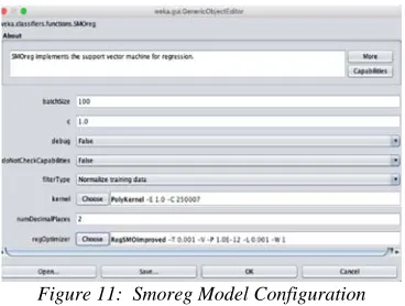
The detail of Figure 11 is described below. The parameter C, called the complexity parameter in WEKA, aims to control the flexibility in drawing the line to match the data being studied. Value 0 does not allow to cross the margin line, while the default used is 1.
The main kernel parameters in SMOreg are
Poly Kernel, which corresponds to the data using
curved or wiggly lines. Higher polynomial means higher exponential value. Polynomial kernel has a default exponent value = 1, which makes it equal to the linear kernel.
Figure 11: Smoreg Model Configuration
[image:8.612.90.290.484.620.2] [image:8.612.326.510.768.907.2]3026 1. Click "OK" to close the algorithm configuration. 2. Click the "Start" button to run the algorithm on
the dataset.
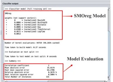
Figure 12 shows the development steps and model evaluation of the SMOreg model. The example of the ANN modelling process, we use 7 features based on the hill-climbing method previously implemented. The features used to build the model are "routeID" "BusStopID", "Distance", "Day", "TimeInterval", "LogTime", "MA3". There
[image:9.612.99.293.319.460.2]are 436 sets of data to be learned. Data sets are divided into 70% or 305 data as training data and 30% or as many as 131 data as test data. The model development process takes 0.37 seconds. The average error or MAE from the development of this model is 35.9. A correlation coefficient of 1 means a strong correlation of each feature in the training dataset.
Figure 12: Smoreg Model and Evaluation
5. RESULTS AND DISCUSSION
According to [5] model comparison analysis is a complicated process as it involves various dimensions of assessment that need to be considered. Previous studies have suggested that performance appraisals may be based on statistical tests, conducting qualitative analysis by discussing the weaknesses and advantages of the methods used, or by performing quantitative analysis using various assessment measures that capture different aspects of the performance of particular models. Different
methods have different assessment methods depending on error steps and data types. The main focus of this study is the quantitative comparison of various methods based on performance measures, especially in terms of model accuracy. However, the identification of appropriate measures in measuring accuracy is an important issue.
As discussed in the previous section, the performance of the three models was compared to select the most suitable model for predicting real-time bus arrival. In this section, we compare the model that has been developed based on classification and groping of data with several combinations of features selection and splitting test data.
Table 3, is a comparison of the test sets that have been run. Based on the "test" sub-chapter, only the method that shows the lowest error value will be selected and described in the section below. For example in "test 1", the test run is on grouping path data. The grouping of the data was tested using various methods and breakdown of the test data, and then the tests were summed and averaged. Based on these averages we select test methods and breakdowns, the rows with the lowest error values that we consider to be the preferred method and described in the "test" sub-chapter.
Based on “feature selection” in Table 1, some of the tests we add MA. We want to try how much this feature improvement the model performance. All of the features that we test based on the hill-climbing method. Furthermore, in Table 5 we conclude the MA feature, compare to testing without adding MA feature.
The step that we do on this testing is: 1. Chose the feature that available from Table 1 2. Chose the classification (LR, MLP, SMOreg) 3. Chose the data training percentage splitting
(70%, 80%, 90%)
[image:9.612.93.558.630.957.2]4. Documented each the result into one set testing
Table 3: Model Comparison
No of
train Group Method
Data percent
age CC MAE RMSE Feature
1 Route SMOReg 90% 0.9989 222.390 482.452 Route ID, bus stop ID, distance, day, time interval and log time.
2 Route LR 70% 0.9999 43.028 149.854 Route ID, bus stop ID, distance, day, time interval, log time and MA
3
3 Route LR 70% 0.9999 42.489 117.816 Route ID, bus stop ID, distance, day, time interval, log time and MA
5
4 Route LR 70% 0.9999 47.966 154.607 Bus stop ID, day, time interval, log time and MA
5 Route LR 70% 0.9999 48.224 121.758 Bus stop ID, day, time interval, log time and MA5
6 Daily NN 80% 0.9993 344.697 466.193 Route ID, bus stop ID, time interval and time
7 Daily LR 90% 0.9978 21.340 28.417 Route ID, bus stop ID, time interval, log time and MA3
8 Daily NN 90% 0.9999 250.395 295.458 Route ID, bus stop ID, distance, day, time interval and log time
9 Daily NN 90% 1 20.476 27.627 route ID, bus stop ID, distance, day, time interval, log time and MA
3
10 of data Whole SMOReg 80% 0.9976 361.666 932.894 Route ID, bus stop ID, day, time interval and log time
11 of data Whole LR 70% 0.9999 62.597 196.600 Route ID, bus stop ID, day, time interval, log time and MA
3
12 of data Whole LR 70% 0.9999 59.036 132.753 Route ID, bus stop ID, day, time interval, time and MA5
13 of data Whole SMOReg 70% 0.9999 48.397 158.122 Route ID, bus stop ID, day, time interval, log time and MA
4
14 of data Whole SMOReg 70% 1 48.852 129.465 Route ID, bus stop ID, distance, day, time interval and log time and MA 5
3027 In this section, we describe the comparison of each testing model. The following table contains the values of the 15 tests that have been done. In a test, there are several models built based on classification and grouping of the dataset. In Table 3, only the lowest error value of each testing set that we've inserted. Thus, if in one test we try with several classification methods and several data splitting with a similar feature, we only insert the lowest error value of that test into this table.
The comparable segment is the error value of CC, MAE, and RMSE. In Table 3, there are 7 main columns: " No of testing", "Group", "Method", " Data percentage", “CC”, "MAE", "RMSE" and "Features". The “No of testing” column shows the sequence of tests that have been run. The “group” column is the grouping of the data selected on the test. The “Method” column is a method used to develop the model. The “Data percentage” column is a split of training data in percent. The “CC” column is the correlation value of the dataset. The “MAE” column is the error value. The “RMSE” column is the error value. The “Feature” column is a combination of features that have been previously selected based on hill-climbing method, and run on the test.
Referring to Table 3, here we discuss the comparison of models that have been developed based on the data grouping:
a. Route dataset grouping: at test 1 we use the SMOReg method and data training splitting to 90% as well as the use of routeID, bus stop ID, distance, days, time intervals and log time feature giving unsatisfactory results. Test 1 shows the error value of MAE = 222.389 and error value of RMSE = 482,452, error value in this test is the highest error value on route data grouping. Next, we compared with test 3, the use of the LR method with data distribution to 70% and using routeID, bus stop ID, distance, day, time interval, and MA5 features showed a more
satisfying result. This is indicated by the error value of MAE = 42.489 and error value of RMSE = 117.816, the error value in this test is the lowest error value in the grouping of route
dataset. By using a moving average feature in test 3 compare to without using the moving average feature in test 1 shows lower MAE and RMSE error value.
b. Daily dataset grouping: in test 6 we use routeID, bus stop ID, time interval and log time feature and using the NN method and splitting training data to 80% shows a less satisfactory result. This is indicated by the error value of MAE = 344,697 and the error value of RMSE = 466,193, the error value in this test is the highest error value in the daily data grouping. We then compared to test 9 using the NN method and splitting training data to 90% using the routeID, bus stop ID, distance, day, time interval, and MA3 features which showed a more satisfying
result. This is indicated by the error value of MAE = 20.476 and error value of RMSE = 27.627, the error value in this test is the lowest error value in the daily data grouping. Comparison of using moving average feature on tests 9 and 7 as well as the test without moving average feature in tests 6 and 8 show less MAE and RMSE error value.
c. The grouping of Whole of data: in test 10 using route ID, bus stop ID, day, time interval and log time features the SMOReg method and splitting training data to 80% shows less satisfactory results. This is indicated by the error value of MAE = 361,666 and the error value of RMSE = 932.894, the error value in this test is the highest error value in the Whole of data grouping. On test 14 we use the SMOReg method and splitting training data to 70% by using route ID, bus stop ID, distance, day, time interval and log time and MA5 features show more satisfactory results.
This is indicated by the error value of MAE = 48,852 and error value of RMSE = 129,465, the error value in this test is the lowest error value in the Whole of data grouping. Comparison of using moving average feature on tests 11, 12, 13, 14 and 15 and test without moving average feature in test 10 showed less MAE and RMSE error value.
Table 4: Model Comparison Based On Grouping of Dataset
No testing No of Group Method
Data percen
tage CC MAE RMSE Feature
1 3 Route LR 70% 0.999 42.489 117.816 Route ID, bus stop ID, distance, day, time interval, log time and MA5
2 9 Daily NN 90% 1 20.476 27.627 Route ID, bus stop ID, distance, day, time interval, log time and MA3
3 14 of data Whole SMOReg 70% 1 48.852 129.465
Route ID, bus stop ID, distance, day, time interval and log time and MA5
In summary, we have selected three tests that show the lowest MAE and RMSE values for each data grouping as shown in Table 4. All the tests use the average moving feature in the development process.
Based on Table 4, we can conclude that test 9 shows a satisfactory model. It shows the lowest error value of MAE and RMSE from the whole of the test set. This test uses artificial neural network methods or in WEKA called multilayer perceptron (MLP). Features used based on hill-climbing feature selection are route ID, bus stop ID, distance, day, time interval, log time and MA3. Error value MAE =
20.4762 and error value RMSE = 27.6267. The test
uses the moving average feature as an additional feature in model development.
3028
Table 5: Average Result Using MA
No Grouping
Average result without MA Average result using MA
MAE RMSE MAE RMSE
1 Route 222.39 482.45 45.43 136.01
2 Daily 297.55 380.83 20.91 28.02
3 Whole of data 361.67 932.89 54.15 154.88
Based on the study that we have done, we conclude that Linear regression models have been used in regions with minimum congestion numbers. The model uses a traffic pattern that is very similar to the previous traffic pattern. This model can be used when there is extensive historical data by looking at comparisons of travel time throughout the day. Many researchers evaluate the performance of their models in terms of accuracy. Researchers typically use data that has been collected for days, weeks, and even months, taking into account the current traffic features. We have chosen this model because of its ease and speed in studying historical data. It has been proven to produce a model of expected arrival times in a tight traffic pattern, which is consistent with the situation in the data we collect. The Artificial Neural Network (ANN) model in its application is widely used in urban areas. The ability of the ANN method in studying nonlinear data shows effective results in solving optimization problems. We have chosen this model because of its advantages in studying complex data. The problem we face is the limited amount of data. So with all the advantages inherent in studying the data, it is hoped to produce the estimated arrival time with a satisfactory level of accuracy.
In summary, linear regression models are judged to be able to compete when using the appropriate features and to obtain data in areas with traffic patterns that tend to be static. Linear regression models can determine satisfactory bus arrival times, so there is no need for complex time expectancy models. However, it can be said that the ANN models, linear regression and SMOreg are used to provide better real-time travel information as they are more effective in dealing with non-linear relationships between factors that influence travel time expectancy.
Additionally, to improve the expected model of arrival time, researchers can group the data into several segments so that they can study the data from a variety of different perspectives. We have found that each model with different grouping and the use of different features shows very competing results. Further, we use the moving average feature in conjunction with the existing features “Route ID”, “bus stop ID”, “distance”, “day”, “time interval”, “log time” and “Moving Average”. The moving average feature works to fine-tune the movement of data based on the data available in the past.
On the other hand, it can be concluded that each classification method has a different way to learn the data. By following the research of [12] and [47], we can improve much more bus arrival time model by adding more multiple groups of data and adding a moving average feature. the data learn with more classification methods such as statistical method (linear regression) and machine learning method (artificial neural network and SMOReg). It ends up with a satisfactory model, and prove that ANN is still one of the best methods in developing estimated time of arrival model.
6. CONCLUSIONS
Providing reliable and accurate arrival time information is a necessity for both service providers and passengers. An accurate ETA information is considered as an important step in improving the quality of bus services, especially in the UKM campus area. Various methods and data grouping have been proposed to develop the ETA.
The objective of the study is to identifying the features that are suitable for the model development process, Identifying the error reduction method for the ETA method and comparing the results for each model that are based on multiple classifications and groupings of data. The methodology of the study was conducted based on three stages: literature review and identify existing problems; development of the ETA model; and Testing the models.
The problem that we encountered during the model development is the limitation of data collection due to human error and system error. Thus, the data that has been collected for 3 months cannot be fully utilized. There is a lot of uncomplete bus journey data record that should be removed. In this study only 996 data are eligible. The complete data means the system record the bus journey data from the first stop and pass each stop according to the set schedule until the last stop.
Therefore we overcome it in several ways. The purpose of grouping data into multiple data segments is to understand the pattern of data movement, it can also reduce the error value of the model in the development process. This is proven by tests that have been done during model evaluation.
In this study, we use the mobile bus tracking app - BasKita to collect the data such as route, bus stop, distance, day, time interval, and bus arrival time. ETA is used by passengers when they travel to another bus stop. The data that we collected then used as input in building the ETA model.
The hill-climbing method is used as a method of feature selection in the development process. The development process of the ETA model is proposed by a group the data into multiple data segments: daily data, route data, and Whole of dataset.
Based on the grouping of the dataset, it provides several model options to the researcher. In addition, the ability of each classification method also provides different results based on data grouping.
This study has been using WEKA's existing software in the development and testing process of the model. Feature selection, data cleaning, data training, and testing are all using WEKA software as it is fast and easy to use.
3029 mean absolute error (MAE) method. The model development and evaluation process in this study uses a combination of training and testing data splitting into 70%, 80%, 90% with the purpose of obtaining several evaluation options based on a dataset that we collected.
Based on the testing that we conducted on 15 sets of test found that; the Linear Regression method has shown its dominance in developing an ETA model, which there are 7 tests showing low error values; Furthermore, the SMOReg method using Vector Supporting Machine (SVM) with the SMO (Sequential Minimum Optimization) algorithm shows satisfactory results, which there are 5 tests showing low error values; at the end of the ANN method shows the number of unsatisfactory tests which there were only 2 tests which showed a low error value. However, the ANN method has its advantages in studying difficult data and is capable of providing the lowest error value compared to others.
Based on Table 3, we can conclude that test number 9 shows the most satisfactory model. It shows the lowest MAE and RMSE error value from the rest of the test. This test uses artificial neural network methods or in WEKA called multilayer perceptron (MLP). Features used based on hill-climbing feature selection are routeID, stop, distance, day, time interval, time and MA3. Error
value MAE = 20.4762 and error value RMSE = 27.6267.
Based on Table 5, the use of the moving average feature shows a more satisfactory result compared to the non-moving average. The moving average feature function to reduce the error value of the model even with a small amount of data training set.
Based on the study that has been done in the section above it can be concluded that the study has successfully conducted research on the development of the estimated arrival time model based on various classifications and groupings of data. The results of this study can be summarized as follows: Successfully studied several reliable models of estimated arrival time by incorporating several appropriate classification models; Shows detailed results of different sets of groupings; Can show results using multiple sets of sizes according to each set of groups studied; Can show better expected results by using moving averages in a set of study attributes.
In the future, in order to improve the quality of the estimated time of arrival model, it is necessary to conduct study using more data and features, such as traffic conditions, traffic lights, route conditions, number of vehicles on the road, travel time, weather conditions, vehicle driving style, stop time at each stop, number of passengers and others.
There are many other methods that can be used to develop the ETA model such as the Kalman filtering model, hybrid model, naive bayes, autoregressive integrated moving average (ARIMA) and others. Therefore, based on this study, researchers are expected to develop models for other types of vehicles in other areas with suggested to train the data with multiple grouping of data and use of moving average.
ACKNOWLEDGMENT
This work was supported by UKM under grant no. FRGS/1/2016/ICT02/UKM/02/1.
REFERENCES
[1] D. Crout, “Accuracy and Precision of the Transit Tracker System,” Transp. Res. Rec. J.
Transp. Res. Board, vol. 1992, pp. 93–100,
2007.
[2] L. Shi, “Bus Arrival Time Reliability Analyses and Dynamic Prediction Model Based on Multi-source Data,” 2016.
[3] D. Nissimoff, “Real-time learning and prediction of public transit bus arrival times,” 2016.
[4] Y. Lv, Y. Duan, W. Kang, Z. Li, and F. Y. Wang, “Traffic Flow Prediction with Big Data: A Deep Learning Approach,” IEEE Trans.
Intell. Transp. Syst., vol. 16, no. 2, pp. 865–
873, 2015.
[5] N. Mehdiyev, D. Enke, P. Fettke, and P. Loos, “Evaluating Forecasting Methods by Considering Different Accuracy Measures,”
Procedia Comput. Sci., vol. 95, pp. 264–271,
2016.
[6] I. Madras, "Development of a Real-Time Bus Arrival Time Prediction System under Indian Traffic Conditions," Cent. Excell. Urban
Transp., no. June, 2016.
[7] M. Kormaksson, L. Barbosa, M. R. Vieira, and B. Zadrozny, “Bus Travel Time Predictions Using Additive Models,” 2014 IEEE Int. Conf.
Data Min., pp. 875–880, 2014.
[8] S. Gnanambal, “Classification Algorithms with Attribute Selection : an evaluation study using WEKA,” vol. 3644, pp. 3640–3644, 2018. [9] L. Koc, T. A. Mazzuchi, and S. Sarkani, “A
network intrusion detection system based on a Hidden Naïve Bayes multiclass classifier,”
Expert Syst. Appl., vol. 39, no. 18, pp. 13492–
13500, 2012.
[10] G. Chandrashekar and F. Sahin, “A survey on feature selection methods,” Comput. Electr. Eng., vol. 40, no. 1, pp. 16–28, 2014.
[11] B. Xu and J. Ouenniche, “Performance evaluation of competing forecasting models: A multidimensional framework based on MCDA,” Expert Syst. Appl., vol. 39, no. 9, pp.
8312–8324, 2012.
[12] P. Balasubramanian and K. R. Rao, “An Adaptive Long-Term Bus Arrival Time Prediction Model with Cyclic Variations,” J.
Public Transp., vol. 18, no. 1, pp. 1–18, 2015.
[13] O. B. Downs, C. H. Chapman, and A. Barker, “Dynamic time series prediction of future traffic conditions,” Google Patents, 2011.
[14] H. Chang, D. Park, S. Lee, H. Lee, and S. Baek, “Dynamic multi-interval bus travel time prediction using bus transit data,”
Transportmetrica, vol. 6, no. 1, pp. 19–38,
2010.
[15] M. Altinkaya and M. Zontul, “Urban Bus Arrival Time Prediction: A Review of Computational Models,” Int. J. Recent
Technol. Eng., vol. 2, no. 4, pp. 2277–3878,
2013.
[16] M. Čelan and M. Lep, “Bus arrival time prediction based on network model,” Procedia
Comput. Sci., vol. 113, pp. 138–145, 2017.
[17] S. Eken and A. Sayar, “A Smart Bus Tracking System Based on Location- Aware Services and QR Codes,” pp. 1–5, 2014.
[18] R. A. Kadir, Y. Shima, R. Sulaiman, and F. Ali, “Clustering of public transport operation using K-means,” 2018 IEEE 3rd Int. Conf. Big Data
Anal., no. Ivi, pp. 427–432, 2018.
3030 using Android Application,” vol. 3, no. 4, pp. 414–418, 2018.
[20] S. Maiti, A. A. Pal, A. A. Pal, T. Chattopadhyay, and A. Mukherjee, “Historical Data based Real Time Prediction of Vehicle Arrival Time,” 17th Int. IEEE Conf. Intell.
Transp. Syst., pp. 1837–1842, 2014.
[21] M. Zaki, I. Ashour, M. Zorkany, and B. Hesham, “Online Bus Arrival Time Prediction Using Hybrid Neural Network and Kalman filter Techniques,” Int. J. Mod. Eng. Res., vol.
3, pp. 2035–2041, 2013.
[22] R. K. R. A. Agrawal, “An Introductory Study on Time Series Modeling and Forecasting,”
arXiv Prepr. arXiv1302.6613, vol. 1302.6613,
pp. 1–68, 2013.
[23] R. Choudhary, A. Khamparia, and A. K. Gahier, “Real time prediction of bus arrival time: A review,” 2016 2nd Int. Conf. Next
Gener. Comput. Technol., no. October, pp. 25–
29, 2016.
[24] M. V. Shcherbakov, A. Brebels, N. L. Shcherbakova, A. P. Tyukov, T. A. Janovsky, and V. A. evich Kamaev, “A survey of forecast error measures,” World Appl. Sci. J., vol. 24,
no. 24, pp. 171–176, 2013.
[25] A. R. Onik, N. F. Haq, and L. Alam, “An Analytical Comparison on Filter Feature Extraction Method in Data Mining using J48 Classifier,” Int. J. Comput. Appl., vol. 124, no.
13, pp. 2–8, 2015.
[26] B. N. Alajmi, K. H. Ahmed, S. J. Finney, and B. W. Williams, “Fuzzy-logic-control approach of a modified hill-climbing method for maximum power point in microgrid standalone photovoltaic system,” IEEE Trans.
Power Electron., vol. 26, no. 4, pp. 1022–1030,
2011.
[27] R. Caruana, A. Munson, and A. Niculescu-Mizil, “Getting the most out of ensemble selection,” Proc. - IEEE Int. Conf. Data
Mining, ICDM, pp. 828–833, 2006.
[28] N. Mutoh, M. Ohno, and T. Inoue, “A method for MPPT control while searching for parameters corresponding to weather conditions for PV generation systems,” IEEE
Trans. Ind. Electron., vol. 53, no. 4, pp. 1055–
1065, 2006.
[29] M. F. Nasrudin, K. Omar, C. Y. Liong, and M. S. Zakaria, “Object signature features selection for handwritten jawi recognition,” Adv. Intell.
Soft Comput., vol. 79, no. January, pp. 689–
698, 2010.
[30] V. Kumar, “Feature Selection: A literature Review,” Smart Comput. Rev., vol. 4, no. 3,
2014.
[31] D. C. Montgomery, C. L. Jennings, and M. Kulahci, INTRODUCTION TO TIME SERIES
ANALYSIS AND FORECASTING. John Wiley
& Sons, 2015.
[32] O. Cats and G. Loutos, “Evaluating the added-value of online bus arrival prediction schemes,” Transp. Res. Part A Policy Pract.,
vol. 86, pp. 35–55, 2016.
[33] P. Wallström, “Evaluation of Forecasting Techniques and Forecast Errors With Focus on Intermittent Demand,” 2009.
[34] J. Amita, S. S. Jain, and P. K. Garg, “Prediction of Bus Travel Time Using ANN: A Case Study in Delhi,” Transp. Res. Procedia, vol. 17, no.
December 2014, pp. 263–272, 2016.
[35] Z. K. Gurmu, “A Dynamic Prediction of Travel Time for Transit Vehicles in Brazil Using GPS Data,” Transit, p. 150, 2010.
[36] T. Yin, G. Zhong, J. Zhang, S. He, and B. Ran, “A prediction model of bus arrival time at stops with multi-routes,” Transp. Res. Procedia, vol.
25, pp. 4627–4640, 2017.
[37] H. Xu and J. Ying, “Bus arrival time prediction with real-time and historic data,” Cluster
Comput., vol. 20, no. 4, pp. 3099–3106, 2017.
[38] J. C. Platt, “Sequential Minimal Optimization : A Fast Algorithm for Training Support Vector Machines,” pp. 1–21, 1998.
[39] Kavitha, Varuna, and Ramya, “A Comparative Analysis on Linear Regression and Support Vector Regression,” Ieee, 2016.
[40] S. K. Shevade, S. S. Keerthi, C. Bhattacharyya, and K. R. K. Murthy, “Improvements to the SMO Algorithm for SVM Regression,” IEEE
Trans. neural networks, vol. 11, no. 5, pp.
1188–1193, 2000.
[41] V. Choubey, “Time Series Data Mining in Real Time Surface Runoff Forecasting through Support Vector Machine,” Int. J. Comput.
Appl., vol. 98, no. 3, pp. 23–28, 2014.
[42] E. Be, P. U. Elektroprivreda, and H. Sarajevo, “Machine learning techniques for short-term load forecasting,” no. September, pp. 1–73, 2015.
[43] R. M. Rodríguez, L. Martínez, V. Torra, Z. S. Xu, and F. Herrera, “Hesitant Fuzzy Sets: State of the Art and Future Directions,” Int. J. Intell.
Syst., vol. 29, no. 2, pp. 495–524, 2014.
[44] T. Chai and R. R. Draxler, “Root mean square error (RMSE) or mean absolute error (MAE)? -Arguments against avoiding RMSE in the literature,” Geosci. Model Dev., vol. 7, no. 3,
pp. 1247–1250, 2014.
[45] C. J. Willmott and K. Matsuura, “Advantages of the mean absolute error (MAE) over the root mean square error (RMSE) in assessing average model performance,” Clim. Res., vol.
30, no. 1, pp. 79–82, 2005.
[46] M. Soysal and E. Guran, “Machine learning algorithms for accurate flow-based network traffic classification : Evaluation and comparison,” Perform. Eval., vol. 67, no. 6, pp.
451–467, 2010.
[47] M. As and T. Mine, “Dynamic Bus Travel Time Prediction Using an ANN-based Model,”
Proc. 12th Int. Conf. Ubiquitous Inf. Manag.