The kinematics and morphology of solar coronal mass ejections

(1)

Jason P. Byrne, B.A.(Mod.)

School of Physics

University of Dublin, Trinity College

A thesis submitted for the degree of

PhilosophiæDoctor (PhD)

September 2010

(2)

(3)

at Earth and other locations in the heliosphere, so it is important

to understand the physics governing their eruption and propagation.

However the diffuse morphology and transient nature of CMEs makes

them difficult to identify and track using traditional image

process-ing techniques. Furthermore, the true three-dimensional geometry

of CMEs has remained elusive due to the limitations of coronagraph

plane-of-sky images with restricted fields-of-view. For these reasons

the Solar Terrestrial Relations Observatory (STEREO) was launched

as a twin-spacecraft mission to fly in orbits ahead and behind the

Earth in order to triangulate independent observations of CME

struc-ture. It is the first time CMEs have been observed from vantage points

off the Sun-Earth line and each spacecraft carries an instrument suite

designed to image from the low solar corona out to the orbit of Earth

in order to observe and study CME propagation towards Earth.

In this thesis the implementation of multiscale image processing

tech-niques to identify and track the CME front through coronagraph

im-ages is detailed. An ellipse characterisation of the CME front is used

to determine the CME kinematics and morphology with increased

precision as compared to techniques used in current CME catalogues,

and efforts are underway to automate this procedure for applying to

a large number of CME observations for future analysis. It was found

that CMEs do not simply undergo constant acceleration, but rather

(4)

were derived from plane-of-sky measurements with no correction for

how the true CME geometry and direction affect the kinematics and morphology observed.

With the advent of the unique dual perspectives of the STEREO

spacecraft, the multiscale methods were extended to an elliptical

tie-pointing technique in order reconstruct the front of a CME in three-dimensions. Applying this technique to the Earth-directed CME of

12 December 2008 allowed an accurate determination of its true

kine-matics and morphology, and the CME was found to undergo early

acceleration, non-radial motion, angular width expansion, and

aero-dynamic drag in the solar wind as it propagated towards Earth. This

study and its conclusions are of vital importance to the fields of space

weather monitoring and forecasting.

*This is the online version of this thesis which has reduced quality

(5)

(6)

I am hugely grateful to my supervisor Peter Gallagher. You have been a constant source of inspiration, and it has been an absolute pleasure

to work with you.

A big thank you goes to Alex Young for your guidance and support

during my time at Goddard. Working in NASA was everything I could have hoped it would be. Thank you also to James McAteer,

Jack Ireland, Angelos Vourlidas, everyone in the SOHO and STEREO

teams and extended Goddard network. Your guidance and helpful

discussion have been invaluable.

A collective thank you goes to Shane Maloney, James McAteer, Jose Refojo and Peter Gallagher for the huge amount of time and effort

you contributed to achieving the final stages of work in this thesis.

A massive thank you goes to all the staff and students in the

Astro-physics Research Group in Trinity College, including those who have

since left. You made my time here as enjoyable as possible, and I’m sorry it has to come to an end.

And finally, a heartfelt thank you to my friends and family. You mean

(7)

List of Figures xi

List of Tables xxxi

1 Introduction 1

1.1 The Solar Interior . . . 2

1.2 The Solar Atmosphere . . . 7

1.2.1 Photosphere . . . 8

1.2.2 Chromosphere . . . 9

1.2.3 Corona . . . 12

1.2.4 Solar Wind . . . 16

1.2.5 Space Weather . . . 20

1.3 Coronal Mass Ejections . . . 23

1.3.1 Magnetohydrodynamic Theory . . . 26

1.3.1.1 Maxwell’s Equations . . . 26

1.3.1.2 Fluid Equations . . . 27

1.3.1.3 The Induction Equation . . . 28

1.3.1.4 The Magnetic Reynolds Number . . . 29

1.3.1.5 Magnetic Reconnection . . . 30

1.3.2 Theoretical CME Models . . . 33

1.3.2.1 Catastrophe Model . . . 36

1.3.2.2 Toroidal Instability . . . 38

(8)

1.3.3 CME Observations . . . 44

1.3.3.1 Thomson Scattering . . . 44

1.3.3.2 CME Kinematics & Morphology . . . 50

1.4 Outline of Thesis . . . 59

2 Instrumentation 61 2.1 SOHO/LASCO . . . 62

2.2 STEREO/SECCHI . . . 66

2.2.1 EUVI . . . 68

2.2.2 COR1 . . . 69

2.2.3 COR2 . . . 71

2.2.4 Heliospheric Imagers . . . 71

2.3 CCD Detectors . . . 74

2.4 Coordinate Systems . . . 78

2.4.1 Heliographic Coordinates . . . 78

2.4.2 Heliocentric Coordinates . . . 79

2.4.2.1 Heliocentric Earth Equatorial (HEEQ) . . . 80

2.4.2.2 Heliocentric Earth Ecliptic (HEE) . . . 80

2.4.2.3 Heliocentric Aries Ecliptic (HAE) . . . 80

2.4.3 Helioprojective Coordinates . . . 81

3 Detecting and Tracking CMEs 83 3.1 CME Detection Catalogues . . . 84

3.1.1 CDAW . . . 85

3.1.2 CACTus . . . 86

3.1.3 SEEDS . . . 89

3.1.4 ARTEMIS . . . 91

3.2 Multiscale Filtering . . . 94

3.3 Automated Multiscale CME Detection . . . 99

3.3.1 Normalising Radial Graded Filter (NRGF) . . . 100

3.3.2 Thresholding . . . 102

3.3.3 Faint CMEs and Streamer Interactions/Deflections . . . . 107

(9)

4.2.1 3-Point Lagrangian Interpolation . . . 118

4.3 Results . . . 121

4.3.1 Arcade Eruption: 2 January 2000 . . . 122

4.3.2 Gradual/Expanding CME: 18 April 2000 . . . 124

4.3.3 Impulsive CME: 23 April 2000 . . . 127

4.3.4 Faint CME: 23 April 2001 . . . 127

4.3.5 Fast CME: 21 April 2002 . . . 130

4.3.6 Flux-Rope/Slow CME: 1 April 2004 . . . 130

4.3.7 STEREO-B Event: 8 October 2007 . . . 132

4.3.8 STEREO-A Event: 16 November 2007 . . . 135

4.4 Discussion & Conclusions . . . 135

5 Propagation of an Earth-Directed CME in Three-Dimensions 139 5.1 Introduction . . . 140

5.2 The STEREO Era . . . 142

5.3 Elliptical Tie-Pointing . . . 147

5.3.1 SOHO as a Third Perspective . . . 151

5.4 Earth-Directed CME . . . 153

5.5 Results . . . 163

5.5.1 3D Error Propagation . . . 165

5.5.2 Prominence & CME Acceleration . . . 167

5.5.3 Non-radial Prominence & CME Motion. . . 167

5.5.4 CME Angular Width Expansion . . . 170

5.5.5 CME Drag in the Inner Heliosphere . . . 171

5.5.6 CME Arrival Time . . . 173

5.5.7 CME ‘Pancaking’ . . . 176

(10)

6 Conclusions & Future Work 183

6.1 Principal Results . . . 183

6.2 Future Work . . . 187

6.2.1 Automation . . . 188

6.2.2 Ridgelets/Curvelets . . . 193

6.2.3 3D CME Reconstruction . . . 196

6.2.4 Deriving CME Kinematics . . . 200

(11)

lagher, P. T.

“Propagation of an Earth-directed coronal mass ejection in three-dimensions”

Nature Communications, 1:74 doi: 10.1038/ncomms1077 (2010).

2. Gallagher, P. T., Young, C. A., Byrne, J. P. & McAteer, R. T. J.

“Coronal mass ejection detection using wavelets, curvelets and ridgelets:

Applications for space weather monitoring”

Advances in Space Research, doi: 10.1016/j.asr.2010.03.028 (2010).

3. Mierla, M., Inhester, B., Antunes, A., Boursier, Y.,Byrne, J. P., Colaninno,

R., Davila, J., de Koning, C.A., Gallagher, P.T., Gissot, S., Howard, R.A.,

Howard, T.A., Kramar, M., Lamy, P., Liewer, P.C., Maloney, S., Marqu´e,

C., McAteer, R.T.J., Moran, T., Rodriguez, L., Srivastava, N., St. Cyr,

O.C., Stenborg, G., Temmer, M., Thernisien, A., Vourlidas, A., West, M.J.,

Wood, B.E. & Zhukov, A.N.

“On the 3-D reconstruction of coronal mass ejections using coronagraph

data”

Annales Geophysicae, 28,203–215 (2010).

4. Byrne, J. P., Gallagher, P. T., McAteer, R. T. J. & Young, C. A.

“The kinematics of coronal mass ejections using multiscale methods”

(12)

5. P´erez-Su´arez, D., Higgins, P. A., Bloomfield, D. S., McAteer, R. T. J.,

Krista, L. D., Byrne, J. P. & Gallagher, P. T.

“Automated Solar Feature Detection for Space Weather Applications”

in Qahwaji, R., Green, R. & Hines, E. [Eds] Applied Signal and Image Processing: Multidisciplinary Advancements, IGI, in press.

Contributed

1. Byrne, J. P., Young, C. A., Gallagher, P. T. & McAteer, R. T. J.

“Multiscale Characterization of Eruptive Events”

In S. A. Matthews, J. M. Davis & L. K. Harra, eds., First Results from

Hinode, vol. 397 of Astronomical Society of the Pacific Conference Series,

(13)

ported from the core by radiative processes in the radiation zone.

The convection zone is heated from the base at the tachocline,

al-lowing convective currents to flow to the photosphere. Locations

of strong magnetic fields inhibit convection and appear as dark

sunspots on the photosphere. These strong magnetic fields

ex-tend into the upper atmosphere of the Sun, responsible for coronal

loops, prominences and streamers.

Image credit: eu.spaceref.com. . . 3

1.2 Illustration of theαΩ effect of winding-up magnetic field due to the

differential rotation of the Sun, reproduced from Babcock (1961).

Sunspots visible on the disk are as a result of protruding field with

positivep and negative f polarity as shown. . . 7

1.3 A 1D static model of electron densityNe [cm−3] and temperature

Te[K] profiles in the solar atmosphere, reproduced from Gabriel &

Mason (1982). In the chromosphere, the plasma is only partially

ionised. The plasma becomes fully ionized at the sharp transition

from chromospheric to coronal temperatures. . . 9

1.4 Plasma β as a function of height for a regime of magnetic field

strengths between ∼100 and ∼2,500 G, reproduced from Gary

(2001). The dotted lines segregate the layers of photosphere (β >

(14)

1.5 Composite EUV image of the low solar corona recorded by the

At-mospheric Imaging Assembly (AIA) onboard the Solar Dynamics

Observatory (SDO) on 23 May 2010.

Image credit: http://sdowww.lmsal.com/ . . . 13

1.6 The five classes of Parker’s solar wind solution for a steady,

spher-ically symmetric, isothermal outflow. . . 17

1.7 Schematic of the Parker Spiral in the heliosphere. The streamlines

of the solar wind act to drag out the magnetic field lines of the

Sun, which become wound up in an Archimedean spiral as a result

of the Sun’s rotation.

Image credit: Steve Suess, NASA/MSFC. . . 19

1.8 The Aurora Borealis, or Northern Lights, photographed above

Bear Lake, Eielson Air Force Base, Alaska. Aurorae result from

photon emissions of excited oxygen and nitrogen atoms in the

Earth’s upper atmosphere, as a result of geomagnetic storms and

space weather.

Image credit: Joshua Strang via Wikimedia Commons. . . 21

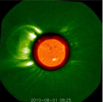
1.9 Observation of a CME and prominence lift-off from the EUVI and

COR1 instruments of the SECCHI suite on board the STEREO-A

spacecraft. The field-of-view extends to ∼4 R. The complexity

of the magnetic field driving the eruption is clearly indicated by

the twisted geometry of the bright ejecta.

Image credit: http://stereo.gsfc.nasa.gov/ . . . 24

1.10 Geometry of the Sweet-Parker (top) and Petschek (bottom)

recon-nection models, reproduced from Aschwanden (2005). . . 31

1.11 Illustrations of the different mechanical analogues of CME

erup-tions, reproduced from Klimchuk (2001). . . 34

1.12 Theoretical evolution of a 2D flux rope, reproduced from Forbes

& Priest (1995). The flux rope footpoint separation λ decreases,

increasing the magnetic pressure until the flux rope becomes

unsta-ble and erupts away from the surface (b – d). The resulting height

(15)

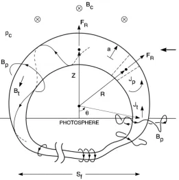
ent coronal magnetic fieldBcand plasma density ρc. Components

of the current density J and magnetic field B are shown, where

subscripts ‘t’ and ‘p’ refer to the toroidal and poloidal directions

respectively. The flux rope has a radius of curvatureR, radius of

cross-section a, apex height Z, footpoint separation sf, and the

radial force outward is FR. . . 39

1.14 Schematic, and corresponding simulation snapshots, of the main

stages of the axisymmetric 2.5D breakout model, reproduced from

Lynch et al. (2008). (a) shows the initial multipolar topology of

the system, (b) shows the shearing phase which distorts the X-line

and causes breakout reconnection to begin, (c) shows the onset

of flare reconnection behind the eruption that disconnects the flux

rope, and (d) shows the system restoring itself following the eruption. 42

1.15 The Thomson scattering geometry for a single electron, reproduced

from Howard & Tappin (2009). a) shows the electron and incident

light with different observer positions indicated. b), c), d) show

the resultant unpolarised, partially polarised, and polarised

scat-tering of light seen by observers O1, O2, O3 respectively. . . 45

1.16 Schematic of the Thomson surface, being the sphere of all points

which are located at an angle of 90◦ between the Sun and the

observer, reproduced from Vourlidas & Howard (2006). An

exam-ple line-of-sight is shown for an electron at point P, with radial

distancer from the Sun, at longitude φ relative to the solar limb. 47

1.17 (a) Synthetic coronagraph image of the model flux rope, deduced

from the integrated line-of-sight electron density, including a

con-sideration of the Thomson scattering geometry. (b) The flux rope

model represented by a mesh of helical field lines. Point A marks

the true apex of the model. The axes are in units of R.

(16)

1.18 Three example CME observations (off the limb, partial halo, and

full halo) and schematics showing how measurements of the

plane-of-sky velocityVP S and expansion velocityVexp are skewed by

pro-jection effects, reproduced from Schwennet al. (2005). . . 50

1.19 The CME velocity profile, and associated soft X-ray flare profile,

for the event on 11 June 1998, reproduced from Zhanget al.(2001).

The profiles indicate a three-phase scenario of CME evolution:

ini-tiation, impulsive acceleration, and propagation. The datapoints

are from LASCO/C1 (asterisks), C2 (triangles) and C3 (squares). 52

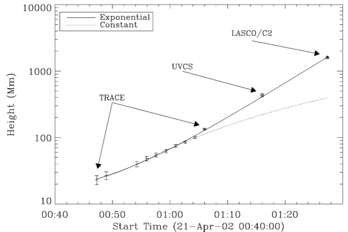
1.20 Height-time evolution of a CME observed with TRACE, UVCS

and LASCO/C2 on 21 April 2002, reproduced from Gallagheret al.

(2003). The datapoints have ±5 pixel errorbars, and the best fits

for an exponential varying and constant acceleration are plotted

for comparison. . . 53

1.21 (a) Height-time, (b) velocity and (c) acceleration profiles for the

CME on 21 April 2002, and (d) the GOES-10 soft X-ray flux for

the associated X1.5 flare during the interval 00:47 – 03:20 UT,

re-produced from Gallagher et al. (2003). A three-point difference

scheme is used on the data points, and a first-difference scheme is

plotted with filled circles. The solid line is the best fit of the

ex-ponentially increasing and decreasing acceleration of Equation 1.55. 54

1.22 The kinematics of the CME leading edge (circles), cavity (pluses)

and prominence (triangles) of the 15 May 2001 event, reproduced

from Mariˇci´cet al. (2004). (a) shows the height-time profiles. (b)

shows the distance between the leading edge and the prominence

(thick line), the cavity and the prominence (thin line), and the

leading edge and the cavity (dashed line). (c) shows the

veloci-ties determined by forward-difference technique upon the smoothed

height-times. (d) shows the onset of acceleration against height,

with a straight line fit. The horizontal bar between (a) and (c)

indicates the period of the soft X-ray burst (dotted- precursor,full

(17)

the hard X-ray flux of the associated flare (shown in red), peaking

simultaneously with the acceleration. . . 58

2.1 A schematic of the SOHO spacecraft and onboard instrument suites,

reproduced from Domingoet al. (1995). . . 63

2.2 The externally occulted Lyot coronagraph, reproduced from

Brueck-neret al.(1995), showing: front aperture A0 and external occulter

D1; entrance aperture A1 and objective lens O1; the field stop;

inner occulter D2 and field lens O2; Lyot stop A3 and relay lens

O3 with Lyot spot; filter and polariser wheels F/P; and the focal

plane F. . . 64

2.3 A LASCO/C3 image of the solar corona out to∼30 R. . . 65

2.4 Payload diagram of one of the STEREO spacecraft, indicating the

positions of the four instrument suites onboard: Sun-Earth

Con-nection Coronal and Heliospheric Imagers (SECCHI); In-situ

Mea-surements of Particles and CME Transients (IMPACT); Plasma

and SupraThermal Ion Composition (PLASTIC); STEREO/WAVES

radio burst tracker (SWAVES).

Image credit: stereo.gsfc.nasa.gov. . . 67

2.5 Diagram of the EUVI in the STEREO/SECCHI suite, reproduced

from Howard et al. (2000). . . 68

2.6 Diagram of the COR1 coronagraph in the STEREO/SECCHI suite,

reproduced from Howard et al. (2000). The measurements are

specified in millimetres. . . 70

2.7 Diagram of the COR2 coronagraph in the STEREO/SECCHI suite,

reproduced from Howard et al. (2000). The measurements are

specified in millimetres. . . 72

2.8 Diagram of the heliospheric imagers HI-1/2 in the STEREO/SECCHI

(18)

2.9 The intensity profile of a CME compared to the K & F coronae

observed at elongations up to 90◦, and the corresponding

fields-of-view of the Heliospheric Imagers (HI1/2), reproduced from Howard

et al. (2000). . . 74

2.10 Illustration of a thick front-side illuminated CCD.

Image credit: www.ing.iac.es. . . 75

2.11 Illustration of a thinned back-side illuminated CCD.

Image credit: www.ing.iac.es. . . 76

2.12 Schematics of two Sun-centred coordinate systems, reproduced

from Thompson (2006). (a) Stonyhurst heliographic coordinates

commonly used to locate features on-disk. (b) Heliocentric-cartesian

coordinates commonly used for spatially localising features in the

vicinity of the Sun. . . 79

2.13 Schematic of the celestial sphere and ecliptic plane. The celestial

equator is a projection of the Earth’s equator, and the ecliptic is

a projection of the Earth’s orbit about the Sun. . . 81

3.1 Raw (left) and pre-processed image (right) of a CME observed by

LASCO/C2 on 1 April 2004. The pre-processing includes

normalis-ing the image statistics, subtractnormalis-ing the background, and masknormalis-ing

the occulter disk. The white circle (right) indicates the relative

size and position of the Sun behind the occulter. . . 85

3.2 The top image (a) shows the detection of ridges in the (t, r) stacks

of the CACTus catalogue, through the use of the Hough transform

detailed in the bottom image (b), reproduced from Robbrecht &

(19)

black line distribution across the image represents the positive

value intensity count along each angle, and the two vertical black

lines mark the angular span at one standard deviation above the

mean intensity. (b) shows the new angular span following the

re-gion growing technique. (c) shows the intensity within the angular

span averaged across heights, and the ‘Half-Max-Lead’ is taken as

the CME height in the image. . . 90

3.4 An example of how the synoptic maps are generated for the ARTEMIS

catalogue, reproduced from Boursier et al. (2009b). At a chosen

height in the coronagraph image an annulus is unwrapped

(indi-cated with the dashed line and blue square, circle and triangle)

and these are then stacked together to illustrate how the intensity

at that height changes through time. Vertical streaks represent

transient events occurring on smaller time-scales than the more

persistent streamers in the images. . . 93

3.5 Top left, the horizontal detail, and top right, the vertical detail

from the high-pass filtering at one scale of the multiscale

decom-position (called the rows and columns respectively). Bottom left,

the corresponding magnitude (edge strength) and bottom right,

the angle information (0 – 360◦) taken from the gradient space, for

a CME observed in LASCO/C2 on 1 April 2004 (Byrneet al., 2009). 97

3.6 The vectors plotted represent the magnitude and angle determined

from the gradient space of the high-pass filtering at a particular

scale. The CME of 2004 April 1 shown here is highlighted very

effectively by this method (Byrne et al., 2009). . . 98

3.7 A normalised, background subtracted, LASCO/C2 image (left) of a

CME on 1 April 2004, and the resulting NRGF image (right). The

image radial intensity is scaled such that structure along streamers

(20)

3.8 A chosen scale of the decomposed NRGF image provides a

mag-nitude image of the edge strengths displayed on the left, which

is thresholded at one standard deviation from the mean intensity

to obtain contoured regions of interest that could contain a CME

(sample contours indicated in red). As shown, the streamers have

edges which appear on the same scale as the CME edges in this

image. The angular information from the decomposition is

dis-played on the right, and the contoured regions of interest overlaid

for comparison. The grey scale indicates angles from 0 – 360◦ and

it is clear that streamers tend to have a linear grey scale while the

CME has a gradient of greys across the scale. . . 103

3.9 Left: four contoured regions (at one standard deviation of the

mean image intensity) highlighted on the magnitude information

from the multiscale decomposition of the 1 April 2004 CME. Right:

the corresponding angular distribution of each region, normalised

and folded into the 0 – 180◦ range (centred on 90◦). The angular

distribution may be thresholded with respect to its median value

to distinguish regions corresponding to CMEs from those along

streamers. . . 104

3.10 The resulting CME detection mask from combining the

thresh-olded regions of strongest magnitude and angular distribution at

four scales of the decomposition. The 3D representation on the

right illustrates the pixel values of the mask. . . 105

3.11 The NRGF (left) and resulting detection masks (middle and right)

for different frames of a CME observed by LASCO/C2 at times

of 00:00 UT (top), 00:40 UT (middle) and 01:20 UT (bottom)

on 2 April 2004. The location of the CME front is highlighted

very efficiently by this method, although the detection masks may

contain artefacts of the chosen thresholds which must be discarded

(21)

image. (b) is the NRGF image. (c) and (d) show the magnitude

and angular information from the multiscale decomposition with

intensity contours overlaid in red. (e) and (f) show the resulting

CME detection mask in 2D and 3D respectively. . . 108

3.13 Ellipse tilted at angleδin the plane, with semimajor axisa,

semimi-nor axisb, and radial line ρ inclined at angle ω to the semimajor

axis. . . 110

3.14 A depiction of three frames sampled from the ellipse

characterisa-tion of a CME observed by LASCO/C2 on 24 January 2007. The

white dots along the CME front indicate the multiscale edge

de-tection to which the ellipse is fit. The black cross on the ellipse

indicates the furthest point measured from Sun centre which

pro-vides the height-time profile for determining the kinematics. The

opening angle from Sun centre measures the CME width. . . 112

4.1 A sample of ellipse fits to the multiscale edge detection of certain

events, reproduced from Byrne et al. (2009). For each event the

upper and lower image show LASCO/C2 and C3. . . 116

4.2 A sample of ellipse fits to the multiscale edge detection of certain

events, reproduced from Byrne et al. (2009). The two left event

images show LASCO/C2 and C3 in the upper and lower panels

respectively, while the two right events show SECCHI/COR1 and

COR2. . . 117

4.3 Kinematic and morphological profiles for the ellipse fit to the

mul-tiscale edge detection of the 2 January 2000 CME observed by

LASCO/C2 and C3. The plots from top to bottom are height,

velocity, angular width, and ellipse tilt. The CDAW heights are

over-plotted with a dashed line. The height and velocity fits are

(22)

multi-scale edge detection of the 18 April 2000 CME observed by LASCO/C2

and C3. The plots from top to bottom are height, velocity, angular

width, and ellipse tilt. The CDAW heights are over-plotted with

a dashed line. The height and velocity fits are based upon the

constant acceleration model. . . 126

(23)

bottom are height, velocity, angular width, and ellipse tilt. The

height and velocity fits are based upon the constant acceleration

model. . . 134

mul-tiscale edge detection of the 16 November 2007 CME observed by

SECCHI/COR1 and COR2 on STEREO-A. The plots from top to

bottom are height, velocity, angular width, and ellipse tilt. The

height and velocity fits are based upon the constant acceleration

model. . . 136

5.1 Schematic of the epipolar geometry used to relate the

observa-tions from the two STEREO spacecraft, reproduced from Inhester

(2006). This geometry enables us to localise features in 3D space

by the triangulating lines-of-sight across epipolar planes. . . 143

5.2 Schematic of how tie-pointing a curved surface within an epipolar

geometry is limited in its ability to resolve the true feature, since

lines-of-sight will be tangent to different edges of the surface and

not necessarily intersect upon it. Reproduced from Inhester (2006). 144

5.3 Schematic of the Graduated Cylindrical Shell (GCS) model of a

flux rope CME, reproduced from Thernisien et al. (2009).

Indi-cated are the model parameters of front height hf ront, leg height

h, angle between the legs 2α, cross-sectional radiusa, and distance

from Sun centreOto a point on the edge of the shell r. Two views

of the GCS model are shown; (a) ‘face-on’, and (b) ‘end-on’. The

positional parameters of longitude φ, latitude θ, and orientation

(24)

5.4 The elliptical tie-pointing technique developed to reconstruct the

3D CME front, shown here for the 12 December 2008 event. One of

any number of epipolar planes will intersect the ellipse

characteri-sation of the CME at two points in each image from STEREO-A

and B. (a) illustrates how the resulting four sight-lines intersect in

3D space to define a quadrilateral that constrains the CME front

in that plane. Inscribing an ellipse within the quadrilateral such

that it is tangent to each sight-line provides a slice through the

CME that matches the observations from each spacecraft. (b)

il-lustrates how a full reconstruction is achieved by stacking multiple

ellipses from the epipolar slices to create a model CME front that

is an optimum reconstruction of the true CME front. (c) illustrates

how this is repeated for every frame of the eruption to build the

reconstruction as a function of time and view the changes to the

CME front as it propagates in 3D. While the ellipse

characterisa-tion applies to both the leading edges and, when observable, the

flanks of the CME, only the outermost part of the reconstructed

front is shown here for clarity. . . 148

5.5 An ellipse inscribed within a convex quadrilateral. An isometry of

the plane is applied such that the quadrilateral has vertices (0,0),

(A, B), (0, C), (s, t). The ellipse has centre (h, k), semimajor axis

a, semiminor axisb, tilt angle δ, and is tangent to each side of the

quadrilateral. . . 149

5.6 The back-projection of a STEREO 3D CME front reconstruction

onto the SOHO/LASCO plane-of-sky, from the observations by

STEREO-A (red) and STEREO-B (green) at 16:22 UT on 26 April

(25)

STEREO-A. The right panel shows the running-difference

point-and-click ellipse characterisation of the CME front observed as

a halo event from STEREO-B. . The middle panel shows the

LASCO/C2 observation of the CME at 16:30 UT (8 minutes later

than the STEREO observations) with the back-projected 3D CME

front reconstruction overplotted for comparison. . . 154

5.8 Composite of STEREO-Ahead and Behind images from EUVI,

COR1, COR2, and HI1 (Byrne et al., 2010). (a) indicates the

STEREO spacecraft locations, separated by an angle of 86.7◦ at

the time of the event. (b) shows the prominence eruption observed

in EUVI-B off the NW limb from approximately 03:00 UT which

is considered to be the inner material of the CME. The

multi-scale edge detection and corresponding ellipse characterisation are

overplotted in COR1. (c) shows that the CME is Earth-directed,

being observed off the east limb in STEREO-A and the west limb

in STEREO-B. . . 155

5.9 STEREO-Ahead and Behind COR1 images at 07:35 UT on the 12

December 2008. Overplotted are: the multiscale edge detections of

the CME front (red); the ellipse characterisations (blue); and the

resulting 3D reconstructions back-projected onto the plane-of-sky

(white). . . 156

5.10 STEREO-Ahead and Behind COR2 images at 14:52 UT on the 12

December 2008. Overplotted are: the multiscale edge detections of

the CME front (red); the ellipse characterisations (blue); and the

resulting 3D reconstructions back-projected onto the plane-of-sky

(26)

5.11 STEREO-Ahead and Behind HI1 images at 01:29 UT on the 13

December 2008. Overplotted are: the running difference edge

detections of the CME front (red); the ellipse characterisations

(blue); and the resulting 3D reconstructions back-projected onto

the plane-of-sky (white). . . 158

5.12 The 3D CME front reconstruction as it propagates along the

Sun-Earth line through interplanetary space. This particular frame of

the reconstruction is from the observations of COR1 at 07:35 UT

on 12 December 2008. . . 159

the reconstruction is from the observations of COR2 at 14:52 UT

on 12 December 2008. . . 160

the reconstruction is from the observations of HI1 at 01:29 UT on

13 December 2008. . . 161

5.15 The graphical user interface for the 3D visualisation of the CME

front reconstruction, which may be used to change the orientation

of the observer, or the location of the definable parameters such as

time-stamps and distance measures (as displayed on the right). . . 162

5.16 The 3D CME front reconstruction from the COR2 Ahead and

Be-hind frames at 14:52 UT on 12 December 2008. The lines drawn

from Sun-centre indicate the ‘Midpoint of Front’ (solid blue), the

‘Northern / Southern Flanks’ (solid red / brown), and the

‘Mid-top / Midbottom of Front’ at angles in between (dashed red / brown).

By taking these measurements across all frames we may determine

the kinematics and morphology of the CME as plotted in

(27)

separation angle. . . 165

5.18 The kinematics of the prominence and 3D reconstructed CME

front of 12 December 2008. The prominence is observed as the

in-ner material of the CME, with both undergoing acceleration from

∼06:00 – 07:00 UT, peaking at ∼40 m s−2 _and _∼_{94 m s}−2

re-spectively, before reducing to scatter about zero. Measurement

uncertainties are indicated by one standard deviation error bars. . 168

5.19 Kinematic and morphological properties of the 3D reconstruction

of the 12 December 2008 CME front. The top panel shows the

velocity of the middle of the CME front with corresponding drag

model and, inset, the early acceleration peak. Measurement

uncer-tainties are indicated by one standard deviation error-bars. The

middle panel shows the declinations from the ecliptic (0◦) of an

angular spread across the front between the CME flanks with a

power-law fit indicative of non-radial propagation. The bottom

panel shows the angular width of the CME with a power-law

ex-pansion. . . 169

5.20 The 3D CME front parameters are used as initial conditions for an

ENLIL with Cone Model MHD simulation (Xie et al., 2004) and

the output density (top) and velocity (bottom) profiles of the inner

heliosphere are illustrated here for the time-stamp of 06:00 UT

on 14 December 2008. Beyond distances of ∼50 R the CME is

slowed by its interaction with the upstream, slow-speed, solar wind

flow along its trajectory towards Earth, and this accounts for its

arrival time as detected in-situ by the ACE and WIND spacecraft

(28)

5.21 The in-situ solar wind plasma and magnetic field data observed

by the WIND spacecraft. From top to bottom the panels show

proton density, bulk flow speed, proton temperature, and magnetic

field strength and components. The red dashed lines indicate the

arrival time of the density enhancement predicted from our ENLIL

with Cone Model run providing 08:09 UT on 16 December 2008,

with a potential offset error between our reconstruction and the

derived model height profiles accounting for an arrival time up to

13:20 UT. We observe a magnetic cloud signature behind the front,

as highlighted with blue dash-dotted lines. . . 175

5.22 Top: Ellipses characterising the 3D CME front reconstruction in

the out-of-ecliptic plane along the Sun-Earth line. Bottom: The

ellipse tilt angle is indicative of the initial effects of ‘pancaking’, as

the curvature of the CME front decreases with increasing height

(29)

to cycle through different scales, and threshold any number of

con-toured regions of magnitude (edge strength). Right: Contours that

contain a wide distribution of angles signal a CME detection. The

angular information is normalised to 1 and folded into a 0 – 180◦

range due to symmetry of the edge normals. A threshold on the

normalised angular distribution is specified to flag regions as CMEs

or otherwise (e.g.,>20%). A detection mask is then built through

multiple scales. The limitations to be overcome for a robust

au-tomation of this technique include developing dynamic thresholds

such that multiple contours of CME edges are not fragmented, and

increased angular distributions due to streamer deflections are not

mistakenly labelled as CMEs (a non-trivial task). Moreover, an

automated pixel chaining of the CME edges must be included in

order to produce an ellipse characterisation of the CME front in

the image. . . 189

6.2 An example interface which could be developed for the potentially

automated multiscale filtering and ellipse tracking of CMEs

ob-served by STEREO-A and B. Images from the respective

instru-ments appear on the left, and the resulting parameters from the

characterisation of the CME front appear on the right. Any

man-ner of information may be chosen for display, and clocked through

(30)

6.3 The magnitude (edge strength) from the multiscale filtering of a

CME observation, unwrapped into polar coordinates (r, θ) with

axis units of pixels and degrees, respectively. A scanning-line runs

over the image to produce the scatter of edge normals at the

bot-tom of the image, where each normal is plotted with a vector

mag-nitude and associated angular information from the multiscale

fil-ter (cf. the edge normals of Figure 3.6). An end-projection of

the normals along the scanning-line is plotted in the bottom right

of the image. The scanning-line is located at angle 328◦, passing

over a CME in the image. The resulting edge normals show a slice

through the angular distribution of the CME, and as the

scanning-line moves along the image, the end-projection shows a continuous

rotation of angles due to the curvature of the CME front.

Detect-ing this continuous rotation of angles may be used to distDetect-inguish

CMEs from streamers which show an abrupt, stepwise change in

angle as the scanning-line crosses over them. This may alleviate a

need for the intensity thresholding and contouring which can fail

to detect faint CMEs or portions thereof. . . 192

6.4 An example ridgelet, reproduced from Gallagheret al.(2010). The

first graph shows a typical ridgelet, and the second to fourth graphs

are obtained from simple geometrical manipulations, namely

rota-tion, rescaling and shifting. . . 194

6.5 The curvelet filtered image of a CME observed by LASCO/C2 on

18 April 2000, reproduced from Gallagheret al.(2010). The detail

along the curved CME front is enhanced as a result of the curvelet

technique following the removal of certain coefficients probably due

(31)

tions of CMEs are important for testing the validity of theoretical

models.

Image credit: http://www.nrl.navy.mil . . . 197

6.7 ‘Top’ view of the polarimetric reconstruction method applied to

both STEREO-A and B observations of a CME at 01:30 UT on the

31 December 2007 (rotated to the Sun-Earth frame), reproduced

from Moran et al. (2010). The red points are the reconstruction

from STEREO-A, and the blue points from STEREO-B, with the

green points showing the regions of overlap. . . 199

6.8 A theoretical model for a CME with constant acceleration 2 m s−2 and initial velocity 300 km s−1_{, and two simulations of how the}

resulting profiles for a noisy sample of datapoints behave using

3-point Lagrangian interpolation. . . 201

6.9 The resulting velocity profile for the 3D reconstructed CME front

of the 12 December 2008 using the inversion technique of Kontar

(32)

(33)

SEEDS and multiscale methods. Asterisks indicate analysis of

SECCHI data rather than LASCO. . . 122

4.2 Summary of CME accelerations as measured by CACTus, CDAW, SEEDS and multiscale methods. Asterisks indicate analysis of

SECCHI data rather than LASCO. . . 123

4.3 Summary of CME angular widths as measured by CACTus, CDAW,

SEEDS and multiscale methods. Asterisks indicate analysis of

(34)

(35)

The Sun, as provider of light and heat to all life on Earth, has been a

con-stant source of mystery and wonder to humankind. History recounts numerous

tales inspired by our connection with the Sun: from its worship as a deity in

the earliest civilisations, to the appreciation of its seasonal influence marked by

structures like Newgrange, and the eventual observance of its complex behaviour

with the development of telescopes and scientific intrigue. As our nearest star,

astronomers have increasingly taken interest in the complexities of the Sun, and

now in the modern age of space exploration numerous observatories have been

built specifically to monitor solar activity and further our understanding of its

(36)

1.1 The Solar Interior

The Sun is a G2V main sequence star of luminosity L = 3.85×1026 W, mass

M = 1.99×1030 kg and radiusR = 6.96×108 m (Prialnik, 2000). It was born from the gravitational collapse of a molecular cloud approximately 4.6×109 _years

ago, is currently in a state of hydrostatic equilibrium (∇P =−ρg), and predicted

to enter a red giant phase in another ∼5 billion years before ending its life as

a white dwarf (Phillips, 1999). Since we cannot directly observe the interior

of the Sun, its structure and evolution are fundamentally realised with the use

of the ‘standard solar model’ (SSM; Bahcall, 1989), which is a mathematical

treatment of stellar structure described by several differential equations derived

from basic physical principles. The SSM is constrained by the well-determined

boundary conditions of the Sun’s luminosity, radius, age and composition, and

thus provides a basis for understanding the mechanisms of energy transport in

the solar interior. It assumes hydrostatic equilibrium, with energy generated by

nuclear fusion, although small effects of contraction or expansion are included,

and any abundance changes are caused solely by the nuclear reactions. The

SSM is the end product of an iterative process that converges on an optimum

description of the internal energy generation and transport, and overall evolution

(37)

[image:37.595.114.527.180.577.2]

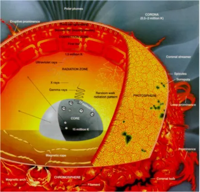
Figure 1.1: Illustration of the structure of the Sun. The core is the source of energy, where fusion heats the plasma to∼15 MK. Energy is transported from the core by radiative processes in the radiation zone. The convection zone is heated from the base at the tachocline, allowing convective currents to flow to the photo-sphere. Locations of strong magnetic fields inhibit convection and appear as dark sunspots on the photosphere. These strong magnetic fields extend into the upper atmosphere of the Sun, responsible for coronal loops, prominences and streamers.

(38)

The fundamental energy process driving the Sun is nuclear fusion in the core,

through the proton-proton chain at temperatures of∼15 MK:

1 1H +

1 1H →

2 1H + e

+₊_ν

e (1.1)

2 1H +

1 1H →

3

2He +γ (1.2)

3 2He +

3

2He → 4

2He + 2 1

1H (1.3)

where 1

1H is a proton, 21H is the deuteron isotope of hydrogen, 32He and 42He are

helium isotopes with 1 and 2 neutrons respectively, e+_{a positron,} _ν

e an

electron-neutrino and γ a gamma ray. The resulting energy release for one complete

reaction chain is approximately 4.3×10−12 _{J (Phillips, 1995). The core extends}

from the centre out to∼0.25 R, followed by the radiation zone out to∼0.75 R,

then the convection zone out to the solar surface at 1 R (Figure 1.1). The

temperature across the radiation zone drops to ∼5 MK with radiation being

the most efficient method of energy transport. This radiation field is closely

approximated by a black body, for which the spectral radiance is described by

the Planck equation:

Bλ(T) =

2hc2µ2

λ5_{[exp (}_hc/λkT₎₋_1] (1.4)

where Bλ(T) is the intensity of radiation per unit wavelength interval (at

tem-perature T), h is the Plank constant, c is the speed of light, µ is the

refrac-tive index of the medium, and k is the Boltzmann constant. By Wien’s law

λmaxT = 2.8979×10−3 m K we determine that the radiation is in the form of

(39)

es-elements move sufficiently rapidly for the energy interchange with their

surround-ings to be negligible, i.e., they change adiabatically. A useful measure of when

convection is likely to occur is given by the Schwarzschild criterion:

dlogT dlogP

star

> γ−1

γ (1.5)

where γ = CP/CV is the ratio of specific heats, equal to 5/3 for a perfect

monatomic gas. Essentially convection occurs once the absolute magnitude of

the radiative gradient becomes larger than the absolute magnitude of the

adi-abatic gradient, so that rising elements of plasma remain buoyant and move

towards the surface before they can lose heat to their surroundings. The rising

and falling parcels of plasma create the granulation effects observed on the

sur-face, with granules ranging in size from hundreds to thousands of kilometres and

dissipating over tens of minutes. (Details of the above radiative and convective

processes are found in, e.g., Kitchin (1987); Zirin (1998)).

Between the radiation and convection zones is a relatively thin interface called

the tachocline, where the solid body rotation of the radiative interior meets the

differentially rotating outer convection zone. It thus has a very large shear profile

which could account for the formation of large scale magnetic fields in the solar

dynamo. The magnetic field of the Sun has an overall dipolar configuration, with

opposite polarities dominant at each pole. The differential rotation of the Sun’s

(40)

Ω-effect, while the effects of the coriolis force and smaller scale motions of the

plasma can give twist and writhe to the field, named the α-effect (Figure 1.2).

Buoyancy effects cause the magnetic field to rise up through the convection zone

and protrude through the surface of the Sun, observed as sunspots on-disk

mark-ing the footpoints of over-archmark-ing concentrations of magnetic flux extendmark-ing up

through the solar atmosphere. In a given hemisphere one magnetic polarity leads

the sunspot group and the opposite follows, while in the opposite hemisphere

the situation is reversed (Hale’s law). The tilt angle between leading and

trail-ing sunspots has an average value of 5.6◦ relative to the E-W line (Joy’s law).

Furthermore, sunspots are observed to migrate from high latitudes towards the

equator over an 11 year cycle due to the continual build-up of field by the α

Ω-effect (Sp¨orer’s law). These combined effects lead to an increase of oppositely

oriented poloidal field at each of the poles, neutralising the field there and

re-sulting in the magnetic dipole flipping every 11 years. This 22 year periodicity

is known as the solar cycle, and gives rise to periods of increased and decreased

solar activity manifested by the frequency of phenomena such as active regions,

(41)

[image:41.595.256.379.138.319.2]

Figure 1.2: Illustration of theαΩ effect of winding-up magnetic field due to the differential rotation of the Sun, reproduced from Babcock (1961). Sunspots visible on the disk are as a result of protruding field with positivepand negativef polarity as shown.

1.2 The Solar Atmosphere

The Sun’s atmosphere is composed of all regions extending from the photosphere

out into the heliosphere. It may be separated into distinct regimes dependent

on the density and temperature profiles. These are plotted in Figure 1.3 for a

1D static model of the solar atmosphere. The layers are generally stratified into

photosphere, chromosphere, transition region, and corona; having a decreasing

density with increasing height from the photosphere, but from the chromosphere

up the temperature increases with a dramatic jump in the transition region giving

rise to the so-called ‘coronal heating problem’. However this stratification is a

simplified view and the solar atmosphere in reality is an inhomogenous mix of

photospheric, chromospheric and coronal zones due to complex dynamic processes

such as heated upflows, cooling downflows, intermittent heating, nonthermal

(42)

ab-sorption and scattering in cool plasma, acoustic waves, and shocks (Aschwanden,

2005). The interplay between the magnetic and gas pressure represents an

im-portant determining factor in the behaviour of structures throughout the solar

atmosphere, quantified by the plasma-β term:

β = pgas

pmag

= nkT

(B2_/₈_π₎ (1.6)

This is illustrated in Figure 1.4 for the different layers of the atmosphere. At

the photospheric level the plasma-β is large, and plasma motions dominate over

the magnetic field forces. Through the chromosphere and corona the plasma-β

decreases to low values where the magnetic field structures are seen to suspend

plasma in loops and filaments. Finally in the extended upper atmosphere the

plasma-β rises again, and the magnetic field is advected out with the solar wind

plasma flow to ultimately form the Parker spiral.

1.2.1 Photosphere

The surface of the Sun is the photosphere defined as the point where the optical

depth equals 2/3 for wavelengths of visible light, centred on 5,000 ˚A (τ5000 ∼2/3

for I/I0 = e−τ). The spectrum of light emitted has a profile like that of a black

body with an effective temperature of 5,800 K interspersed with the Fraunhofer

absorption lines due to the tenuous layers above the photosphere. It has a particle

density of∼1023 _m−3 _{and a thickness of less than 500 km. Cooler regions called}

sunspots have temperatures of 4,000 – 4,500 K and are due to intense magnetic

field activity that acts to suppress convective plasma motion. Granulation of the

(43)

Figure 1.3: A 1D static model of electron density Ne [cm−3] and temperature

Te [K] profiles in the solar atmosphere, reproduced from Gabriel & Mason (1982).

In the chromosphere, the plasma is only partially ionised. The plasma becomes fully ionized at the sharp transition from chromospheric to coronal temperatures.

zone below, with typical cell sizes on the order of 1,000 km in diameter. They

occur when hot plasma rises to the surface and is transported along it to the

granule edges, which appear darker as the plasma cools and descends. The gas

pressure dominates the magnetic pressure (β > 1), and the magnetic field is

effectively coupled to the plasma motion which sweeps it into the inter-granular

network.

1.2.2 Chromosphere

Above the photosphere lies the chromosphere where the temperature initially

drops to a minimum of∼4,500 K before increasing to∼20,000 K with increasing

(44)

0.0001 0.0010 0.0100 0.1000 1.0000 10.0000 100.0000 Plasma β (16πnkT/B2)

0.01 0.10 1.00 10.00 100.00 1000.00 10000.00

Height (Mm)

Photosphere Chromosphere Corona Solar Wind

Acceleration Region

β

> 1

β

> 1

β

< 1

Figure 1.4: Plasma β as a function of height for a regime of magnetic field strengths between∼100 and∼2,500 G, reproduced from Gary (2001). The dotted lines segregate the layers of photosphere (β >1), chromosphere and corona (β <1), and the solar wind (β >1).

density falls by a factor of almost a million from bottom to top, so the magnetic

field begins to dominate the chromospheric structure (β <1). The second law of

thermodynamics does not permit heating of the chromosphere with the thermal

energy of the cooler photosphere below. Biermann (1948), Schwarzschild (1948)

and Schatzman (1949) put forward ideas on the acoustic wave heating of the

chromosphere as a result of the convective plasma motions in the photosphere

and convection zone beneath. Referred to as the BSS model, the hypothesis is

that acoustic waves transport energy upward with little dissipation once the

ve-locity is below the sound speed. As the density drops and the veve-locity reaches

(45)

first introduced by Osterbrock (1961). An Alfv´en wave is a type of

magnetohy-drodynamic wave that propagates in the direction of the magnetic field with the

magnetic tension providing the restoring force and the ion mass density

provid-ing the inertia. In Alfv´en wave heating theories the magnetic field itself is thus

responsible for depositing energy from the subsurface into the chromosphere and

above. These theories better sit with observations of vigourous heating above

plages and emerging flux regions, since they imply the amount of heating is

pro-portional to the rate of magnetic change.

While the brightness of the photosphere overwhelms that of the chromosphere

in the optical continuum, the hotter chromospheric temperatures lead to the

hy-drogen being ionised, resulting in strong Hα emission. Filaments are observed

as dark channels on-disk in Hα images (called prominences when seen on the

limb). Numerous plasma columns called spicules are also observed on the limb,

that typically reach heights of ∼3,000 – 10,000 km above the Sun’s surface and

are very short-lived (rising and falling over ∼5 – 15 minutes).

Between the chromosphere and corona lies the transition region where the

temperature jumps rapidly to over 1 MK. It is only about 100 km thick and

it marks the point where magnetic forces dominate completely over gravity, gas

pressure and fluid motion (β 1). The extreme temperatures result in prominent

(46)

1.2.3 Corona

The outermost part of the solar atmosphere is the corona, with electron

den-sities ranging from ∼(1 – 2)×1014 _m−3 _{at its base height of} _∼_{2,500 km above}

the photosphere, to _.1012 m−3 for heights _&1 R above the photosphere (As-chwanden, 2005). The density varies across coronal holes which can have a base

density of ∼(0.5 – 1)×1014 _m−3_{, or across streamer regions with higher}

densi-ties of ∼(3 – 5)×1014 _m−3_{. Active regions that suspend and confine plasma in}

strong over-arching magnetic fields usually have the highest coronal densities of

∼2×1014_{– 2}_×₁₀15 _m−3_{. The temperature of the corona is generally} _&_{1 MK,}

as indicated by emission from highly ionised iron lines, for example, which again

appears to contradict the second law of thermodynamics given the much cooler

layers of the chromosphere and photosphere below (the ‘coronal heating

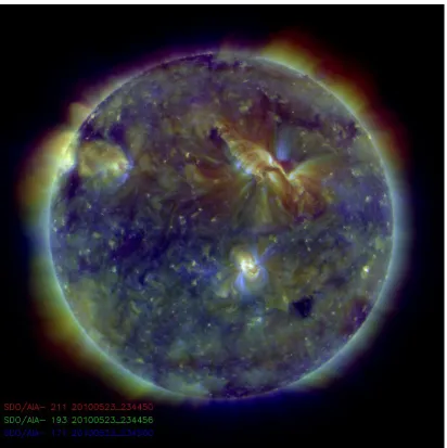
prob-lem’). Its temperature structure is far from homogeneous, revealed in images

such as that of Figure 1.5 from the Solar Dynamics Observatory (SDO). Loop

structures are observed at temperatures of 2 – 6 MK across regions of increased

magnetic field density (such as above active regions/sunspots), and closed field

regions are observed at temperatures of 1 – 2 MK across the quiet Sun, while

open field regions of coronal holes have temperatures _.1 MK. These high

tem-peratures lead to EUV and X-ray emission due to ionisation and recombination

processes from the interactions between photons, electrons, atoms and ions. The

continuum and line emission of the solar corona result from the contributions of

bound-bound transitions (excitations and de-excitations), bound-free absorption

(photoionisation), free-free absorption (and its inverse bremsstrahlung emission),

(47)

[image:47.595.115.528.196.610.2]

Figure 1.5: Composite EUV image of the low solar corona recorded by the Atmo-spheric Imaging Assembly (AIA) onboard the Solar Dynamics Observatory (SDO) on 23 May 2010.

(48)

produces the white-light corona as visible during a solar eclipse or with the use of

a coronagraph to occult the solar disk, which is six orders of magnitude brighter

in optical wavelengths.

The corona we observe comprises several parts:

• The K-corona has a strongly polarised continuous emission spectrum due to

Thomson scattering of photospheric light by the free electrons of the coronal

gas, and it dominates within the first few R. It produces a polarised

white-light continuum without the Fraunhofer lines which are broadened by

Doppler shifts due to the fast electron motions at such high temperatures.

The intensity of the K-corona gives the coronal electron density (Koutchmy

et al., 1991).

• The F-corona is due to scattering of sunlight by interplanetary dust

parti-cles, and contains the Fraunhofer lines. It is roughly equal in intensity to

the K-corona at ∼4 R, and dominates at greater distances.

• The E-corona is due to emission from highly ionized coronal atoms such as

iron and calcium.

• The T-corona is caused by thermal (infrared) emission of the interplanetary

dust. It is an unpolarised continuum, insignificant in the visible part of the

spectrum.

In contrast to the chromosphere, solar interior, and indeed the heliosphere, the

magnetic pressure in the corona dominates over the gas pressure and so governs

the coronal plasma dynamics (β < 1). The coronal structure we observe is thus

(49)

greatly over the solar activity cycle: it appears rounder at solar maximum, when

multiple streamers emerge at various latitudes distributed across the Sun; and it

appears more elliptical at solar minimum, when only a few streamers are present,

lying closer to the equator.

Following Chapman & Zirin (1957) the description of a static corona leads

to an unreasonable pressure value at large distances from the Sun. This is

out-lined below, beginning with the assumption that the corona is in hydrostatic

equilibrium:

dP

dr = −ρ

GM

r2 (1.7)

The plasma density is ρ=nmp, the pressure contribution from the protons and

electrons is P = 2nkBT, and the coronal heat flux is q = κ∇T with thermal

conductivity κ =κ0T5/2. In the absence of heat sources or sinks∇ ·q = 0 so in

a spherically symmetric system we can write:

1

r2

d dr

r2κ0T5/2

dT dr

= 0 (1.8)

Applying the boundary condition that the temperature tends to zero at large

distances from the Sun, we obtain:

T = T0

r₀

r

2/7

(50)

where T0 = 2 MK is the temperature of the low corona at height r0 = 1.05 R from Sun centre. This would mean T ≈ 4×105 K at Earth (1 AU≈215 R), close to measured values. Rewriting in terms of pressure and integrating, results

in:

P(r) = P0exp

7 5

GMmp

2kT0r0

r_o

r

5/7 −1

(1.10)

which implies that asr→ ∞the coronal pressure tends towards a finite constant

value significantly larger than the pressure of the interstellar medium (ISM);

P PISM. This means the static coronal model is unphysical, and a dynamic

model in which the material flows outward from the Sun must be considered,

leading to a description of the solar wind.

1.2.4 Solar Wind

The solar wind is the constant out-stream of charged particles of plasma from

the Sun’s atmosphere due to the persistent expansion of the solar corona. The

wind consists mostly of electrons and protons at energies of ∼1 keV, observed

in two regimes of propagation: the slow solar wind with speeds of ∼400 km s−1_;

and the fast solar wind with speeds of ∼800 km s−1_{, originating from regions of}

open magnetic field such as coronal holes. Thermal velocities of the particles are

calculated at ∼260 km s−1 for coronal temperatures on the order of 3×106 _K,

while the escape velocity in the Sun’s gravitational field in the low corona can

be ∼500 km s−1_{. The additional energy to accelerate the solar wind is imparted}

by the pressure gradient PSun PISM to attain the measured solar wind speeds

(Parker, 1958). The Parker model assumes the outflow is steady, spherically

(51)

V

IV

II

r/r

v/v

c c

0 1 2 3 4 5 6 2

1

0

I

III

Figure 1.6: The five classes of Parker’s solar wind solution for a steady, spherically symmetric, isothermal outflow.

takes the form:

ρvdv

dr = −

dP dr −ρ

GM

r2 (1.11)

Considering mass conservation ˙m= 4πr2_ρv ₌_constant_{, we obtain:}

∂ ∂r r

2_ρv

= 0 ⇒ 1

ρ ∂ρ

∂r = −

1 v ∂v ∂r − 2 r (1.12)

So for a perfect gasP =RρT Equation 1.11 can be written:

v−RT

v ∂v ∂r − 2RT r + GM

(52)

A critical point occurs when∂rv →0 so we define:

rc =

GM

2v2

c

where vc =

√

RT (1.14)

and rewrite Equation 1.13 as:

v2−v2_c 1

v ∂v

∂r = 2

v2

c

r2 (r−rc) (1.15)

Integrating Equation 1.15 gives Parker’s ‘solar wind solutions’:

v vc 2 −ln v vc 2

= 4 ln

r rc

+ 4rc

r +C (1.16)

whereC is a constant of integration, leading to five potential solutions as plotted

in Figure 1.6. Solutions I and II are double-valued, with II being disconnected

from the surface. Solution III is too large (supersonic) close to the Sun.

So-lution IV is called the ‘solar breeze’ as it remains subsonic. SoSo-lution V is the

standard solar wind solution, although the assumptions of radial expansion and

isothermality are not completely true in reality, so it is only an approximate

characterisation of the observed solar wind. Nonetheless it is sufficient to convey

the dynamic expansion of the corona and ultimate supersonic regime of outflow,

often described akin to a de Laval nozzle which is used to accelerate flows from

subsonic to supersonic speeds (as detailed in Goossens, 2003, for example). The

presence of the solar wind was confirmed in 1959 by the Lunik I probe, and in

1962 by the Mariner II mission en route to Venus (Neugebauer & Snyder, 1962).

(53)

at-Figure 1.7: Schematic of the Parker Spiral in the heliosphere. The streamlines of the solar wind act to drag out the magnetic field lines of the Sun, which become wound up in an Archimedean spiral as a result of the Sun’s rotation.

Image credit: Steve Suess, NASA/MSFC.

mosphere (β > 1), the solar wind acts to drag out the magnetic field lines of

the Sun which become wound up as a result of solar rotation to form the Parker

Spiral (Figure 1.7). This is an Archimedean spiral drawn by the magnetic field

lines as they are advected outward by the solar wind, described by the equation:

r−r0 =

v

Ω(θ−θ0) (1.17)

where θ is the polar angle, Ω = 2.7×10−6 _{rad s}−1 _{is the angular rotation rate}

of the Sun, r is the distance, and v is the solar wind speed (Parks, 2004; Zirin,

[image:53.595.168.475.147.423.2]

(54)

interaction regions (CIRs) where the fast wind encounters the slow wind ahead

of it in the Parker spiral, and can form shocks in the solar wind.

The solar wind does not extend infinitely, but eventually terminates when it

reaches the edge of the heliosphere. The point where the solar wind slows from

supersonic to subsonic speeds is called the termination shock, the observation of

which is reported in a series of papers discussing the data from Voyager II as

it began to cross the shock in August 2007 (Burlaga et al., 2008; Decker et al.,

2008; Richardson et al., 2008). Beyond the termination shock, the wind comes

into pressure balance with the ISM to form the heliosheath, whose outer boundary

is called the heliopause (Figure 1.7). In the heliosheath the continually slowing

wind is compressed and becomes turbulent through its interaction with the ISM

(Opheret al., 2009). As the heliosphere moves through interstellar space, a bow

shock is thought to form ahead of the heliopause as it encounters the ISM.

1.2.5 Space Weather

Space weather is the name attributed to phenomena involving ambient plasma,

magnetic field, radiation and other matter affecting the conditions in space as

part of the vast field of heliophysics (Schrijver & Siscoe, 2010). It is

predom-inantly due to the influences of the solar wind, flares and transients, and the

interplanetary magnetic field (IMF). Earth’s magnetosphere provides a natural

shielding of the planet from the solar wind and space radiation, although large

flares and coronal mass ejections (CMEs) that accelerate solar energetic particles

(SEPs) can lead to geomagnetic storms at Earth which perturb the

(55)

[image:55.595.115.525.139.405.2]

Figure 1.8: The Aurora Borealis, or Northern Lights, photographed above Bear Lake, Eielson Air Force Base, Alaska. Aurorae result from photon emissions of excited oxygen and nitrogen atoms in the Earth’s upper atmosphere, as a result of geomagnetic storms and space weather.

Image credit: Joshua Strang via Wikimedia Commons.

throughout history are an indicator of geomagnetic storm occurrences (e.g.,

Fig-ure 1.8), and by 1837 they were realised to be caused by electric currents in

the upper atmosphere (Olmstead, 1837). Sabine (1852) went on to show that

there was a detailed correlation between the sunspot cycle and the frequency

of auroral displays, implicating solar activity as the ultimate cause of the

auro-ral phenomenon. A key event in the realisation of how strongly solar activity

can influence us on Earth, was the Carrington-Hodgson flare that occurred on

1 September 1859 (Carrington, 1859), causing widespread sightings of aurorae

down to latitudes as low as ∼18◦ and the loss of a significant portion of the

(56)

comprises the ejection of two CMEs from the Sun on 27 August and 1 September

1859, whose interaction as the second CME ploughs through the first produced

a shock responsible for the extreme nature of the 2 – 3 September auroral event

(Green & Boardsen, 2006). More recently, a severe geomagnetic storm on 13

March 1989 caused the collapse of the Hydro-Qu´ebec power network due to a

transformer failure from the geomagnetically induced currents (GIC). Six million

people were left without power for nine hours, with a substantial economic loss.

The cause was a CME ejected from the Sun on 9 March 1989 impacting the Earth

several days later. Other CMEs have similarly knocked out communication

satel-lites such as the Canadian Aniks E1 and E2 and the international Intelsat K on

20 January 1994, and the AT&T Telstar 401 on 7 January 1997. Moreover, the

increased radiation of solar and space weather storms poses a risk to astronauts

and high-altitude flight passengers, particularly when travelling over the poles. In

the modern era of technological advancement and increased dependency on

satel-lites communications, GPS networks and power distribution grids, the influence

of space weather is an increasing cause for concern. A recent report by the US

National Research Council (Committee On The Societal & Economic Impacts Of

Severe Space Weather Events, 2008) indicates that the potential economic cost of

a high-level geomagnetic storm could be up to $2 trillion. Thus the monitoring

and forecasting of potentially hazardous events is of great importance to society

at large, with particular emphasis on CMEs and the dynamics governing their