Analysis of Effect of Oblateness of Smaller Primary on the Evolution of Periodic Orbits

http://www.scirp.org/journal/ijaa ISSN Online: 2161-4725 ISSN Print: 2161-4717

Analysis of Effect of Oblateness of Smaller

Primary on the Evolution of Periodic Orbits

Niraj Pathak

, V. O. Thomas

1_{Department of Mathematics, Dharmsinh Desai University, Nadiad, India}

2_{Department of Mathematics, The Maharaja Sayajirao University of Baroda, Vadodara, India}

Abstract

Evolution of periodic orbits in Sun-Mars and Sun-Earth systems are analyzed using Poincare surface of section technique and the effects of oblateness of smaller primary on these orbits are considered. It is observed that oblateness of smaller primary has substantial effect on period, orbit’s shape, size and their position in the phase space. Since these orbits can be used for the design of low energy transfer trajectories, so perturbations due to planetary oblateness has to be understood and should be taken care of during trajectory design. In this paper, detailed stability analysis of periodic orbit having three loops is given for A2 = 0.0001.

Keywords

Restricted Three Body Problem, Low Energy Trajectory Design, Periodic Orbits, Oblateness, Poincare Surface of Section

1. Introduction

A low-energy transfer trajectory [1] is a trajectory in space that allows spacecraft to change the existing orbits using very small amount of fuel in comparison with Hohmann transfer orbit. To construct low-energy transfer trajectories, we require periodic orbits of spacecrafts around both primary bodies. Space agencies are trying to place telescopes into deep space like NASA’s Terrestrial Planet Finder and ESA’s Darwin project, to find Earth-like planets around other stars exhibiting life. In order to make space mission to explore different aspects of far away objects, it is required to determine special types of orbits that cannot be found by classical approaches.

However, it is to be noted that the classical approaches to spacecraft design are like Hohmann transfer for Apollo Moon landings and swing bys of outer planets for voya-ger. But these missions were costly in terms of fuel. A very high fuel requirement for How to cite this paper: Pathak, N. and

Thomas, V.O. (2016) Analysis of Effect of Oblateness of Smaller Primary on the Evo-lution of Periodic Orbits. International Journal of Astronomy and Astrophysics, 6, 440-463.

http://dx.doi.org/10.4236/ijaa.2016.64036

Received: November 13, 2016 Accepted: December 24, 2016 Published: December 27, 2016

Copyright © 2016 by authors and Scientific Research Publishing Inc. This work is licensed under the Creative Commons Attribution International License (CC BY 4.0).

the Sun and Earth, or the Sun and Mars, or any other pair of heavenly bodies that can produce considerable gravitational field. We take the total mass of the primaries nor-malized to 1. Mass of bigger primary is taken as 1 − μ and that of smaller primary is μ. The two main bodies rotate in the plane in circular orbits counter clockwise about their common center of mass and with angular velocity which is also normalized to 1. The third body, the spacecraft, has an infinitesimal mass and is free to move in the plane. Generalization to the 3-dimensional problem is of course important, but many of the essential dynamics can be captured well with the planar model. [1] studied low energy transfer to the Moon. In this study, they considered four bodies Sun-Earth-Moon- Spacecraft as coupled three body systems, namely Sun-Earth-spacecraft and Earth-Moon- spacecraft. They constructed low energy transfer trajectories from the earth which ex-ecuted ballistic capture at the Moon.

[3] is a fundamental book on the RTBP. Because of the non-linear nature of the equ-ations of motion involved in the study of the system, analytical methods may not give illuminating insights into the solution. So, Poincare surface of section (PSS) is widely used for finding the orbits of the infinitesimal particle (spacecraft) and analyzing peri-odic, quasi periodic and chaotic orbits. Solar system dynamics by [4] provide a detailed analysis of periodic orbits using PSS technique.

the smaller primary an oblate body. [14] computed series of horizontally critical sym-metric periodic orbits of the six basic families of the restricted three-body problem when the more massive primary is an oblate spheroid. The vertical stability of the hori-zontally critical orbits is also computed.

A large number of periodic orbits were generated by [15] in the framework of RTBP numerically. He classified the orbits into ten families. His work widely referred in lite-rature. These studies explore the regions of the phase space that contain sensitive de-pendence on initial conditions. [16][17] and [18] made extensive study on phase space by exploring large portion of the phase plane with Poincare surfaces of section (PSS)

[19]. This technique was also used by [20][21][22] and [23] to explore the phase space of a system with the Sun-Jupiter mass ratio.

Recently, [24] analyzed Sun and Saturn centered periodic orbits with solar radiation pressure and oblateness and found that there is a substantial effect of solar radiation pressure on position and geometry of infinitesimal particle orbit. [25] had studied fam-ily “f” orbits and their stability for Sun-Saturn system with perturbation. In their study Sun was taken as a source of radiation and Saturn was considered as oblate spheroid. By taking the actual coefficient of oblateness for Saturn and different values of solar radia-tion pressure, the family “f” orbits have been analyzed in detail.

Periodic orbits of spacecraft around two primaries are used to construct low energy trajectory. [26] established three classes with orbits around both primaries depending on motion of spacecraft is prograde or retrograde in the rotating system as well as fixed system. In this paper we have analyzed periodic orbits around both primaries with re-trograde motion in rotating system and analyzed periodic orbits having number of loops from 1 to 5 for different pairs of oblateness coefficient A2 and Jacobi constant C

for Sun-Mars and Sun-Earth system. It has been found that A2 and C has substantial

effect on the position in phase space, shape and size of the orbits and hence must be considered during low energy trajectory design.

2. Equations of Motion

Let m1 and m2 be two masses of first primary and second primary bodies. Mass of first

primary is greater than mass of second primary. The perturbed mean motion n of second primary body is given by,

2

2 3

1 ,

2

n = + A (1)

where

2 2

2 2 .

5

e p

A

R

ρ −ρ

= ₍₂₎

Here A2 is oblateness coefficient of second primary. ρe and ρp represent equatorial

sys-where

(

)

(

)

2

2 2 2

1 2 3

1 2 2

1 1 . 2 2 A n r r

r r r

µ µ µ

µ µ −

 

Ω = _ − + _+ + + ₍₄₎

Here

(

)

2 2

1 ,

r = x−µ +y (5)

and

(

)

2 2

2 1 .

r = x+ −µ +y (6)

Equations (3) and (4) lead to the first integral

2 2

2 ,

x +y = Ω −C (7)

where C is Jacobi constant of integration given by

(

)

(

)

(

)

2 2 2 2 2

1 2 3

1 2 2

1

1 2 2 A .

C n r r y

r r r

µ µ µ

µ µ

= − + + − + + −  (8)

These equations of motion are integrated in (x, y) variables using a Runge-Kutta Gill fourth order variable or fixed step-size integrator. The initial conditions are selected along the x-axis. By defining a plane, say y = 0, in the resulting three dimensional space the values of x and x can be plotted every time the particle has y = 0, whenever the trajectory intersects the plane in a particular direction, say y > 0. We have constructed Poincare surface section (PSS) on the x, x plane. The initial values were selected along the Ox-axis by using intervals of length 0.001. By giving different value of C we can plot the trajectories, and then analysis of orbits can be done.

3. Results and Discussion

We shall consider two systems, the Sun-Mars system and the Sun-Earth system. The mass of Sun, Earth and Mars considered in the study are 1.9881 × 1030 _{kg, 5.972 × 10}24

kg and 6.4185 × 1023 _{kg, respectively, [5]. Thus, for the Sun-Earth and Sun-Mars}

sys-tems, mass factor μ are 0.000003002 and 0.0000003212 respectively. Equatorial and po-lar radii of Earth are 6378.1 kms. and 6356.8 kms. and that of Mars are 3396.2 kms. and 3376.2 kms., respectively. The distance between Sun and Earth is taken as 149,600,000 kms. and distance between Sun and Mars is 227,940,000 kms. So, oblateness coefficient calculated from Equation (2) for Sun-Earth and Sun-Mars have values A2 = 2.42405 ×

10−12 _{and A}

neg-ligible, they definitely affect orbits with close proximity. In order to study the effect of oblateness on periodic orbit around both primaries, we take different values of oblate-ness that can make observable changes in different parameters. For a given A2, selection

of C is not arbitrary. By solving Equation (8) w.r.t. 2

x and by setting in to this equa-tion y = 0 and 2

y > 0 the resulting inequality defines the regions allowed to motion on the PSSs. Thus, we eliminate the possibility of excluded region for secondary body between Sun and Earth (or Mars). This maximum value of C is considered as admissi-ble value of C.

Table 1 and Table 2 show range of admissible values of C for Sun-Mars and Sun- Earth systems. It can be observed that for both systems as oblateness increases, admiss-ible range of C increases. But this increment is larger for Sun-Earth system than Sun- Mars system. So, we can say that as mass factor increases, effect of oblateness increases and due to that admissible range of C increases.

We have studied the effect of oblateness on the location and period of Sun-Mars sys-tem for different values of Jacobi constant C using PSS. Figure 1 is PSS constructed for Sun-Mars system when (A2, C) is (0.0005, 2.93) by taking value of x from the interval

[0.8, 1] with interval of x differencing as 0.001. Also, time span t = 10,000 time units and interval of time differencing is taken as 0.001. So, for each x equations of motions are integrated using Runge-Kutta-Gill method. Each solution is plotted as a point in

Figure 1. The arcs of PSS are known as islands whose center gives periodic orbit. In a similar way, we can obtain PSS for Sun-Earth which is shown in Figure 2. This PSS is also constructed for the pair (A2, C) given by (0.0005, 2.93). Our aim is to make a

comparative study of the effect of oblateness on different parameters of the orbits of Sun-Earth and Sun-Mars systems using PSS technique. Mass factor μ of Sun-Earth is greater than Sun-Mars.

For Sun-Mars system, the numerical values of location of periodic orbit and left end

Table 1. Admissible range of C for Sun-Mars system.

A2 Maximum value _{of C greater than maximum value} Value of C _(where Excluded region _{y is complex) excluded region} Size of

0.00001 3.00 3.001 0.984 to 0.999 0.016 0.00005 3.00 3.001 0.984 to 0.998 0.015 0.0001 3.00 3.001 0.985 to 0.997 0.013 0.0005 3.001 3.002 0.981 to 0.995 0.015

Table 2. Admissible range of C for Sun-Earth system.

A2 Maximum value _{of C greater than maximum value} Value of C _(where Excluded region _{y is complex) excluded region} Size of

Figure 1. PSS for A2 = 0.0005 and C = 2.93, for x = [0.8, 1], t = 10,000 for Sun-Mars system.

Figure 2. PSS for A2 = 0.0005 and C = 2.93, for x = [0.8, 1], t = 10,000 for Sun-Earth system.

(L) and right end (R) of corresponding island for C = 2.93, 2.94, 2.95, 2.96 and for ob-lateness A2 = 0.00001, 0.00005, 0.0001 and 0.0005 are displayed in Table 3. It is

ob-served from the table that a change in C in the range (2.93, 2.96) affects the location of the periodic orbits. Oblateness also affects the location of the periodic orbit. Similarly, the effects of C and A2 in the location of periodic orbits and left end (L) and right end

(R) of corresponding island for the Sun-Earth system are studied and the numerical es-timates of the changes are displayed in Table 4. Size of the island gives stability of the corresponding orbit.

The periodic orbits starting from single-loop to five loops in the Sun-Mars and Sun-Earth systems for A2 = 0.0005 and C = 2.93 are shown in Figures 3(a)-(j). It can be

Table 3. Analysis of periodic orbit for different pairs of A2 and C for Sun-Mars system.

NO. OF LOOPS C A2 = 0.00001 A2 = 0.00005 A2 = 0.0001 A2 = 0.0005

Location (x) L R Location (x) L R Location (x) L R Location (x) L R

1

2.96 0.98295 0.9829 0.983 0.98285 0.9827 0.983 0.98272 0.9825 0.9829 0.9816 0.9815 0.9817 2.95 0.9679 0.9678 0.968 0.9678 0.9676 0.968 0.96765 0.9669 0.9686 0.9666 0.966 0.967 2.94 0.95324 0.953 0.9535 0.95314 0.953 0.9533 0.953 0.953 0.953 0.95196 0.9519 0.952 2.93 0.93896 0.9389 0.939 0.93887 0.9387 0.939 0.93875 0.9386 0.9389 0.93772 0.9376 0.9378

2

2.96 0.94149 0.9406 0.9425 0.94136 0.9411 0.9414 0.94119 0.941 0.9414 0.93985 0.9397 0.94 2.95 0.92251 0.9224 0.9226 0.92239 0.9223 0.9225 0.92223 0.922 0.9225 0.92096 0.9209 0.921 2.94 0.9045 0.9042 0.905 0.90438 0.9041 0.905 0.90424 0.904 0.9045 0.90302 0.903 0.903 2.93 0.88734 0.887 0.8878 0.88722 0.887 0.8874 0.88708 0.887 0.8872 0.88592 0.8858 0.886

3

2.96 0.91529 0.915 0.9156 0.91514 0.915 0.9153 0.91496 0.9149 0.915 0.91348 0.9133 0.9137 2.95 0.89425 0.894 0.8945 0.89412 0.894 0.8942 0.89395 0.8939 0.894 0.89258 0.8922 0.893 2.94 0.87463 0.8743 0.8748 0.87449 0.8743 0.8747 0.87433 0.874 0.8747 0.87305 0.873 0.8731 2.93 0.85616 0.856 0.8563 0.85604 0.856 0.8561 0.85588 0.8558 0.856 0.85467 0.8543 0.855

4

2.96 0.89703 0.897 0.8971 0.89688 0.8968 0.897 0.89668 0.8965 0.8969 0.89515 0.895 0.8953 2.95 0.8749 0.8748 0.875 0.87476 0.8745 0.875 0.87458 0.874 0.875 0.87316 0.873 0.8733 2.94 0.85447 0.8544 0.8545 0.85433 0.854 0.8547 0.85417 0.8541 0.8543 0.85284 0.8527 0.853 2.93 0.8354 0.835 0.836 0.83528 0.835 0.8357 0.83512 0.835 0.8353 0.83388 0.8338 0.834

5

2.96 0.88363 0.8832 0.8834 0.88347 0.883 0.8838 0.88328 0.883 0.8836 0.8817 0.8814 0.882 2.95 0.8609 0.8608 0.861 0.86075 0.8605 0.861 0.86057 0.8602 0.8609 0.85912 0.859 0.8593 2.94 0.84004 0.84 0.8401 0.83991 0.8398 0.84 0.83974 0.8394 0.8401 0.83839 0.8383 0.8385 2.93 0.82068 0.8204 0.821 0.82056 0.8205 0.8206 0.8204 0.82 0.8208 0.81914 0.819 0.8193

Table 4. Analysis of periodic orbit for different pairs of A2 and C for Sun-Earth system.

NO. OF LOOPS C A2 = 0.00001 A2 = 0.00005 A2 = 0.0001 A2 = 0.0005

Location (x) L R Location (x) L R Location (x) L R Location (x) L R

1

2.96 0.983 0.983 0.983 0.9829 0.9828 0.983 0.9828 0.9828 0.9828 0.9817 0.9817 0.9817 2.95 0.9679 0.9678 0.968 0.96782 0.9676 0.968 0.9677 0.9674 0.968 0.9666 0.9662 0.967 2.94 0.95325 0.953 0.9535 0.95315 0.953 0.9533 0.95304 0.9530 0.9531 0.952 0.952 0.952 2.93 0.939 0.939 0.939 0.9389 0.9388 0.939 0.93877 0.9385 0.939 0.93775 0.9375 0.938

2

2.96 0.94155 0.941 0.942 0.9414 0.941 0.9418 0.94125 0.941 0.9415 0.9399 0.9398 0.94 2.95 0.92255 0.9221 0.923 0.92244 0.922 0.923 0.92226 0.922 0.9225 0.921 0.921 0.921 2.94 0.90455 0.904 0.9051 0.90442 0.904 0.9048 0.90426 0.904 0.9045 0.90305 0.903 0.9031 2.93 0.88737 0.887 0.8877 0.88725 0.887 0.8875 0.8871 0.887 0.8872 0.88595 0.8859 0.886

3

2.96 0.91535 0.915 0.9157 0.9152 0.915 0.9154 0.915 0.915 0.915 0.91354 0.9131 0.9141 2.95 0.8943 0.894 0.8946 0.89416 0.894 0.8943 0.894 0.894 0.894 0.89262 0.8922 0.893 2.94 0.87465 0.8743 0.875 0.87453 0.8741 0.875 0.87438 0.874 0.8748 0.87309 0.873 0.8732 2.93 0.8562 0.8554 0.857 0.85608 0.856 0.8562 0.85592 0.8558 0.856 0.8547 0.8544 0.855

4

2.96 0.8971 0.897 0.8972 0.89695 0.8969 0.897 0.89675 0.8965 0.897 0.8952 0.895 0.8954 2.95 0.87495 0.8749 0.875 0.87482 0.8746 0.875 0.87464 0.8743 0.875 0.87321 0.873 0.8734 2.94 0.8545 0.854 0.855 0.85438 0.854 0.8548 0.85421 0.854 0.8544 0.85289 0.8528 0.853 2.93 0.83544 0.835 0.8359 0.83532 0.835 0.8356 0.83516 0.835 0.8353 0.83392 0.8338 0.834

5

(a) Sun-Mars system C = 2.93, A2 = 0.0005, period 13. (b) Sun-Earth system C = 2.93, A2 = 0.0005, period 13.

(c) Sun-Mars system C = 2.93, A2 = 0.0005, period 19. (d) Sun-Earth system C = 2.93, A2 = 0.0005, period 19.

(e) Sun-Mars system C = 2.93, A2 = 0.0005, period 26. (f) Sun-Earth system C = 2.93, A2 = 0.0005, period 26.

(i) Sun-Mars system C = 2.93, A2 = 0.0005, period 38. (j) Sun-Earth system C = 2.93, A2 = 0.0005, period 38. Figure 3. Periodic orbits around both primaries for Sun-Mars and Sun-Earth systems.

around the second primary (Mars or Earth) in addition to orbiting both primaries. Further the secondary body is closest to Mars or Earth in the single-loop closed orbit. Such orbits may be useful in the study of different aspects of both primaries. In many models available in literature not many closed orbits possess this kind of nature. Fur-ther the position of the orbit in the case of odd number of loops approaches the first primary, namely the Sun. This is true in the case of even number of loops also. It can be observed that the period of the orbit remains unchanged due to change in oblateness or mass factor, but period of the orbit increases with increment in number of loops.

We have studied the variation of position of periodic orbits around Sun-Mars and Sun-Earth system due to the variation in oblateness and Jacobi constants C. In Figure 4

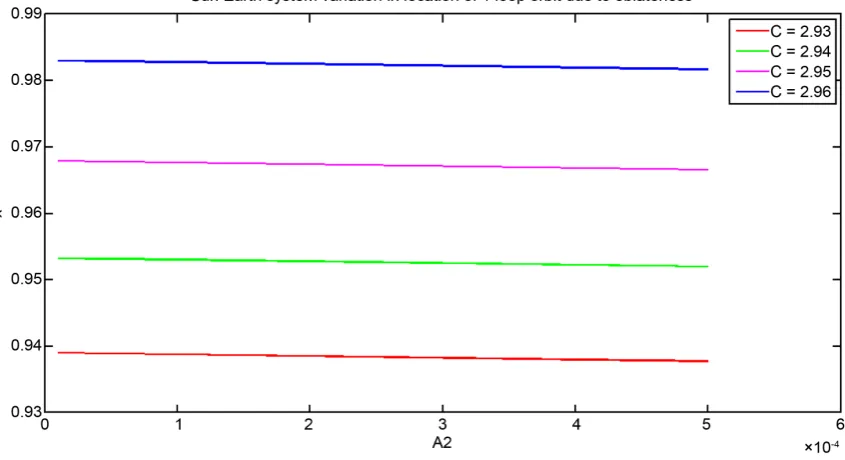
we have shown the variation of position of closed periodic orbit with single-loop for oblateness in the range (0, 0.0005) for Sun-Mars system corresponding to Jacobi con-stants C = 2.93, 2.94, 2.95 and 2.96. From Figure 5 it is clear that the position of the or-bits recedes away from Mars when the oblateness increases and C decreases.

Similar kind of conclusion can be drawn from Figure 5 for the Sun-Earth system. We have studied the effect of A2 and C on the position of the orbits having loops

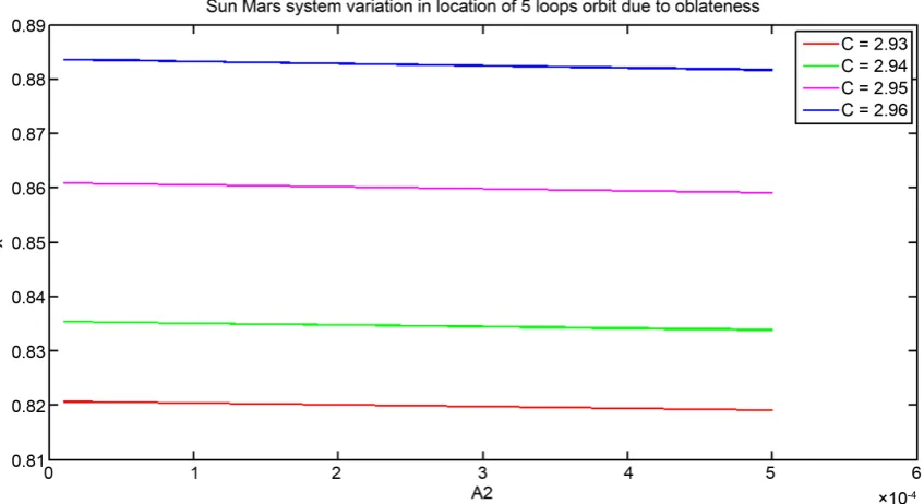
va-rying from 1 to 5 for both Sun-Mars and Sun-Earth systems. The results of these ob-servations for 5 loops closed periodic orbit in both Sun-Mars and Sun-Earth systems are shown in Figure 6 and Figure 7.

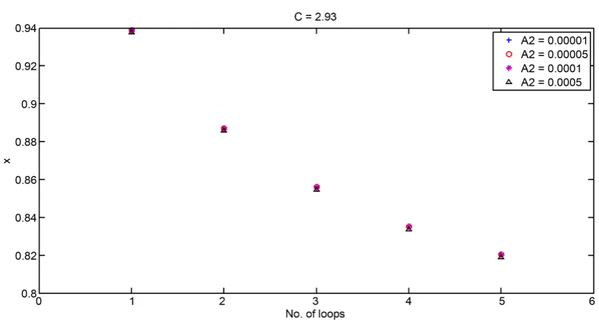
From Figure 8 and Figure 9, it can be observed that for given oblateness, location of periodic orbit moves away from second primary as number of loops in periodic orbit increase. Also, as oblateness increases, location of periodic orbit moves away from second primary.

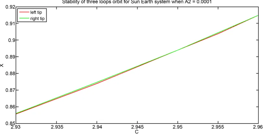
We have analyzed stability of periodic orbits from loop 1 to 5 for A2 = 0.00001,

0.00005, 0.0001 and 0.0005. Since stability behavior is similar for all these orbits, in this paper stability analysis for three loops orbit corresponding to A2 = 0.0001 is given.

Fig-ure 10 shows stability region for A2 = 0.0001 for three loop orbits. The left and right

Figure 4. Variation in location of single-loop periodic orbit around Sun-Mars system due to oblateness.

Figure 5. Variation in location of single-loop periodic orbit around Sun-Earth due to oblateness.

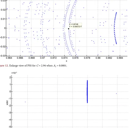
body required few amount of fuel than Hohmann transfer. Figure 11 shows amplitude for three loops orbit when A2 = 0.0001. It can be observe that there are two separatrices

at C = 2.95 and 2.96 where stability of the periodic orbit is zero as the size of the island is zero. For C = 2.94 we get maximum stability which is 0.0008. Figure 12 shows size of the island for C = 2.94 for three loops orbit when A2 = 0.0001 which is 0.0008 whereas

Figure 6. Variation in location of five loops periodic orbit around Sun-Mars system due to oblateness.

Figure 7. Variation in location of five loops periodic orbit around Sun-Earth system due to oblateness.

seen that size of this island is zero. Figure 14 shows three loops orbit corresponding to first separatrix when A2 = 0.0001. Figure 15 shows for C = 2.955 again size of island

in-creases and it becomes 0.0006, where as for C = 2.96 again size of island becomes zero, which is second separatrix as shown in Figure 16. Three loops orbit corresponding to second separatrix is given in Figure 17.

In Table 5 initial velocity of secondary body is denoted by V, D1 and D2 are the

dis-tance of secondary body from Mars and Sun respectively. V is in kms−1_{, D}

Figure 8. Variation in location of periodic orbit of secondary body around Sun and Mars for C = 2.93 due to num-ber of loops for different oblateness A2.

Figure 9. Variation in location of periodic orbit of secondary body around Sun-Earth system for C = 2.93 due to number of loops for different oblateness A2.

in km. Similar notations are used in Table 6 also. In Table 6 distance of secondary body from Earth is denoted by D1.

(

)

(

)

2 2

,

V = x + y+ +x

µ

V can be obtained using Equation (9).

Figure 10. Stability analysis for three loops orbit for Sun-Earth system when A2 = 0.0001.

Figure 11. Amplitude for three loops orbit for Sun-Earth system when A2 = 0.0001.

Distance D= ×L I (10) Velocity V = ×O J (11) where L is the distance between the centers of both primaries in km. O is the orbital velocity of second primary around first primary [2]. For Sun-Mars and Sun-Earth sys-tem L = 227,940,000 and 149,600,000 km respectively. Mean orbital velocity of Mars around Sun and Earth around Sun are 24.07 km∙sec−1 _{and 29.78 km∙sec}−1 _{respectively.}

Figure 12. Enlarge view of PSS for C = 2.94 when A2 = 0.0001.

Figure 13. Enlarge view of PSS of first separatrix for two loops orbit for C = 2.95 when A2 = 0.0001.

Figure 15. Enlarge view of PSS for C = 2.955 when A2 = 0.0001.

Figure 16. Enlarge view of PSS of second separatrix for three loops orbit for C = 2.96 when A2 = 0.0001.

2

2.96 0.94149 28.08 1.3336 2.1460 0.94136 28.08 1.3366 2.1457 0.94119 28.08 1.3405 2.1453 0.93985 28.11 1.3710 2.1422 2.95 0.92251 28.52 1.7662 2.1027 0.92239 28.53 1.7690 2.1024 0.92223 28.53 1.7726 2.1021 0.92096 28.55 1.8016 2.0992 2.94 0.9045 28.96 2.1768 2.0617 0.90438 28.96 2.1795 2.0614 0.90424 28.96 2.1827 2.0611 0.90302 28.99 2.2105 2.0583 2.93 0.88734 29.38 2.5679 2.0226 0.88722 29.39 2.5706 2.0223 0.88708 29.39 2.5738 2.0220 0.88592 29.41 2.6003 2.0193

3

2.96 0.91529 28.06 1.9308 2.0863 0.91514 28.06 1.9342 2.0859 0.91496 28.07 1.9383 2.0855 0.91348 28.10 1.9721 2.0821 2.95 0.89425 28.59 2.4104 2.0383 0.89412 28.59 2.4134 2.0380 0.89395 28.59 2.4172 2.0376 0.89258 28.62 2.4485 2.0345 2.94 0.87463 29.09 2.8576 1.9936 0.87449 29.09 2.8608 1.9933 0.87433 29.10 2.8645 1.9929 0.87305 29.12 2.8936 1.9900 2.93 0.85616 29.58 3.2786 1.9515 0.85604 29.58 3.2814 1.9512 0.85588 29.58 3.2850 1.9508 0.85467 29.61 3.3137 1.9480

4

2.96 0.89703 28.15 2.3470 2.0446 0.89688 28.15 2.3505 2.0443 0.89668 28.15 2.3550 2.0438 0.89515 21.18 2.3899 2.0404 2.95 0.8749 28.72 2.8515 1.9942 0.87476 28.72 2.8547 1.9939 0.87458 28.73 2.8588 1.9935 0.87316 28.76 2.8911 1.9902 2.94 0.85447 29.27 3.3172 1.9476 0.85433 29.27 3.3203 1.9473 0.85417 29.27 3.3240 1.9469 0.85284 29.30 3.3543 1.9439 2.93 0.8354 29.79 3.7518 1.9042 0.83528 29.79 3.7546 1.9039 0.83512 29.80 3.7582 1.9035 0.83388 29.82 3.7865 1.9007

5

2.96 0.88363 28.25 2.6525 2.0141 0.88347 28.25 2.6561 2.0137 0.88328 28.26 2.6605 2.0133 0.8817 28.29 2.6965 2.0097 2.95 0.8609 28.86 3.1706 1.9623 0.86075 28.86 3.1740 1.9619 0.86057 28.86 3.1781 1.9615 0.85912 28.89 3.2112 1.9582 2.94 0.84004 29.43 3.6461 1.9147 0.83991 29.43 3.6490 1.9144 0.83974 29.43 3.6529 1.9141 0.83839 29.46 3.6837 1.9110 2.93 0.82068 29.98 4.0874 1.8706 0.82056 29.98 4.0901 1.8703 0.8204 29.98 4.0937 1.8700 0.81914 30.01 4.1225 1.8671

Table 6. Location, velocity and distance of orbit from both primaries for A2 = 0.00001, 0.00005, 0.0001, 0.0005 for Sun-Earth system.

No. of loop C A2 = 0.00001 A2 = 0.00005 A2 = 0.0001 A2 = 0.0005

x _(km∙secV −1_{) (10}D7 _km) 1 ₍₁₀D8 _{km) x} 2 _(km∙secV −1_{) (10}D7 _km) 1 ₍₁₀D8 _{km) x} 2 _(km∙secV −1_{) (10}D7 _km) 1 ₍₁₀D8 _{km) x} 2 _(km∙secV −1_{) (10}D7 _km) 1 ₍₁₀D8 _km) 2

1

2.96 0.983 35.32 0.2542 1.4705 0.9829 35.32 0.2557 1.4704 0.9828 35.33 0.2572 1.4702 0.9817 35.36 0.2737 1.4686 2.95 0.9679 35.70 0.4801 1.4479 0.96782 35.70 0.4813 1.4478 0.9677 35.70 0.4831 1.4476 0.9666 35.72 0.4996 1.4460 2.94 0.95325 36.09 0.6993 1.4260 0.95315 36.09 0.7008 1.4259 0.95304 36.09 0.7024 1.4257 0.952 36.11 0.7180 1.4241 2.93 0.939 36.47 0.9125 1.4047 0.9389 36.47 0.9140 1.4045 0.93877 36.48 0.9159 1.4044 0.93775 36.50 0.9312 1.4028

2

2.96 0.94155 34.75 0.8743 1.40856 0.9414 34.75 0.8766 1.4083 0.94125 34.75 0.8788 1.4081 0.9399 34.78 0.8990 1.4060 2.95 0.92255 35.30 1.1586 1.3801 0.92244 35.30 1.1602 1.3799 0.92226 35.30 1.1629 1.3797 0.921 35.33 1.1817 1.3778 2.94 0.90455 35.83 1.4278 1.3532 0.90442 35.84 1.4298 1.3530 0.90426 35.84 1.4322 1.3527 0.90305 35.87 1.4503 1.3509 2.93 0.88737 36.36 1.6848 1.3275 0.88725 36.36 1.6866 1.3273 0.8871 36.36 1.6889 1.3271 0.88595 36.39 1.7061 1.3253

3

2.96 0.91535 34.72 1.2663 1.3693 0.9152 34.73 1.2685 1.3691 0.915 34.73 1.2715 1.3688 0.91354 34.77 1.2933 1.3666 2.95 0.8943 35.37 1.5812 1.3378 0.89416 35.37 1.5833 1.3376 0.894 35.38 1.5857 1.3374 0.89262 35.41 1.6063 1.3353 2.94 0.87465 35.99 1.8751 1.3084 0.87453 36.00 1.8769 1.3083 0.87438 36.00 1.8792 1.3080 0.87309 36.03 1.8985 1.3061 2.93 0.8562 36.60 2.1512 1.2808 0.85608 36.60 2.1529 1.2807 0.85592 36.60 2.1553 1.2804 0.8547 36.63 2.1736 1.2786

4

2.96 0.8971 34.83 1.5393 1.34206 0.89695 34.83 1.5415 1.3418 0.89675 34.83 1.5445 1.3415 0.8952 34.87 1.5677 1.3392 2.95 0.87495 35.54 1.8707 1.3089 0.87482 35.54 1.8726 1.3087 0.87464 35.54 1.8753 1.3084 0.87321 35.58 1.8967 1.3063 2.94 0.8545 36.21 2.1766 1.2783 0.85438 36.21 2.1784 1.2781 0.85421 36.22 2.1809 1.2779 0.85289 36.25 2.2007 1.2759 2.93 0.83544 36.86 2.4617 1.2498 0.83532 36.86 2.4635 1.2496 0.83516 36.87 2.4659 1.2494 0.83392 36.90 2.4845 1.2475

5

number of loop as A2 increases initial velocity increases and D1 increases so, D2

de-creases. So, the effect of Jacobi constant C and oblateness A2 is opposite in nature. For

given value of A2 and C as number of loops increases, D1 increases and D2 decreases

where as V decreases up to loops 1 - 3 and then increases from 3 - 5-loop orbits. From

Table 5, it is observed that single-loop orbit for A2 = 0.00001 is closest to Mars and this

distance is 3.886 × 107 _{km. which is obtained using C = 2.96. Similar notations are used}

in Table 6 also.

From Table 6, it is observed that single-loop orbit for A2 = 0.00001 is closest to Earth

and this distance is 2.542 × 107 _{km. which is obtained using C = 2.96. Here D} 1 is the

distance of secondary body from Earth.

4. Prediction of Orbit through Regression Analysis

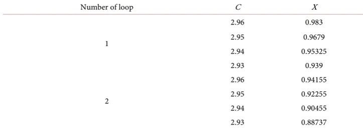
The locations of single-loop and two loops periodic orbits obtained for different values of C for Sun-Mars system A2 = 0.00001 from PSS is displayed in Table 7. Using

regres-sion analysis we have displayed the predicted position of the orbit for different values of

C. The predicted and exact values of positions together with error estimates are dis-played in Table 8. The best fit curve for single-loop is a straight line with equation

Table 7. Variation in location of periodic orbit when A2 = 0.00001 for Sun-Mars system.

Number of loop C X

1

2.96 0.98295 2.95 0.9679 2.94 0.95324 2.93 0.93896

2

2.96 0.94149 2.95 0.92251 2.94 0.9045 2.93 0.88734

Table 8. Prediction and error for periodic orbit when A2 = 0.00001 for Sun-Mars system. Number of loop C Predicted Exact Error

1

2.92 0.92372 0.92508 0.00136 2.925 0.93105 0.93198 0.00093 2.935 0.94571 0.94605 0.00034 2.945 0.96037 0.9605 0.00013 2.955 0.97503 0.9754 0.00037 2.965 0.98969 0.99069 0.001

2

It can be observed that as C increases the error between the predicted and exact val-ues of the position of periodic orbits increases. The PSS together with regression analy-sis will help one to locate the position of the periodic orbit with less effort, using the predicted positions from the analysis.

The variation of position x with oblateness A2 for Sun-Mars system for fixed value of

C = 2.96 using PSS is shown in Table 11. The predicted and exact values of the position of orbits together with error estimates using regression analysis are shown in Table 12. For single-loop the best fit regression curve is 2

2 2

500.7 2.5 0.983

x= − ×A − ×A + with

R2 _{= 1, where as for two loops orbit} 2

2 2

39.14 3.329 0.941

x= − ×A − ×A + with R2 = 1. Table 9. Variation in location of periodic orbit when A2 = 0.0005 for Sun-Mars system.

Number of loop C X

1

2.96 0.9816 2.95 0.9666 2.94 0.95196 2.93 0.93772

2

2.96 0.93985 2.95 0.92096 2.94 0.90302 2.93 0.88592

Table 10. Prediction and error for periodic orbit when A2 = 0.0005 for Sun-Mars system.

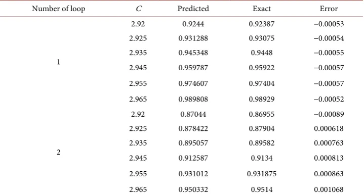
Number of loop C Predicted Exact Error

1

2.92 0.9244 0.92387 −0.00053 2.925 0.931288 0.93075 −0.00054 2.935 0.945348 0.9448 −0.00055 2.945 0.959787 0.95922 −0.00057 2.955 0.974607 0.97404 −0.00057 2.965 0.989808 0.98929 −0.00052

2

The variation of position x for different values of C for one-loop and two loops orbit for A2 = 0.00001 for Sun-Earth system is shown in Table 13.

Using regression analysis we have displayed predicted and exact values of position together with error estimates are shown in Table 14. As in the case of Sun-Mars system the error estimates decreases, with increase in C for both single-loop and two-loops or-bits. The best fit curve for single-loop orbit is given by x=1.466× −C 3.358 with R2 =

0.999, and for two loops orbit regression line x=1.805× −C 4.402 with R2 = 0.999.

Similar estimates are displayed for A2 = 0.00005 in Table 15 and Table 16, for Sun-

Earth system.

For single-loop orbit regression curve is given by 2

2.125 11.05 15.07

x= ×C − × +C

Table 11. Variation in location of periodic orbit when C = 2.96 for Sun-Mars system.

Number of loop A2 X

1

0.00001 0.98295 0.00005 0.98285 0.0001 0.98272 0.0005 0.9816

2

0.00001 0.94149 0.00005 0.94136 0.0001 0.94119 0.0005 0.93985

Table 12. Prediction and error for periodic orbit when C = 2.96 for Sun-Mars system.

Number of loop A2 Predicted Exact Error

1

0.000025 0.982937187 0.98293 −7.187E−06 0.000075 0.982809684 0.9828 −9.683E−06 0.00025 0.982343706 0.98233 −1.3706E−05 0.00075 0.980843356 0.98095 0.000106644

2

0.000025 0.940916751 0.94145 0.000533249 0.000075 0.940750105 0.94128 0.000529895 0.00025 0.940165304 0.94069 0.000524696 0.00075 0.938481234 0.93902 0.000538766

Table 13. Variation in location of periodic orbit when A2 = 0.00001 for Sun-Earth system.

Number of loop C X

1

2.96 0.983 2.95 0.9679 2.94 0.95325 2.93 0.939

2

2.965 0.98869 0.99072 0.00203

2

2.92 0.8686 0.87095 0.00235 2.925 0.877625 0.87909 0.001465 2.935 0.895675 0.89588 0.000205 2.945 0.913725 0.91342 −0.0003 2.955 0.931775 0.9319 0.000125 2.965 0.949825 0.95147 0.001645

Table 15. Variation in location of periodic orbit when A2 = 0.00005 for Sun-Earth system.

Number of loop C X

1

2.96 0.9817 2.95 0.9666 2.94 0.952 2.93 0.93775

2

2.96 0.9414 2.95 0.92244 2.94 0.90442 2.93 0.88725

Table 16. Prediction and error for periodic orbit when A2 = 0.00005 for Sun-Earth system.

Number of loop C Predicted Exact Error

1

2.92 0.9226 0.92501 0.00241 2.925 0.929453 0.93189 0.002437 2.935 0.943478 0.94599 0.002512 2.945 0.957928 0.96044 0.002512 2.955 0.972803 0.97532 0.002517 2.965 0.988103 0.99062 0.002517

2

2.92 0.87964 0.87083 −0.00881 2.925 0.887672 0.87896 −0.00871 2.935 0.904407 0.89573 −0.00868 2.945 0.922037 0.91333 −0.00871 2.955 0.940562 0.9318 −0.00876 2.965 0.959982 0.9513 −0.00868

with R2 _{= 1 and for two-loops orbit regression curve is given by}

2

4.475 24.55 34.41

The variation of position x with oblateness A2 for Sun-Earth system is shown in

Ta-ble 17 for a fix value of C = 2.96.

The predicted and exact value of position together with error estimates are shown in

Table 18.

The equation of the best fit curve for single-loop is 2

2 2

1056 2.105 0.983

x= − ×A − ×A + with R2 = 1, where as for two-loops orbit regres-sion curve is 2

2 2

58.59 3.325 0.941

x= − ×A − ×A + with R2 = 1.

5. Conclusions

In this paper, we have studied the effect of oblateness on the position, shape and size of closed periodic orbit with loops varying from 1 to 5 for Sun-Mars and Sun-Earth sys-tems, respectively. It is concluded that for given number of loops and given C, as ob-lateness increases, location of periodic orbit moves towards Sun. For given C and given oblateness, as number of loops increases, location of periodic orbits shifts towards Sun. Also, for given value of oblateness and given number of loops, as C decreases, location of periodic orbit moves towards Sun. Also, period of the orbit increases as number of loops increases. It is also observed that single-loop orbit is closest to second primary body. Further, as number of loops decreases, width of the orbit increases. The distance of closest approach of the infinitesimal particle from the smaller primary increases with oblateness and number of loops for a given C. Thus, the present analysis of the two sys-tems—Sun-Mars and Sun-Earth systems—using PSS technique reveals that A2 and C has

Table 17. Variation in location of periodic orbit when C = 2.96 for Sun-Earth system.

Number of loop A2 X

1

0.00001 0.983 0.00005 0.9829

0.0001 0.9828 0.0005 0.9817

2

0.00001 0.94155 0.00005 0.9414

0.0001 0.94125 0.0005 0.9399

Table 18. Prediction and error for periodic orbit when C = 2.96 for Sun-Earth system.

Number of loop A2 Predicted Exact Error

1

0.000025 0.982946715 0.98294 −6.715E−06 0.000075 0.982836185 0.98283 −6.185E−06 0.00025 0.98240775 0.9824 −7.75E−06 0.00075 0.98082725 0.981 0.00017275

2

creases, initial velocity increases and distance of spacecraft from second primary in-creases. So, distance of spacecraft from first primary dein-creases. Thus, the effect of Jaco-bi constant C and oblateness coefficient A2 is opposite in nature. For given value of

oblateness coefficient and Jacobi constant, as number of loops increases, distance of spacecraft from second primary increases and distance of spacecraft from first primary decreases where as initial velocity of spacecraft decreases up to loops 1 - 3 and then in-creases from 3 - 5. It is further observed that for Sun-Mars system, single-loop orbit for

A2 = 0.00001 and C = 2.96 is closest to Mars and this distance is 3.886 × 107 km.

Whe-reas for Sun-Earth system, single-loop orbit for A2 = 0.00001 and C = 2.96 is closest to

Earth and this distance is 2.542 × 107 _{km. Since stability of this class of periodic orbits is}

very low, it can be used for designing low-energy trajectory design for space mission.

Acknowledgements

The authors thank Mrs. Pooja Dutt, Applied Mathematics Division, Vikram Sarabhai Space Centre (ISRO), Thiruvananthapuram, India for her constructive comments.

References

[1] Koon, W.S., Lo, M.W., Marsden, J.E. and Ross, S. (2001) Low Energy Transfer to the Moon. Celestial Mechanics and Dynamical Astronomy. Celestial Mechanics and Dynamical As-tronomy, 81, 63-73. https://doi.org/10.1023/A:1013359120468

[2] Koon, W.S., Lo, M.W., Marsden, J.E. and Ross, S. (2011) Dynamical Systems, the Three- Body Problem and Space Mission Design.

http://www.cds.caltech.edu/~marsden/books/Mission_Design.html

[3] Szebehely, V. (1967) Theory of Orbits. Academic Press, San Diego.

[4] Murray, C.D. and Dermot, S.F. (1999) Solar System Dynamics. Cambridge University Press, Cambridge.

[5] Dutt, P. and Sharma, R.K. (2010) Analysis of Periodic and Quasi-Periodic Orbits in the Earth-Moon System. Journal of Guidance, Control, and Dynamics, 33,1010-1017.

https://doi.org/10.2514/1.46400

[6] Dutt, P. and Sharma, R.K. (2011) Evolution of Periodic Orbits in the Sun-Mars System.

Journal of Guidance, Control, and Dynamics, 34,635-644. https://doi.org/10.2514/1.51101

[7] Safiyabeevi, A. and Sharma, R.K. (2011) Oblateness Effect of Saturn on Periodic Orbits in the Saturn-Titan Restricted Three-Body Problem. Astrophysics and Space Science, 340, 245-261.https://doi.org/10.1007/s10509-012-1052-3

[8] Dutt, P. and Sharma, R.K. (2012) On the Evolution of the “f” Family in the Restricted Three-Body Problem. Astrophysics and Space Science, 340,63-70.

[9] Tsirogiannis, G.A. and Douskos, C.N. and Perdios, E.A. (2006)Computation of the Liapu-nov Orbits in the Photogravitational RTBP with Oblateness. Astrophysics and Space Science, 305,389-398. https://doi.org/10.1007/s10509-006-9171-3

[10] Perdiou, A.E., Perdios, E.A. and Kalantonis, V.S. (2012)Periodic Orbits of the Hill Problem with Radiation and Oblateness. Astrophysics and Space Science, 342,19-30.

https://doi.org/10.1007/s10509-012-1145-z

[11] Elshaboury, S.M., Abouelmagd, E.I., Kalantonis, V.S. and Perdios, E.A. (2016) The Planar Restricted Three-Body Problem When Both Primaries Are Triaxial Rigid Bodies: Equili-brium Points and Periodic Orbits. Astrophysics and Space Science, 361, 315.

https://doi.org/10.1007/s10509-016-2894-x

[12] Mittal, A., Ahmad, I. and Bhatnagar, K.B. (2009)Periodic Orbits Generated by Lagrangian Solutions of the Restricted Three Body Problem When One of the Primaries Is an Oblate Body. Astrophysics and Space Science, 319, 63-73.

https://doi.org/10.1007/s10509-008-9942-0

[13] Mittal, A., Ahmad, I. and Bhatnagar, K.B. (2009) Periodic Orbits in the Photogravitational Restricted Problem with the Smaller Primary an Oblate Body. Astrophysics and Space Science, 323,65-73. https://doi.org/10.1007/s10509-009-0038-2

[14] Perdios, E.A. and Kalantonis, V.S. (2006)Computation of the Liapunov Orbits in the Pho-togravitational RTBP with Oblateness. Astrophysics and Space Science, 305, 389-398.

https://doi.org/10.1007/s10509-006-9171-3

[15] Broucke, R.A. (1968) Technical Report. Vol. 32, Jet Propulsion Lab., Pasadena.

[16] Jefferys, W.H. (1971) An Atlas of Surfaces of Section for the Restricted Problem of Three Bodies. Published at the Department of Astronomy of the University of Texas at Austin, Ser. II, 3, 6.

[17] Smith, R.H. (1991) The Onset of Chaotic Motion in the Restricted Problem of Three Bo-dies. PhD Thesis, University of Texas at Austin, Austin.

[18] Contopoulos, G. (1991) Periodic Orbits and Chaos around Two Fixed Black Holes. Pro-ceedings of the Royal Society of London, 435, 551-562.

[19] Poincare, H. (1892) Celeste. Vol. 1, Gauthier-Villas, Paris, 82.

[20] Winter, O.C. and Murray, C.D. (1994) QMW Notes No. 16. Queen Marry and Westfield College, London.

[21] Winter, O.C. and Murray, C.D. (1994) QMW Notes No. 17. Queen Marry and Westfield College, London.

[22] Winter, O.C. and Murray, C.D. (1997)Resonance and Chaos. Astronomy & Astrophysics, 319,290-304.

[23] Winter, O.C. and Murray, C.D. (1997)Resonance and Chaos. II. Exterior Resonances and Asymmetric Libration. Astronomy & Astrophysics, 328,399-408.

[24] Pathak, N., Sharma, R.K. and Thomas, V.O. (2016) Evolution of Periodic Orbits in the Sun-Saturn System. International Journal of Astronomy and Astrophysics, 6,175-197.

https://doi.org/10.4236/ijaa.2016.62015

[25] Pathak. N. and Thomas, V.O. (2016) Evolution of the “f” Family Orbits in the Photo Gravi-tational Sun-Saturn System with Oblateness. International Journal of Astronomy and As-trophysics, 9, 254-271.

Submit or recommend next manuscript to SCIRP and we will provide best service for you:

Accepting pre-submission inquiries through Email, Facebook, LinkedIn, Twitter, etc. A wide selection of journals (inclusive of 9 subjects, more than 200 journals)

Providing 24-hour high-quality service User-friendly online submission system Fair and swift peer-review system

Efficient typesetting and proofreading procedure

Display of the result of downloads and visits, as well as the number of cited articles Maximum dissemination of your research work