A Remark on the Topology at Infinity of a Polynomial Mapping F: Cn→Cn via Intersection Homology

http://www.scirp.org/journal/apm ISSN Online: 2160-0384 ISSN Print: 2160-0368

A Remark on the Topology at Infinity of a

Polynomial Mapping

n

n

F :



→



via

Intersection Homology

Nguyen Thi Bich Thuy

UNESP, Universidade Estadual Paulista, “Júlio de Mesquita Filho”, São José do Rio Preto, Brazil

Abstract

In [1], Guillaume and Anna Valette associate singular varieties VF to a polynomial

mapping _F:_n_→n. In the case _F:2_→2, if the set

( )

0

K F of critical

values of F is empty, then F is not proper if and only if the 2-dimensional

homology or intersection homology (with any perversity) of VF is not trivial. In [2],

the results of [1] are generalized in the case F:n→n where n≥3, with an additional condition. In this paper, we prove that for a class of non-proper generic dominant polynomial mappings, the results in [1] and [2] hold also for the case that the set K0

( )

F is not empty.

Keywords

Polynomial Mappings, Intersection Homology, Singularities

1. Introduction

In [1], Guillaume and Anna Valette provide a criteria for properness of a polynomial mapping 2 2

:

F  → . They construct a real algebraic singular variety V_F satisfying

the following property: if the set of critical values of F is empty then F is not

proper if and only if the 2-dimensional homology or intersection homology (with any perversity) of VF is not trivial ([1], Theorem 3.2). This result provides a new approach

for the study of the well-known Jacobian Conjecture, which is still open until today, even in the two-dimensional case (see, for example, [3]). In [2], the result of [1] is generalized in the general case _F:_n→_n, where

3

n≥ , with an additional

condition ([2], Theorem 4.5). The variety VF is a real algebraic singular variety of

dimension 2n in some 2n q+ , where q>0, the singular set of which is contained in

How to cite this paper: Thuy, N.T.B. (2016) A Remark on the Topology at Infinity of a Polynomial Mapping : n n

F  → via In-

tersection Homology. Advances in Pure Mathematics, 6, 1037-1052.

http://dx.doi.org/10.4236/apm.2016.613076

Received: November 8, 2016 Accepted: December 25, 2016 Published: December 28, 2016

Copyright © 2016 by author and Scientific Research Publishing Inc. This work is licensed under the Creative Commons Attribution International License (CC BY 4.0).

( )

(

0

)

{ }

0

q F

K F ∪S × _ , where K0

( )

F is the set of critical values and SF is the

asymptotic set of F.

This paper proves that if 2 2

:

F  → is a non-proper generic dominant poly-

nomial mapping, then the 2-dimensional homology and intersection homology (with any perversity) of VF are not trivial. We prove that this result is also true for a

non-proper generic dominant polynomial mapping F:n→n

(

n≥3

)

, with the

same additional condition than in [2]. To prove these results, we use the Transversality Theorem of Thom: if F is non-proper generic dominant polynomial mapping, we

can construct an adapted

(

2,p

)

-allowable chain (in generic position) providing non

triviality of homology and intersection homology of the variety VF, for any perversity p (Theorems 5.1 and 5.2).

In order to compute the intersection homology of the variety VF in the case

( )

0

K F ≠ ∅, we have to stratify the set K0

( )

F ∪SF. Furthermore, the intersection

homology of the variety VF does not depend on the stratification if we use a locally

topologically trivial stratification. It is well-known that a Whitney stratification is a Thom-Mather stratification and a Thom-Mather stratification is a locally topologically trivial stratification (see [4][5][6][7]). In order to prove the main result, we use two facts: In [6], Thom defined a partition of the set K0

( )

F by “constant rank”, which is a local Thom-Mather stratification; in [2], the authors provide a Whitney stratification of the asymptotic set SF. One important point for the proof of the princial results of this

paper is the following: we show that in general the set K0

( )

F is not closed, so we cannot define a (global) stratification of K0

( )

F satisfying the frontier condition. Hence, we cannot define a (global) Thom-Mather stratification of K0

( )

F . However, we prove that the set K0

( )

F ∪SF is closed and K0

( )

F ∪SF=K0

( )

F ∪SF. This fact

allows us to show that there exists a Thom-Mather stratification of the set K0

( )

F ∪SF

compatible with the partition of the set K0

( )

F defined by Thom in [6] and com- patible with the Whitney stratification of the set SF defined in [2] (Theorem 4.6).

This paper provides also some examples to light the results. Moreover, these ex- amples provide also some topological properties of the well-known critical values set

( )

0

K F associated to a complex polynomial mapping F:n→n, for instance: in general, the set K0

( )

F is not closed; the set K0

( )

F ∪SF is not smooth; K0

( )

F ∪SF

is not pure dimensional if F is not dominant. Via these examples, we make clear also

the well-known Thom-Mather partition of K0

( )

F defined by Thom in [6].

2. Preliminaries

In this section we set-up our framework. All the varieties we consider in this article are semi-algebraic.

2.1. Intersection Homology

We briefly recall the definition of intersection homology. For details, we refer to the fundamental work of M. Goresky and R. MacPherson [8] (see also [4]).

stratification of V is the data of a finite semi-algebraic filtration

1 0 1 ,

m m

V =V ⊃V ₋ ⊃⊃V ⊃V₋ = ∅

such that for every i, the set V V_i\ _i−1 is either an emptyset or a manifold of dimension

i. A connected component of V Vi\ i−1 is called a stratum of V.

Let Si be a stratum of V and Si its closure in V. If Si\Si is the union of strata

of V, for all strata Si of V , then we say that the stratification of V satisfies the

frontier condition.

Definition 2.2 (see [6][9]). Let V be a variety in a smooth variety M . We say that

a stratification of V is a Thom-Mather stratification if each stratum S_i is a dif-

ferentiable variety of class _∞ _{and if for each} i

S, we have:

)

a an open neighbourhood (tubular neighbourhood) T_i of S_i in M ,

)

b a continuous retraction πi of Ti on Si,

)

c a continuous function ρi:Ti→

[ [

0,∞ which is

∞

 on the smooth part of

i V∩T,

such that S_i=

{

x∈T_i:ρ

( )

x =0

}

and if Si⊂Sj, then

i) the restricted mapping

(

π ρi, i

)

:Ti∩Sj → ×Si

[ [

0,∞ is a smooth immersion,

ii) for x∈ ∩Ti Tj such that πj

( )

x ∈Ti, we have the following relations of com-

mutation:

1) π πi j

( )

x =πi

( )

x ,

2) ρ πi j

( )

x =ρi

( )

x ,

when the two members of these formulas are defined.

A Thom-Mather stratification satisfies the frontier conditions.

We denote by cL the open cone on the space L, the cone on the empty set being a

point. Observe that if L is a stratified set then cL is stratified by the cones over the

strata of L and an additional 0-dimensional stratum (the vertex of the cone). Definition 2.3. A stratification of V is said to be locally topologically trivial if for

every x∈V Vi \ i−1, i≥0, there is an open neighborhood Ux of x in V , a stratified

set L and a semi-algebraic homeomorphism

( )

: x 0;1i ,

h U → ×cL

such that h maps the strata of U_x (induced stratification) onto the strata of

( )

0;1i×cL (product stratification).

Theorem 2.4 (see [6] [7]). A Thom-Mather stratification is a locally topologically trivial stratification.

Definition 2.5 ([7]). One says that the Whitney

( )

b condition is realized for a

stratification if for each pair of strata

(

S S, ′

)

and for any y∈S one has: Let

{ }

xn

be a sequence of points in S′ with limit y and let

{ }

yn be a sequence of points in S tending to y, assume that the sequence of tangent spaces

{ }

T Sx_n ′ admits a limit

T for n tending to +∞ (in a suitable Grassmanian manifold) and that the sequence

of directions x yn n admits a limit λ for n tending to +∞ (in the corresponding

projective manifold), then λ∈T.

tification.

Theorem 2.6 ([5]). Every Whitney stratification is a Thom-Mather stratification, hence satisfies the topological triviality.

The definition of perversities has originally been given by Goresky and MacPherson: Definition 2.7. A perversity is an (m + 1)-uple of integers p=

(

p p p p0, 1, 2, 3,,pm

)

such that p0 = p1=p2 =0 and pα+1∈

{

pα,pα+1

}

, for α≥2.

Traditionally we denote the zero perversity by 0=

(

0, 0,, 0

)

, the maximal per-

versity by t =

(

0, 0, 0,1,,m−2

)

, and the middle perversities by

2 0, 0, 0, 0,1,1, ,

2

m m=  _ − __

 

   (lower middle) and

1 0, 0, 0,1,1, 2, 2, ,

2

m

n=  _ − _

 

  

(upper middle). We say that the perversities p and q are complementary if p+ =q t .

Let V be a semi-algebraic variety such that V admits a locally topologically trivial

stratification. We say that a semi-algebraic subset Y ⊂V is

( )

p i, -allowable if

(2.8) dim

(

Y∩V_m−α

)

≤ − +i α p_α for all α≥2. Define p

( )

i

IC V to be the -vector subspace of C Vi

( )

consisting in the chains

ξ such that ξ is

( )

p i, -allowable and ∂ξ is

(

p i, −1

)

-allowable.

Definition 2.9 The _ith intersection homology group with perversity

p, with real

coefficients, denoted by p

( )

i

IH V , is the _ith homology group of the chain complex

( )

*

p

IC V .

Notice that, the notation ,

( )

*

p c

IH V refers to the intersection homology with

compact supports, the notation ,

( )

*

p cl

IH V refers to the intersection homology with

closed supports. In the compact case, they coincide.

Theorem 2.10 ([8][10]) The intersection homology is independent on the choice of the stratification satisfying the locally topologically trivial conditions.

The Poincaré duality holds for the intersection homology of a (singular) variety: Theorem 2.11 (Goresky, MacPherson [8]). For any orientable compact stratified semi-algebraic m-dimensional variety V , the generalized Poincaré duality holds:

( )

( )

,

p q

k m k

IH V IH − V

where p and q are complementary perversities.

For the non-compact case, we have:

( )

( )

, ,

.

p c q cl

k m k

IH V IH − V

2.2. The Asymptotic Set

Let _F:_n_→n be a polynomial mapping. Let us denote by F

S the set of points at

which F is non proper, i.e.,

(2.12) _F:

{

n such that

{ }

_k n, _k tends to infinity and

( )

_k tends to

}

k

S = a∈ ∃ x _∈⊂ x F x a

where xk is the Euclidean norm of xk in n

 . The set SF is called the asymptotic

In this paper, we will use the following important theorem:

Theorem 2.13. [11] Let F:n→n be a polynomial mapping. If F is do-

minant, i.e.,

( )

n n

F  = , then S_F is either an empty set or a hypersurface.

3. The Variety

V

F

We recall in this section the construction of the variety VF and the results obtained in [1] and [2]: Let _F:_n→_n be a polynomial mapping. We consider

F as a real

mapping 2 2

: n n

F  → . By Sing F we mean the set of critical points of F. Thanks

to the lemma 2.1 of [1], there exists a covering

{

U1,,Up

}

of

( )

2

\ Sing

n F

M = F

by semi-algebraic open subsets (in 2n) such that on every element of this covering,

the mapping F induces a diffeomorphism onto its image. We may find some semi-

algebraic closed subsets Vi ⊂Ui (in MF) which cover MF as well. By the Mosto-

wski’s Separation Lemma (see [12], p. 246), for each i=1,,p, there exists a Nash

function ψ_i:M_F→, such that ψ_i is positive on V_i and negative on M_F \U_i. We

can choose the Nash functions ψi such that ψi

( )

xk tends to zero where

{ }

xk is a

sequence in MF tending to infinity. We define

(

1

)

( )

: , , , ,

F p F

V = Fψ ψ M

that means, VF is the closure of the image of MF by

(

F,ψ1,,ψp

)

.

The variety VF is a real algebraic singular variety of dimension 2n in

2n q+  , with 0

q> , the singular set of which is contained in

(

0

( )

)

{ }

0

q F

K F ∪S × _ , where K0

( )

F is the set of critical values and SF is the asymptotic set of F.

Theorem 3.1 ([2]). Let F:n→n be a generically finite polynomial mapping with nowhere vanishing Jacobian. There exists a filtration of VF:

2 2 1 2 2 1 0 1

F n n n

V =V ⊃V ₋ ⊃V ₋ ⊃⊃V ⊃V ⊃V₋ = ∅

such that:

1) for any i<n, V_{2 1i+} =V_2i,

2) the corresponding stratification satisfies the Whitney

( )

b condition.

Recall the condition “F is nowhere vanishing Jacobian” means that the set of critical

values K0

( )

F of F is an emptyset.

The following corollary comes directly from the Theorem 3.1 above.

Corollary 3.2. Let _F:_n_→n be a generically finite polynomial mapping. Then

there exists a Whitney stratification of the asymptotic set SF.

Theorem 3.3 ([1]). Let _F:2_→2 be a polynomial mapping with nowhere

vanishing Jacobian. The following conditions are equivalent: 1) F is non proper,

2) H V2

( )

F ≠0,

3) 2

( )

0

p F

IH V ≠ for any perversity p,

4) 2

( )

0

p F

IH V ≠ for some perversity p.

Form here, we denote by ˆ

i

F the homogeneous component of Fi of highest degree,

or the leading form of Fi.

Jacobian. If _Rank

( )

ˆ _{1, , 1}

i i n

DF n

= ≥ −

 _ , where Fˆi is the leading form of Fi, then the

following conditions are equivalent: 1) F is non proper,

2) H V2

( )

F ≠0,

3) 2

( )

0

p F

IH V ≠ for any (or some) perversity p

4) 2 2

( )

0

p n F

IH − V ≠ , for any (or some) perversity p.

Notice that with the notations H V*

( )

(resp. *

( )

p

IH V ), we mean the homology

(resp., the intersection homology) with both compact supports and closed supports. Remark 3.5. There exist may-be a lots of varieites VF associated to the same

polynomial mapping F:n→n, but for any variety V_F, its properties in the

Theorems 3.3 and 3.4 do not change.

The purpose of this paper is to prove that if F:n →n

(

n≥2

)

is a non-proper

generic dominant polynomial mapping, then the 2-dimensional homology and in- tersection homology (with any perversity) of VF are not trivial. In order to compute

the intersection homology of the variety VF in the case K0

( )

F ≠ ∅, we have to stratify the set K0

( )

F ∪SF. Furthermore, the intersection homology of the variety VF

does not depend on the stratification of VF if we use a locally topologically trivial

stratification. By theorem 2.4, a Thom-Mather stratification is a locally topologically trivial stratification. In the following section, we provide an explicit Thom-Mather stratification of the set K0

( )

F ∪SF.

4. A Thom-Mather Stratification of the Set

K

₀

( )

F

∪

S

_F

We begin this section by giving an example to show that in general the set K0

( )

F of a polynomial mapping F:n→n is neither closed, nor smooth, nor pure dimen- sional. Recall that a set X is pure dimensional of dimension m if any point of this

set admits a m-dimensional neighbourhood in X.

Example 4.1. Let us consider the polynomial mapping (1 2 3) ( 1 2 3)

3 3

, , , ,

: _{x x x}

F  →_{α α α}

such that

(

)

(

3

)

1, 2, 3 1 1 2 3, 2 3, 3 1 .

F x x x = x −x x x x x x x

Then, the jacobian determinant JF

( )

x of F is given by

(

)

2 1 3 31 2 3

x x x −x x . If

( )

0

F

J x = then x₁=0 or x₃=0 or 3x12=x x2 3. So we have the following cases: + if x1=0 then F

(

0,x x2, 3

) (

= 0,x x2 3, 0

)

and the axis 0α2 is contained in

( )

0

K F ,

+ if x3=0 then

(

)

(

)

3 1, 2, 0 1, 0, 0

F x x = x and the axis 0α1 is contained in K0

( )

F , + if 2

1 2 3

3x =x x then

(

)

(

3 2

)

(

)

1, 2, 3 2 1, 3 1, 3 1 1, 2, 3

F x x x = − x x x x = α α α . We observe that:

if x1=0 then α1=α2=α3=0; If x1≠0 then α1≠0 and α2 ≠0. Moreover,

since 2 1 2 3

3x =x x and x₁≠0, then x₃≠0, this implies α₃≠0. Furthermore, we

have 2 3

1 2

27α =4α . Let

( )

{

(

)

(1 2 3)

}

3 2 3

1, 2, 3 α α α, , : 27 1 4 2, 1 0, 2 0, 3 0 ,

α α α α α α α α

= ∈ = ≠ ≠ ≠

S

So, we have K0

( ) ( )

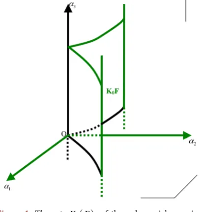
F = S ∪0α1∪0α2 (see Figure 1).

Notice that K0

( )

F does not contain neither 0α3\ 0

{ }

, nor the curve

( )

C of equation 2 3

1 2

27α =4α in the plane

(

0α α_{1 2}

)

. However

{ }

0 ⊆K₀

( )

F and this is the

singular point of K0

( )

F . So, the set K0

( )

F is neither closed, nor smooth, nor pure dimensional.

From the example 4.1, in general the set K0

( )

F is not closed, so we cannot stratify

( )

0

K F in such a way that the stratification satisfies the frontier condition. The

following proposition allows us to provide a stratification satisfying the frontier con- dition of the set K0

( )

F ∪SF.

Proposition 4.2. The set K0

( )

F ∪SF is closed. Moreover, we have

( )

( )

0 F 0 F.

K F ∪S =K F ∪S

To prove this proposition, we need the three following lemmas.

Lemma 4.3. For a polynomial mapping F:n→n, the set of the solutions of

( )

0

F

J x = is closed, where JF

( )

x is the jacobian determinant of F at x.

Chứng minh. Considering a sequence

{ }

xk contained in the set

( )

{

x∈n: JF x =0

}

such that xk tends to x0. Since F is a polynomial mapping,

then JF

( )

x is also a polynomial mapping and JF

( )

x is continuous. Hence

( )

F k

J x tends to JF

( )

x0 . Since JF

( )

xk =0 for all xk, we have JF

( )

x0 =0. So 0

x belongs to the set

{

x J: F

( )

x =0

}

. We conclude that the set of the solutions of

( )

0

F

J x = is closed. 

Lemma 4.4. The set K0

( )

F \K0

( )

F is contained in the set SF.

Proof. Let a∈K0

( )

F \K0

( )

F . There exists a sequence

{ }

ak ⊂K0

( )

F such that ak

tends to a. Then there exists a sequence

{ }

xk contained in the set

{

x J: F

( )

x =0

}

[image:7.595.271.476.460.676.2]

such that F x

( )

k =ak, for all k, where JF

( )

x is the determinant of the Jacobian

Figure 1. The set K0

( )

F of the polynomial mapping

(

3

)

1 1 2 3, 2 3, 3 1

matrix of F. Assume that the sequence

{ }

xk tends to x0 and x0 is finite. Since the

set

{

x∈n: JF

( )

x =0

}

is closed, then x0 belongs to the set

{

:

( )

0

}

n F

x∈ J x = .

Moreover, since F is a polynomial mapping, then F x

( )

k tends to F x

( )

0 . Hence

k

a tends to F x

( )

0 and a=F x

( )

0 . Since x0 is finite, then a∈K0

( )

F , which provides the contradiction. Then xk tends to infinity and a belongs to SF. 

Considering now the graph of F in  n× n, that means

( )

(

)

{

}

graph ,F = a F a :a∈n ⊂ n× n.

Let graph F be the projective closure of graph F in _n_×n. We have the

following lemma:

Lemma 4.5. The asymptotic set SF of a polynomial mapping :

n n

F  → is the

image of the set graph \ graph F F by the canonical projection 2:

n n n

π  × → . This lemma is well-known. In fact, this is the first observation of Jelonek [11] when he studied the geometry of the asymtotic set SF. We can find this fact, for example, in

the introduction of [1]. We provide here a demonstration of this observation.

Proof. Firstly, we show the inclusion SF ⊂π2

(

graph \graph F F

)

. Let a′∈SF, there

exists a sequence

{ }

n k

ξ ⊂ such that ξk tends to infinity and F

( )

ξk tends to a′.

The limit of the sequence

{

(

ξk,F

( )

ξk

)

}

is

(

)

*

,

a = ∞ a′ , where

(

)

* _{graph \ graph} n n

a ∈ F F⊂  × and a′ =π2

( )

a* ∈π2

(

graph \ graph F F

)

. Now we show the inclusion π2

(

graph \graph F F

)

⊂SF. Let

(

)

2 graph \ graph

a′∈π F F , then there exists a*=

(

a a, ′

)

∈graph \ graph F F such

that *

graph

a ∈ F but a*∉graph F. Then we have a′ ≠F a

( )

. Moreover, there exists

a sequence

{

(

ξk,F

( )

ξk

)

}

⊂graph F such that

(

ξk,F

( )

ξk

)

tends to

(

a a, ′

)

. Hence

the sequence ξk tends to a and F

( )

ξk tends to a′. Since F is a polynomial

mapping, then F

( )

ξk tends to F a

( )

. But a′ ≠F a

( )

, then a= ∞, and ξk tends

to infinity. Thus we have a′∈SF. 

We prove now the proposition 4.2.

Proof. By the lemma 4.5, the set SF is the image of the set

(

graph \ graph F F

)

by

the canonical projection 2:

n n n

π  × → . Then the set SF is closed. Moreover,

we have

( )

( )

(

( )

( )

)

0 F 0 0 \ 0 F.

K F ∪S =K F ∪ K F K F ∪S

By the lemma 4.4, we have K0

( )

F \K0

( )

F ⊂SF, then K0

( )

F ∪SF=K0

( )

F ∪SF.

Consequently, the set K0

( )

F ∪SF is closed. 

Theorem 4.6. Let _F:_n→_n be a generically finite polynomial mapping. Let

( )

 be the partition of K0

( )

F defined by Thom in [6] and let

( )

 be the stratification of SF defined in [2] (see Theorem 3.1 and Corollary 3.2). Then there

exists a Thom-Mather stratification of the set K0

( )

F ∪SF compatible with

( )

 and

( )

 .

Proof. By the Proposition 4.2, we have K0

( )

F ∪SF =K0

( )

F ∪SF. So, in order to

define a Thom-Mather stratification of K0

( )

F ∪SF, we have to define a Thom-

Considering the partition

( )

 of K0

( )

F defined by Thom [6] and the stra- tification

( )

 of SF defined in [2]. Notice that:

+

( )

 is a local Thom-Mather partition ([6], Theorem 4.B.1).

+ Since F is a generically finite polynomial mapping, then by the Theorem 4.1 in [2]

(see Theorem 3.1),

( )

 is a Whitney stratification. Hence

( )

 is a Thom-Mather stratification (Theorem 2.6).

We define now a partition of of K0

( )

F ∩SF, denoted by

( )

 ∩

( )

 , as follows:

( )

 ∩

( )

 :=

{

K∩S K: ∈

( )

 ,S∈

( )



}

.

Since

( )

 is a local Thom-Mather partition, then

( )

 is a Thom-Mather strati- fication. Since a Thom-Mather stratification is a particular case of a Whitney stra- tification (Theorem 2.6), then we can use the result in [13], we have

( )

 ∩

( )

 is a Thom-Mather stratification (see Tranversal intersection of stratifications in [13], p. 4).

Finally, we define a stratification of K0

( )

F ∪SF, denoted by

( ) ( )

 ∪  , as follows:

( ) ( )

{

(

)

( )

( )

}

(

)

( )

( )

{

}

(

( )

)

: \ : ,

\ : , ( )

K S K S

S S K S

∪ = ∩ ∈ ∈

∪ ∩ ∈ ∈ ∪ ∩

    

     .

By the Proposition 4.2, since K0

( )

F ∪SF is closed, then the obtained partition is a

Thom-Mather stratification. It is clear that this stratification is compatible with

( )



and

( )

 defined by [6] and [2], respectively. 

Remark 4.7. Another way to define a Thom-Mather stratification of the asymptotic set SF is to use “la méthode des façons” in [14]. In fact, the stratification of the

asymptotic set SF defined by “la méthode des façons” is a Thom-Mather stratification

(see [15]).

The following example is for making clear the idea “define a partition of the set

( )

0

K F by constant rank” defined by Thom in [6].

Example 4.8. Let us consider the example 4.1: let 3_{(1 2 3)} 3_{( 1 2 3)}

, , , ,

: _{x x x}

F  →_{α α α} be the

polynomial mapping such that

(

)

(

3

)

1, 2, 3 1 1 2 3, 2 3, 3 1

F x x x = x −x x x x x x x .

We provide a partition of the set K0

( )

F by “constant rank” defined by Thom in [6]

of this example, consisted in the five following steps.

1) Step 1: Subdividing the singular set Sing F of F into subvarieties Vi, where

(

)

(

)

{

3

}

1, 2, 3 : Rank ,1 2, 3

i

F

V = x x x ∈ J x x x =i . From the example 4.1, we have:

(

)

{

}

(

)

{

}

(

)

{

}

{

(

)

}

{

(

)

}

0

1

2 2

2 2

2 3 3 1 2 1 1 2 3 3 2 3 1

0, 0, 0 ,

0, , 0 : 0 ,

0, , : 0 , , 0 : 0 , , : 0, 3 .

V

V x x

V x x x x x x x x x x x x x

=

= ≠

= ≠ ∪ ≠ ∪ ≠ =

2) Step 2: Subdividing the sets _Vi in step 1 into smooth varieties. Since _V2 is not

smooth, so we need to subdivide V2 into

{

(

)

}

2 2

1 : 1, 2, 3 : 3 1 2 3, 3 0

V = x x x x =x x x ≠ ,

(

)

{

}

2

2 : 0, 2, 3 : 3 0

V = x x x ≠ and V₃2:=

{

(

x x₁, ₂, 0 :

)

x₁≠0

}

.

3) Step 3: Making a partition of the set Sing F from the subsets Vji in the steps 1

and 2. Since 2 2

{ }

1 2 0 3\ 0

{ }

{ }

{ }

{ }

2 2 2 2 1 1 3 2 2 3

2 2 1 1

3 3 3 1 2

1 0

2 3

: \ 0 , : \ 0 ,

: \ 0 , : \ 0 0 \ 0 ,

0 \ 0 , : 0 .

V V x V V x

V V x V V x

V x V

′ = ′ =

′ = ′ = =

′ = ′ =

We get a partition of Sing F.

4) Step 4: Computing Rank j i

F TV

J _′ . We have

2 1

2 2 2 3

1 1 0 1 2

Rank 2,

Rank Rank 1,

Rank Rank Rank 0.

F TV

FTV FTV

F_TV F_TV F_TV

J

J J

J J J

′

′ ′

′ ′ ′

=

= =

= = =

5) Step 5: Computing ,

{

}

: : Rank .i

x j

i k i

j j _{F T V}

W =F_ x∈V′ J _′ =k _ We have

( )

{ }

2,2 2,1 2,1 1,0 1,0 0,0

2 2 3 1 1 2

, 0 , 0 , 0 .

W = S W = α W = α W =W =W =

Recall that

( )

{

(

)

(1 2 3)

}

3 2 3

1 2 3 , , 1 2 1 2 3

= α α α, , ∈_{α α α} : 27α = 4α α, ≠0,α ≠0,α ≠0 .

S

Each i k,

j

W is a k-dimensional smooth variety of K0

( )

F . So we get a partition of

( )

0

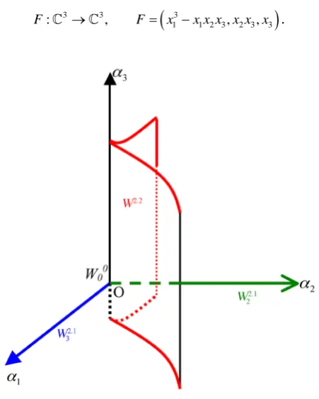
K F by smooth varieties (see Figure 2).

Remark 4.9. If K0

( )

F \SF is smooth, then we can define easily a stratification of

the set K0

( )

F ∪SF. But in general, K0

( )

F \SF is not smooth. We can check this

fact in the following example:

(

)

3 3 3

1 1 2 3 2 3 3

: , , ,

[image:10.595.261.487.380.662.2]

F  → F= x −x x x x x x .

Figure 2. The partition of K0

( )

F defined by Thom of the

polynomial mapping

(

3

)

1 1 2 3, 2 3, 3 1

Remark 4.10. In all examples in this paper and in [16], the set K0

( )

F ∪SF is pure

dimensional if F is dominant. So we can suggest the following conjecture:

Conjecture 4.11. If _F:_n→_n is a dominant polynomial mapping then the set

( )

0 F

K F ∪S is pure dimensional.

Notice that the above conjecture is not true in the case F is not dominant, as

shown in the following example:

(

)

3 3 2

1 2 3 2 3 1 3

: , , , .

F  → F= x −x x x −x x −x

5. The Homology and Intersection Homology of the Variety

V

F

In this section, we prove the principal results of the paper, which are the two following theorems.

Theorem 5.1. Let 2 2

:

F  → be a non-proper generic dominant polynomial

mapping. Then for any variety VF associated to F, we have

1) H V2

( )

F ≠0,

2) 2

( )

0

p F

IH V ≠ for any perversity p,

3) 2

( )

0

p F

IH V ≠ for some perversity p.

Theorem 5.2. Let : n n

(

3

)

F  → n≥ be a non-proper generic dominant poly-

nomial mapping. If

( )

1, ,

ˆ

Rank _i 1

i n

DF n

= ≥ −

 _ , where Fˆi is the leading form of Fi,

then for any variety VF associated to F, we have

1) H V2

( )

F ≠0,

2) 2

( )

0

p F

IH V ≠ for any (or some) perversity p,

3) 2 2

( )

0

p n F

IH − V ≠ , for any (or some) perversity p.

Before proving these theorems, we recall some necessary definitions and lemmas. Definition 5.3. A semi-algebraic family of sets (parametrized by ) is a semi-

algebraic set n

A⊂ ×, the last variable being considered as parameter.

Remark 5.4. A semi-algebraic set n

A⊂ × will be considered as a family para-

metrized by t∈. We write At, for “the fiber of A at t”, i.e.:

( )

{

}

: n: , .

t

A = x∈ x t ∈A

Lemma 5.5 ([1] lemma 3.1). Let β be a j-cycle and let _A⊂n_× be a com-

pact semi-algebraic family of sets with β ⊂At for any t. Assume that β bounds a

(

j+1

)

-chain in each A_t, t>0 small enough. Then β bounds a chain in A₀.

Definition 5.6 ([1]). Given a subset _X ⊂_n, we define the “tangent cone at

infinity”, called “contour apparent à l'infini” in [16] by:

( )

{

( )

(

]

( )

( )

_{( )}

0 0 1

0 0

: 0,1 such that : , semi algebraic,

lim , lim

n

t t t t

C X t t X

t t

t

λ η ε

η

η λ

η

− ∞

→ →

= ∈ ∃ + → −

 = ∞ =   

Lemma 5.7 ([2] lemma 4.10). Let

(

1, ,

)

:

n m

m

F = F  F  → be a polynomial

mapping and V be the zero locus of Fˆ:=

(

Fˆ1,,Fˆm

)

, where Fˆi is the leading form

of Fi. If X is a subset of n

subset of 1

( )

0,1

n

V

− _∩

 , where _ˆ 1

( )

0

V =F− .

Proof. (Proof of the Theorem 5.1).

The proof of this theorem consists into three steps:

+ In the first step, we use the Transversality Theorem of Thom (see [17], p. 34): if F

is non-proper generic dominant polynomial mapping, we can construct an adapted

(

2,p

)

-allowable chain in generic position providing non triviality of homology and

intersection homology of the variety VF, for any perversity p.

+ In the second step, we use the same idea than in [1] to prove that the chain that we create in the first step cannot bound a 3-chain in VF.

+ In the third step, we provide an explicit stratification of the singular set of VF, so

that the properties of the homology and the intersection homology of the set VF in

the theorem do not change for all the varieties VF associated to F.

a) Step 1: Let 2 2

:

F  → be a generic polynomial mapping, then dim_V_F =4 ([1], proposition 2.3). Assume that SF ≠ ∅. We claim that SF ∩K0

( )

F ≠ ∅. In fact, since F is dominant, then by the Theorem 2.11, we have dimSF =1. Moreover, since F is generic then dimK0

( )

F =1. Thanks again to the genericity of F, we have SF ∩K0

( )

F ≠ ∅. Let x0∈SF \K0

( )

F , then there exists a complex Puiseux arc

γ in _4_{, where}

( )

4

:D 0, , uzα ,

γ η → γ = +

(with α is a negative integer, u is an unit vector of 4 and D

( )

0,η a small

2-dimensional disc centered in 0 and radius η) tending to infinity in such a way that

( )

F γ converges to x₀. Then, the mapping h_Fγ , where h_F =

(

F,ψ₁,,ψ_p

)

(see the construction of the variety VF, Section 3) provides a singular 2-simplex in VF

that we will denote by c. We prove now the simplex c is

(

p, 2

)

-allowable for any

perversity p. In fact, since dim_S_F =1, the condition (see 2.8)

{ }

0

(

(

{ }

)

)

0=dim x =dim SF× 0_p ∩ c ≤ − +2 α pα,

where α =codim_S_F =2 holds for any perversity p since p₂=0.

Notice that VF \SF is not smooth in general. In fact, Sing

(

VF \SF

)

⊂K0

( )

F . Let us consider a stratum Vi of the stratification of K0

( )

F ∪SF defined in the Theorem

4.6 and denote β =codim_V_i. Assume that β ≥2, we can choose the Puiseux arc γ such that c lies in the regular part of VF\

(

SF×

{ }

0_q

)

, thanks to the genericity of F.

In fact, this comes from the generic position of transversality. So c is

(

p, 2

)

-

allowable. Hence we only need to consider the cases β =0 and β =1. Then:

1) If c intersects V_i: since x₀∈S_F \K₀

( )

F , then we have 0≤dim_

(

V_i∩c

)

≤1. Considering the condition

(5.8) dim_

(

V_i∩ c

)

≤ − +2 β p_β. We see that 2− +β p_β ≥1, for β =0 and β =1. So the condition (5.8) holds. 2) If c does not meet Vi, then the condition

(

)

holds always.

In conclusion, the simplex c is

(

p, 2

)

-allowable for any perversity p.

We can always choose the Puiseux arc such that the support of ∂c lies in the regular

part of VF\

(

SF×

{ }

0_p

)

and ∂c bounds a 2-dimensional singular chain e of

{ }

(

)

(

)

Reg VF\ SF× 0_p . So σ = −c e is a

(

p, 2

)

-allowable cycle of VF.

b) Step 2: We claim that σ cannot bound a 3-chain in VF. Assume otherwise, i.e.

assume that there is a 3-chain in VF, satisfying ∂ =τ σ. Let

{ }

(

)

(

)

(

)

1

: F F \ F 0 p ,

A =h− σ ∩ V S ×



{ }

(

)

(

)

(

)

1

: F F \ F 0 p .

B =h− τ ∩ V S × _

By definition 5.6, the sets C_∞

( )

A and C_∞

( )

B are subsets of 3

( )

0,1 . Observe

that, in a neighborhood of infinity, A coincides with the support of the Puiseux arc

γ. The set C_∞

( )

A is equal to 1_⋅a (denoting the orbit of _a∈2 under the action

of 1 on _2,

(

_{e ,}iη _z

)

_eiη_z). Let _V be the zero locus of the leading forms

(

1 2

)

ˆ_: ˆ ˆ_,

F = F F . Since F A

( )

and F B

( )

are bounded, then by lemma 5.7, the sets

( )

C_∞ A and C_∞

( )

B are subsets of V∩3

( )

0,1 .

For R large enough, the sphere 3

(

0,R

)

with center 0 and radius R in 4 is

transverse to A and B (at regular points). Let

(

)

(

)

3 3

: 0, , : 0, .

R R A R R B

σ =_ ∩ τ =_ ∩

Then σR is a chain bounding the chain τR. Considering a semi-algebraic strong

deformation retraction

[ ]

1

:W 0;1 a

Φ × → ⋅_{ , where} W is a neighborhood of 1⋅a

in 3

( )

0,1

 onto 1

a ⋅

 . Considering R as a parameter, we have the following semi-

algebraic families of chains: 1) : R

R

R σ

σ = , for R large enough, then σR is contained in W,

2) σR′ = Φ1

( )

σR , where Φ1

( )

x := Φ

( )

x,1 , x W∈ , 3) θR= Φ

( )

σR , we have ∂θR=σR′ −σR,

4) θR′ =τR+θR, we have ∂θR′ =σR′.

As, near infinity, σR coincides with the intersection of the support of the arc γ

with 3

(

)

0,R

 , for R large enough the class of σR′ in

1⋅_a

 is nonzero.

Let r=1R, consider r as a parameter, and let

{ }

σr ,

{ }

σr′ ,

{ }

θr as well as

{ }

θr′ the corresponding semi-algebraic families of chains.

Let us denote by 4

r

E ⊂ × the closure of θr , and set

(

{ }

)

4 0: 0

E =  × ∩E.

Since the strong deformation retraction Φ _{is the identity on} C_∞

( )

A ×

[ ]

0,1 , we see

that

( )

[ ]

(

)

1 3

( )

0 0,1 0,1 .

E ⊂ Φ C_∞ A × = ⋅ ⊂ ∩a V 

Let us denote by 4

r

E′ ⊂ × the closure of θr′, and set

(

{ }

)

4 0: 0

E′ =  × ∩E′.

Since A bounds B, then C_∞

( )

A is contained in C_∞

( )

B . We have

( )

3

( )

0 0 0,1 .

The class of σr′ in

1_⋅a

 is, up to a product with a nonzero constant, equal to the generator of 1

a ⋅

 . Therefore, since σr′ bounds the chain θr′, the cycle

1

a ⋅

 must bound a chain in θr′ as well. By Lemma 5.5, this implies that

1_⋅a

 bounds a chain in E0′ which is included in

( )

3

0,1

V∩ .

The set V is a projective variety which is an union of cones in 4. Since

dim_V ≤1, so dim_V ≤2 and dim_V∩3

( )

0,1 ≤1. The cycle 1

a ⋅

 thus bounds a chain in 3

( )

0 0,1

E′ ⊆ ∩V  , which is a finite union of circles, that provides a

contradiction.

c) Step 3: We prove at first the afirmation: If F is dominant, then F is generically

finite. Recall that F is generically finite if there exists a subset U⊂n in the target

space such that U is dense in n and for any a∈U , the cardinality of F−1

( )

a is

finite. To prove that F is generically finite, we do two steps:

+ Prove that

( ) ( )

n n F

F  =F  ∪S . In fact, by the definition of S_F (see (2.12)), it is

clear that

( )

n

( )

n F

F  ∪S ⊂F  . Take now a∈F

( )

n , then there exists a

sequence

{ }

n k

ξ ⊂ such that F

( )

ξk tends to a. If ξk tends to infinity, then a belongs to S_F. If ξ_k does not tend to infinity, assume that ξ_k tends to

n

ξ∈ . Since F is a polynomial mapping and hence is continuous, then F

( )

ξk

tends to F

( )

ξ . Moreover _n is a Hausdorff space, then _F

( )

ξ =_a. This implies

that

( )

n

a∈F  . Consequently, we have F

( ) ( )

n ⊂F n ∪SF . We conclude that

( ) ( )

n n

F

F  ⊂F  ∪S .

+ Indicate that there exists a dense subset U in the target space n in the target

space such that for any a∈U, the cardinality of F−1

( )

a is finite. In fact, let

\ .

n F

U = S

Since F is dominant, then by the Theorem 2.13, the dimension of S_F is n−1. Hence U is dense in the the target space n. With each a∈U, since a∉S_F, and

since F is a polynomial mapping, then the cardinality of F−1

( )

a is finite (see, for

example, the Proposition 6 of [11]). Then F is generically finite.

Since F is generically finite, then by the Theorem 4.6, there exists an explicit

Thom-Mather stratification of the set K0

( )

F ∪SF, which is compatible with the

Thom-Mather partition of K0

( )

F defined by [6] and is compatible with the Whitney

stratification of SF defined in [2]. In other words, there exists an explicit Thom-

Mather stratification of the variety VF, since K0

( )

F ∪SF is the singular part of the

set VF. We use this stratification to calculate the intersection homology of the variety

F

V . Since the obtained stratification is a Thom-Mather stratification, then it is a locally

topologically trivial stratification (Theorem 2.6). Hence the intersection homology of the variety VF does not depend on the stratification of VF (Theorem 2.9). Con-

sequently, the properties of the homology and the intersection homology of the variety

F

V in the theorem do not depend on the choice of the varieties associated to the

polynomial mapping F. 

We prove now the Theorem 5.2. Proof. (Proof of the Theorem 5.2).

mapping. Similarly to the previous proof, we have:

• _Since F is dominant, then by the Theorem 2.13, we have dim_S_F = −n 1. Moreover, since F is generic then dim_K₀

( )

F = −n 1. Thanks again to the genericity of F, we have S_F ∩K₀

( )

F ≠ ∅. Let x₀∈S_F\K₀

( )

F , then there exists

a complex Puiseux arc γ in _2n, where

( )

2

:D 0, n, uzα ,

γ η → γ = +

(with α is a negative integer and u is an unit vector of 2n) tending to infinity

such a way that F

( )

γ converges to x0. Since x0∈SF\K0

( )

F and F is generic, then we can choose the arc Puiseux γ in generic position, that means the simplex c

is

(

p, 2

)

-allowable for any perversity p.

• _{Now, with the same notations than the above proof, we have: Since}

( )

1, ,

ˆ

rank i 1

i n

DF n

= ≥ −

 _ then corank

( )

ˆi _{1, ,} 1 i n

DF

= ≤

 _ . Moreover since

( )

ˆ _{1, ,}

dim corank i

i n

V DF

=

=

  _ then dimV≤2 and

( )

2 1

dim_V∩ n− 0,1 ≤1. The

cycle 1⋅_a bounds a chain in 2 1

( )

0 0,1

n

E′ ⊆ ∩V  − , which is a finite union of

circles, that provides a contradiction.

Hence, we get the facts (1) and (2) of the theorem. Moreover, from the Goresky- MacPherson Poincaré Duality Theorem (Theorem 2.11), we have

( )

( )

, ,

2 2 4

p c q cl

F n F

IH V =IH ₋ V

where p and q are complementary perversities. Since the chain σ that we create

in the proof of the Theorem 5.1 can be either a chain with compact supports or a chain with closed supports, so we get the fact (3) of the theorem. 

Remark 5.9. The properties of the homology and intersection homology in the Theorem 5.1 and 5.2 hold for both compact supports and closed supports.

Remark 5.10. From the proofs of the Theorems 5.1 and 5.2, we see that the properties of the intersection homology in these theorems do not hold if F is not

dominant. The reason is that the Theorem 2.11 is not true if F is not dominant and

then the condition (5.8) does not hold. However, the properties of the homology hold even if F is not dominant. So we have the two following corollaries.

Corollary 5.11. Let _F:2→_2 be a non-proper generic polynomial mapping,

then H2

( )

VF ≠0.

Corollary 5.12. Let F:n→n

(

n≥3

)

be a non-proper generic polynomial

mapping. If

( )

1, ,

ˆ

Rank _i 1

i n

DF n

= ≥ −

 _ , where Fˆi is the leading form of Fi, then

( )

2 F 0 H V ≠ .

Remark 5.13. In the previous papers [1] and [2], the condition “F is nowhere

vanishing Jacobian” (see Theorems 3.3 and 3.4) implies F is dominant. Hence, the

condition “F is dominant” in the Theorems 5.1 and 5.2 guarantees the condition of

dimension of the set SF (see Theorem 2.13). Moreover, we need this condition in this

paper also to be free ourself from the condition K0

( )

F = ∅, since the condition of

dimension of SF when F is dominant also guarantees the (generic) tranversal

intersection homology of the variety VF when K0

( )

F ≠ ∅ in Theorems 5.1 and 5.2.

References

[1] Valette, A. and Valette, G. (2014)Geometry of Polynomial Mappings at Infinity via Inter-section Homology. Annales-Institut Fourier, 64, 2147-2163.

[2] Nguyen, T.B.T., Valette, A. and Valette, G. (2013) On a Singular Variety Associated to a Polynomial Mapping. Journal of Singularities, 7, 190-204.

[3] van den Essen, A.R.P. (1997) Polynomial Automorphisms and the Jacobian Conjecture.

Séminaires et Congrès, 2, 55-81. Société Mathématique de France.

[4] Brasselet, J.-P. (2015) Introduction to Intersection Homology and Perverse Sheaves. Insti-tuto de Matemática Pura e Aplicada, Rio de Janeiro.

[5] Borel, A., et al. (1984) Intersection Cohomology, Progress in Mathematics Vol 50. Birk-haüser.

[6] Thom, R. (1969) Ensembles et morphismes stratifiés. Bulletin of the American

Mathemati-cal Society, 75, 240-284.https://doi.org/10.1090/S0002-9904-1969-12138-5

[7] Whitney, H. (1965) Tangents to an Analytic Variety. Annals of Mathematics, 81, 496-549. https://doi.org/10.2307/1970400

[8] Goresky, M. and MacPherson, R. (1983) Intersection Homology II. Inventiones

Mathema-ticae, 72, 77-129.https://doi.org/10.1007/BF01389130

[9] Mather, J. (1970) Notes on Topological Stability. Miméographié, Harvard University, Cambridge, MA.

[10] Goresky, M. and MacPherson, R. (1980) Intersection Homology Theory. Topology, 19, 135-162.https://doi.org/10.1016/0040-9383(80)90003-8

[11] Jelonek, Z. (1993) The Set of Point at Which Polynomial Map Is Not Proper. Annales

Polo-nici Mathematici, 58, 259-266.

[12] Mostowski, T. (1976) Some Properties of the Ring of Nash Functions. Ann. Scuola Norm.

Sup. Pisa Cl. Sci., 3, 245-266.

[13] Trotman, D. (2005) Lectures on Real Stratification Theory. LATP-UMR 6632, University of Provence, Marseille.

[14] Nguyen, T.B.T. (2015) La méthode des façons. ArXiv: 1407.5239.

[15] Nguyen, T.B.T. (2016) Une stratification de Thom-Mather de l'ensemble asymptotique

d'une application : n n

F  → . ArXiv: 1611.01384.

[16] Nguyen, T.B.T. (2013) Étude de certains ensembles singuliers associés à une application polynomiale. Thèse, Université d’Aix Marseille. http://tel.archives-ouvertes.fr/