Estimates of the US Phillips curve with the general to specific method

Munich Personal RePEc Archive

Estimates of the US Phillips curve with

the general to specific method

Rao, B. Bhaskara and Paradiso, Antonio

University of Western Sydney, University of Rome La Sapienza

16 January 2011

Estimates of the US Phillips Curve

with the General to Specific Method

B. Bhaskara Rao

[email protected]

School of Economics and Finance, University of Western Sydney, Sydney (Australia)

Antonio Paradiso [email protected]

Department of Economics, University of Rome La Sapienza, Rome (Italy)

Abstract

This paper distinguishes between the long run and short run Phillips curve (PC) and uses the

micro theory based specification, with forward looking expectations, for the long run PC. The

long run and the implied short run dynamic equations are estimated in one step with the

general to specific method (GETS). Our approach has two distinct advantages. Firstly,

classical estimation methods can be used, irrespective of the stationarity properties of the

variables. Secondly, instead of arbitrarily adding the lagged inflation rate to the theory based

long run PC to capture persistence in inflation, our approach shows that persistence effects

can also be captured through the dynamic adjustment equations. This has an added advantage

because it offers a more flexible lag structure to estimate dynamic adjustments compared to

the partial adjustment process in the hybrid NKPC.

Keywords: US New Keynesian Phillips Curve, Forward looking expectations, Alternative

measures of the Driving Forces, GETS.

1. Introduction

Recent empirical studies of the new Keynesian Phillips curve (NKPC) have discussed several

issues concerning its specification and estimation. Two important controversial issues are the

relative importance of the backward and forward looking expectations and whether the output

gap or the share of wages is a satisfactory proxy for real marginal costs. Gali and Gertler

(1999) have augmented the micro-theory based new Keynesian Phillips curve (NKPC) and

forward looking expectations with the lagged inflation rate to analyse the relative importance

of the backward and forward looking expectations in the US inflation dynamics. With this

hybrid NKPC, Gali and Gertler (1999) found that although the coefficients of backward

looking expectations are significant, their effects are relatively smaller compared to forward

looking expectations. This result is interpreted by them as an indirect validation of the

micro-optimisation theory behind the NKPC. They also found that the share of wages is a better

proxy for marginal cost than the output gap.

However, Rudd and Whelan (2006, 2007) questioned these findings. They showed

that when a correctly specified NKPC, with model consistent rational expectations, is

estimated the coefficients of forward looking expectations are insignificant and inflation is

highly persistent. They did not find much difference in the proxies used for marginal costs. Rudd and Whelan’s findings have important policy implications because if inflation is highly persistent, that is backward looking expectations dominate inflation dynamics, then, the

effects of nominal shocks on the real variables will also persist and anti-inflation policies are

costly; see, for example, Guerron-Quintana (2011). Therefore, it is important to examine with

alternative procedures if backward or forward looking expectations dominate the dynamics of

inflation.

However, a neglected issue in this debate concerns the time series properties of its key

variables viz., the rate of inflation, variables used to proxy marginal cost and any survey

measures, if used, to proxy the expected rate of inflation. Recently Boug, Cappelen and

Swensen (2010) and Rao and Paradiso (2011) have examined the time series properties of

these variables with the US data but with different sample periods and found that they are

nonstationary in their levels and stationary in first differences. Therefore, they have estimated

the US NKPC with alternative time series methods of cointegration and error correction

method.

The justification for the present paper is as follows. There is more than one alternative

more efficient with better finite sample properties. For example, there are more than 100

alternative ways of testing for unit roots in some popular softwares like the EViews.

Therefore, different conclusions are possible with different tests, options and samples.1 For

example, in the US data used by Gali and Gertler (1999) for the period 1960Q1 to 1997Q4,

the standard unit root tests show that inflation rate has a unit root but the share of wages is

stationary. Pesaran and Shin’s (1999) ARDL method is popular with many applied workers to

estimate such relationships when the order of the variables is different. However, the ARDL

approach has some limitations in that the computed test statistics for cointegration may fall

into a substantial inconclusive range. Furthermore, the test statics are given for sample sizes

of 500 and above and their finite sample properties are not well known.

An alternative to the ARDL, and also other time series methods with all I(1) level

variables, is the general to specific method (GETS) of estimating the long and short run

relationships. GETS was originally developed in the1960s at the London School of

Economics (LSE) and David Hendry is its most ardent exponent and supporter.2 GETS takes

the view that dynamics is an empirical issue because economic theory is mostly silent on the

dynamics since theory is mainly concerned with establishing equilibrium relationships

between the levels of the variables. Therefore, dynamics should be estimated in a way

consistent with the underlying data generation process of the variables. GETS formulations

enable estimation of both the long run equilibrium and short run dynamic adjustment

parameters in one step. The theory behind the relationship is used to specify the long run part

of the specification in the levels of the variables and lagged changes in the variables are used

to specify the short run dynamics. Some time series econometricians, especially from North

America, were critical of GETS specifications because the order of the variables is different

in that level variables are generally I(1) and their differences are I(0), Hendry repeatedly

pointed out that such criticisms are incorrect because if the underlying economic theories are

valid for the specification of the long run relationships, then, the combination of the level

variables should also be stationary. Therefore, GETS specifications consist of only I(0)

variables and they can be estimated with the standard classical methods.3

1 It is not uncommon to find that many applied works devote proportionately a large amount of space to present

and discuss unit root test results with several options. 2

It existed as a oral tradition in the LSE undergraduate applied courses of the early 1960s before Sargan, Mizon

and Hendry gave more formal econometric foundations in the mid 1960s. 3

The implication of the above discussion to estimate the NKPC is follows. According

to GETS the NKPC can be estimated with a classical method, such as the GMM, as long as

the underlying micro theory on how firms set optimal product prices is valid. Therefore, this

paper illustrates the use of GETS to estimate the US NKPC. Our sample is for 1978Q1 to

2010Q2 and this choice is due to some constraints on the availability of data to proxy forward

looking expectations.

The rest of this paper is as follows. Section 2 examines specification issues and

empirical results are presented and discussed in Section 3. Section 4 concludes.

2. Specification

For the long run Phillips curve we shall use the following Gali and Gertler’s (1999)

specification, based on the optimisation model with forward expectations.

(1) ln ln ( ln 1)

>0; 1.

t t

P   S E P

 



    

wherelnPrate of inflation and Sshare of wages to proxy marginal cost. An alternative proxy for marginal cost is the well known output gap (GAP), measured as the difference

between the logs of actual and potential outputs. GETS formulation assumes that the

observed change in the dependent variable, in our case the rate of acceleration of inflation

2

( ln ),P is due to two reasons. Firstly, if in the previous period the actual rate of inflation did not fully adjust to its equilibrium rate in equation (1), inflation rate in the current period

changes to close partly this gap. Secondly, inflation rate may also change due to changes in

its determinants viz., wage share and the expected rate of inflation. Therefore, the GETS

specification of the NKPC, augmented with lags of the dependent variable to capture

persistence, is:

(2)





1 2

2

1 2

1 1

2

1 1 1

3 3 1 2

+ ln + +

ln ln ( ln ( ln )

( ln )

(0, )

n n

i t I j t j

i j

t t t t t

n

m t j t j t

m

P S

P P S E P

E P

N

 

  

 

 

 

 

  

  



 

      

  

The Gali and Gertler method of proxying forward looking expectations with the actual value

of the rate of inflation would cause serious estimation problems because of the presence of

both the current and lagged inflation rates on the right hand and especially when  is expected to be unity. The matrix of the coefficients will be singular and estimation breaks

down. Therefore, it is necessary to proxy the expected rate of inflation with some survey

based measure of the expected rate of inflation. Although in the USA there are four survey

based estimates of the expected rate of inflation, we selected the survey data of the University

of Michigan from 1978Q1 to 2010Q2 for two reasons. Firstly, Baghestani and Noori (1988) have shown that these are consistent with Pearce’s (1978) criteria of rationsal expectations. Secondly, consisten data without major revisions to the survey methods, are available from

1978Q1 for the Michigan survey. Denoting this as MICH, equation (2) can be specified as:

(3)





1 2 3

2

1 2 3

1 1 1

2

1 1 1

2

+ ln + +

ln ln ( ln )

(0, )

n n n

i t I j t j m

i j m

t t t t

t m t

P S

P P S MICH

MICH N

  

  



 

 

  

  



 

     

 







where MICH= University of Michigan’s forecast of the median rate of expected inflation four quarters ahead. Our inflation rate is measured with the core CPI and also with the

standard GDP deflator. Further details of the definitions of the variables and sources of data

are in the appendix.

3. Empirical Results

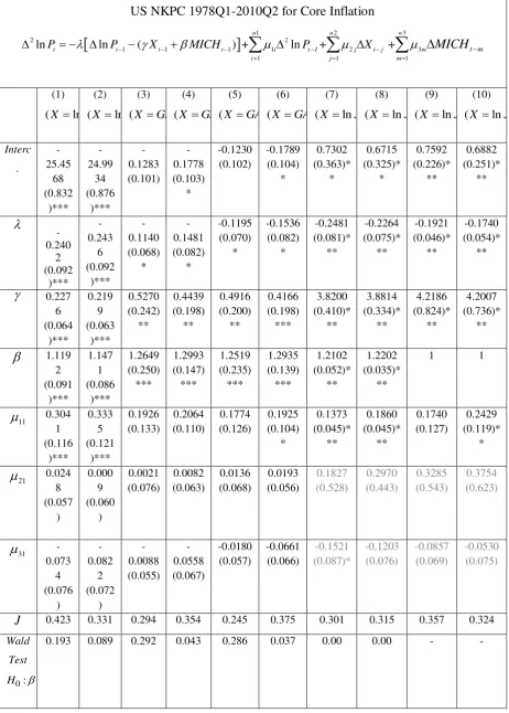
Equation (3) is estimated for the period 1978Q1 to 2010Q2 with GMM and with similar

instruments used by Gali and Gertler (1999). The results, with inflation measured with the

core CPI, are in Table 1. For convenience this table is split into two pages. In columns (1)

and (2) the driving force of inflation is proxied with the share of wages (ln ).S In column (1) estimates with the laged changes of the three variables is shown. In column (2) estimates the

instrument are reduced by dropping the spread between the short and long run interest rates

(SPREAD), to see how sensitive are the estimates to the choice of instruments. The estimates of the coefficients in column (2) are similar to those in column (1). We shall discuss these

are in columns (3) to (10). These proxies are four measures of the output gap (GAP1, GAP2, GAP3 and GAP) and the log of the probability of finding a job by newly unemployed

workers (lnJFP).

Output gap is the difference between the logs of actual and potential GDP and

potential GDP is computed in four alternative ways viz., as a liner trend (GAP1), as a

quadratic trend (GAP2), with the univariate unobserved component model (GAP3) and as HP filtered (GAP). However, results with GAP1 and GAP2 are unsatisfactory. The coefficient of

GAP1 turned out to be negative and of GAP2, although positive, is insignificant. To conserve space only results with GAP3 and GAP are reported in Table 1. The unsatisfactory results with GAP1 and GAP2, based on detrministic trends, may be due to shifts in the trend and

they may have been adequately captured by GAP and GAP3, with the stochastic trends.

Furthermore, a few alternative instrumental variables (shown in the notes to Table 1) are used

to check the sensitivity of the estimates.

In columns (1) to (8), where the four specifications are estimated with two alternative

sets of instrumental variables, the adjustment coefficienthas the expected negative sign and significant in all these estimates. Its absolute values ranged from 0.25 to 0.11 depending on

the selected driving force and instruments. However, its estimate is more sensitive to the

selected driving force than the instruments. The speeds of adjustment with both the wage

share and job finding probability are similar and faster than with estimates with the two gaps.

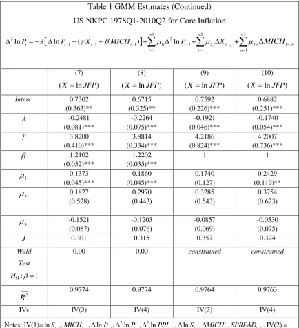
Estimates of the coefficient of the expected rate of inflation ( ) are closer in all estimates. Wald tests show that is not significantly different from the expected value of unity, at the 5% or 1% levels, with ln ,S GAPand GAP3,but exceeds unity in columns (7) and (8) withlnJFP. Therefore, these two equations are reestimated with the restriction that  1 and these estimates are in columns (9) and (10). In these constrained estimates there are only

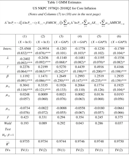
Table 1 GMM Estimates

US NKPC 1978Q1-2010Q2 for Core Inflation

(Notes and Columns (7) to (10) are in the next page)





2 2

1 1 1 1 2 3

1 1 1

ln ln ( ) + ln + +

n n n

t t t t i t I j t j m

i j m

t m

P  P_ X _ MICH_  P_  X_  MICH

  



     







(1)

(X ln )S

(2)

(X ln )S

(3)

(XGAP)

(4)

(X GAP)

(5)

(X GAP3)

(6)

(X GAP3)

Interc. -25.4568 (0.832)*** -24.9934 (0.876)*** -0.1283 (0.101) -0.1778 (0.103)* -0.1230 (0.102) -0.1789 (0.104)*  _-0.2402 (0.092)*** -0.2436 (0.092)*** -0.1140 (0.068)* -0.1481 (0.082)* -0.1195 (0.070)* -0.1536 (0.082)*  _0.2276 (0.064)*** 0.2199 (0.063)*** 0.5270 (0.242)** 0.4439 (0.198)** 0.4916 (0.200)** 0.4166 (0.198)***  1.1192 (0.091)*** 1.1471 (0.086)*** 1.2649 (0.250)*** 1.2993 (0.147)*** 1.2519 (0.235)*** 1.2935 (0.139)*** 11  0.3041 (0.116)*** 0.3335 (0.121)*** 0.1926 (0.133) 0.2064 (0.110) 0.1774 (0.126) 0.1925 (0.104)* 21  0.0248 (0.057) 0.0009 (0.060) 0.0021 (0.076) 0.0082 (0.063) 0.0136 (0.068) 0.0193 (0.056) 31  -0.0734 (0.076) -0.0822 (0.072) -0.0088 (0.055) -0.0558 (0.067) -0.0180 (0.057) -0.0661 (0.066)

J 0.423 0.331 0.294 0.354 0.245 0.375

Wald Test

0: 1

H  

0.193 0.089 0.292 0.043 0.286 0.037

___ 2

R 0.9755 0.9754 0.9744 0.9746 0.9748 0.9750

Table 1 GMM Estimates (Continued)

US NKPC 1978Q1-2010Q2 for Core Inflation





2 2

1 1 1 1 2 3

1 1 1

ln ln ( ) + ln + +

n n n

t t t t i t I j t j m

i j m

t m

P  P_ X _ MICH_  P_  X_  MICH

   

     







(7)

(X lnJFP)

(8)

(X lnJFP)

(9)

(X lnJFP)

(10)

(X lnJFP)

Interc. 0.7302 (0.363)** 0.6715 (0.325)** 0.7592 (0.226)*** 0.6882 (0.251)***  -0.2481 (0.081)*** -0.2264 (0.075)*** -0.1921 (0.046)*** -0.1740 (0.054)***  3.8200 (0.410)*** 3.8814 (0.334)*** 4.2186 (0.824)*** 4.2007 (0.736)***  1.2102 (0.052)*** 1.2202 (0.035)***

1 1

11  0.1373 (0.045)*** 0.1860 (0.045)*** 0.1740 (0.127) 0.2429 (0.119)** 21  0.1827 (0.528) 0.2970 (0.443) 0.3285 (0.543) 0.3754 (0.623) 31  -0.1521 (0.087) -0.1203 (0.076) -0.0857 (0.069) -0.0530 (0.075)

J 0.301 0.315 0.357 0.324

Wald

Test

0: 1

H  

0.00 0.00 constrained constrained

___ 2 R

0.9774 0.9774 0.9764 0.9763

IVs IV(3) IV(4) IV(3) IV(4)

Notes: IV(1)=lnS_t2,MICH_t2,lnP_t2,2lnP_t1,2lnPPI_t2,lnS_t1,MICH_t1,SPREAD_t2. IV(2) =

same as IV(1) without SPREAD_t2. IV(3) = same as IV(1) but with GAP3_t2 instead of SPREAD_t2.

IV(4) = same as IV(3) without GAP3_t2. Adjusted R-bar square is for the constrained version of the equation where the dependent variable is the rate of inflation. GAP1 has the wrong sign and GAP2 is not

In the dynamics part only the coefficients of the lagged dependent variable is

significant in all the estimates in columns (1) to (10), thus supporting our modification that

the effects of persistence are transitory and can be captured with the lagged dependent

variable. The coefficients of the lagged changes of the other two explanatory variables are

insignificant in all estimates. Deleting these insignificant variables did not result in any

significant changes to the estimates of the other parameters and are not reported to conserve

space. Alternative estimates with different sets of instrumental variables did not have any

significant effects and the Hansen Jtest shows that the instruments are over-identified. Furthermore, all our instruments are lagged values and are more likely to be independent of

the error terms of the equations. The pseudo R-bar squares are computed by re-estimating all

the equations by making the rate of inflation, instead of its change, as the dependent variable.

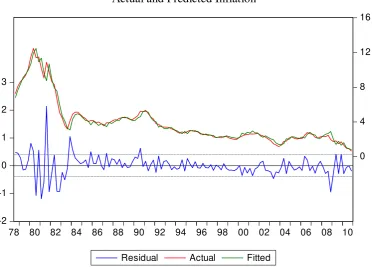
These are very high and Figure 1 shows a close relationship between the actual and predicted

rates of inflation with the equation in column (1). Plots with other estimates are similar and

not shown to conserve space. The minor over prediction of inflation around the late 2007 and

early 2008 is perhaps due to the financial crisis and its deflationary effects.

Figure 1

Actual and Predicted Inflation

-2 -1 0 1 2 3

0 4 8 12 16

78 80 82 84 86 88 90 92 94 96 98 00 02 04 06 08 10

On the basis of these results we may conclude: (a) the optimisation theory underlying

the NKPC, with forward looking expectations, is supported by our estimates with alternative

variables to proxy the driving force of inflation and marginal cost. In other empirical studies

one or another of these measures had a wrong or insignificant coefficient. However, it should

be noted that our estimates with gap measures with deterministic trends are also found to be

unsatisfactory; (b) the expectations hypothesis is validated by our results and (c) our

assumption that persistence effects are transitory is supported by the results in that the

coefficients of the lagged dependent variable are all significant. However, these persistence

effects are not as high as in other empirical studies and their estimates are sensitive to the

selected proxy for the driving force.

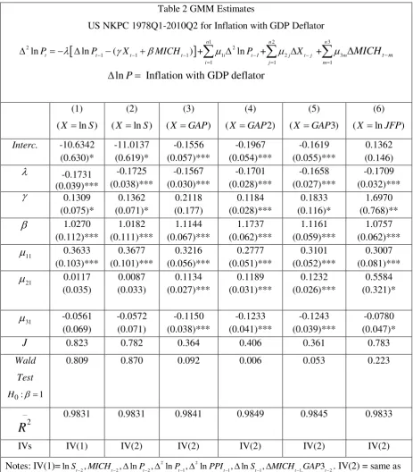
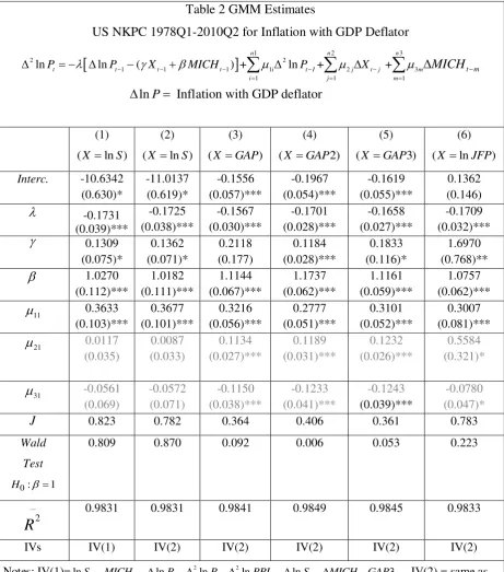
These above findings are further supported by the results in Table 2 where inflation is

measured with the GDP deflator. The coefficient of GAP2, where potential output is

measured with the quadratic time trend, is significant now but the Wald test rejected the null

that  1. Estimates of the adjustment coefficients are all significant and closer than their estimates in Table 1. They imply that about 15% to 17% adjustment in inflation towards its

equilibrium rate takes place in one quarter.

Estimates of  and the persistence coefficient ₁₁,with alternative measures of the driving force, are also much closer in Table 2 than in Table 1. The null that  1 _{is not} rejected by the Wald test in all but with GAP2 in column (4). Estimates of the persistence

coefficients ranged from about 0.28 (column (4)) to 0.37 (column (2)). All the estimates of

the coefficients are less sensitive to the selected instruments and the instruments are

Table 2 GMM Estimates

US NKPC 1978Q1-2010Q2 for Inflation with GDP Deflator





2 2

1 1 1 1 2 3

1 1 1

ln ln ( ) + ln + +

ln Inflation with GDP deflator

n n n

t t t t i t I j t j m

i j m

t m

P P X MICH P X MICH

P  _  _  _  _  _                







(2) (X ln )S

(3) (X GAP)

(4) (X GAP2)

(5) (X GAP3)

(6) (X lnJFP)

Interc. -10.6342 (0.630)* -11.0137 (0.619)* -0.1556 (0.057)*** -0.1967 (0.054)*** -0.1619 (0.055)*** 0.1362 (0.146)  _-0.1731 (0.039)*** -0.1725 (0.038)*** -0.1567 (0.030)*** -0.1701 (0.028)*** -0.1658 (0.027)*** -0.1709 (0.032)***  0.1309 (0.075)* 0.1362 (0.071)* 0.2118 (0.177) 0.1184 (0.028)*** 0.1833 (0.116)* 1.6970 (0.768)**  1.0270 (0.112)*** 1.0182 (0.111)*** 1.1144 (0.067)*** 1.1737 (0.062)*** 1.1161 (0.059)*** 1.0757 (0.062)*** 11  0.3633 (0.103)*** 0.3677 (0.101)*** 0.3216 (0.056)*** 0.2777 (0.051)*** 0.3101 (0.052)*** 0.3007 (0.081)*** 21  0.0117 (0.035) 0.0087 (0.033) 0.1134 (0.027)*** 0.1189 (0.031)*** 0.1232 (0.026)*** 0.5584 (0.321)* 31  -0.0561 (0.069) -0.0572 (0.071) -0.1150 (0.038)*** -0.1233 (0.041)*** -0.1243 (0.039)*** -0.0780 (0.047)*

J 0.823 0.782 0.364 0.406 0.361 0.783

Wald

Test

0: 1

H  

0.809 0.870 0.092 0.006 0.053 0.223

__

2

R

0.9831 0.9831 0.9841 0.9849 0.9845 0.9833

IVs IV(1) IV(2) IV(2) IV(2) IV(2) IV(2)

Notes: IV(1)= 2 2

2 2 2 1 1 1 1, 2

lnS_t ,MICH_t ,lnP_t , lnP_t, lnPPI_t,lnS_t,MICH_t GAP3_t . IV(2) = same as

4. Conclusions

In this paper we have used the LSE and Hendry GETS approach to specify and estimate the

US NKPC. Some new features of our approach, among which the most important ones are a

distinction between the long run theory based expectations augmented Phillips curve and the

introduction of persistence effects into the dynamics of this relationship. Our major findings

are that alternative proxies for the inflation driving force are all satisfactory with the

exception of gaps estimated with the deterministic trends; the theory based NKPC with the

forward looking expectations is sound and our results support this; the long run Phillips curve

is vertical and therefore the real effects of nominal shocks are significant only during the

transition of the economy between its equilibrium states and the duration of this transition

period seems to be shorter than estimates with arbitrarily adding the lagged inflation rate to

the NKPC. However, more reliable estimates of the duration of this transition period would

be useful and can be estimated by simulating the effects of nominal shocks with an aggregate

demand and supply model in which the NKPC plays an important role. Therefore, our

conclusion on the duration of the transition period should be treated with caution.

Data Appendix

Definitions and Data Source: 1978Q1 – 2010Q2

Variable Definition Source

lnP

 _{Measured as}

4

ln t

t p p

 

  using core CPI. Consumer Price Index (All Items Less Food and Energy), Index 1982-1984=100.

In Table 2 we measure inflation using GDP deflator (Index 2005=100).

research.stlouisfed.org/f red2/categories/9

research.stlouisfed.org/f red2/categories/21

lnPPI

 _{Measured as}

4

ln t

t ppi ppi

 

  using Producer Price Index: Finished goods (Index 1982 = 100).

research.stlouisfed.org/f red2/categories/31

, 1, 2, 3 GAP GAP

GAP GAP

GAP = output gap (Nonfarm business sector, index 1992 = 100) using the Hodrick-Prescott filter with a smoothing parameter of 1600.

GAP 1 = output gap (Nonfarm business sector, index 1992 = 100) using a linear trend.

GAP 2 = output gap (Nonfarm business sector, index 1992 = 100) using a quadratic trend.

GAP 3 = output gap (Nonfarm business sector, index 1992 = 100) using univariate unobserved component models technique.

research.stlouisfed.org/f red2/categories/2

lnS Labour’s Share of Income (Nonfarm Business

Sector, Index 2005=100) expressed in natural log and multiplied for 100.

www.bls.gov/data

lnJFP Log of Job Finding Probability. Constructed from the number of unemployed workers (U_t), the

number of short term (1 month, U_tS_1) unemployed workers and the number of unemployed workers next month (U_t1) according to Shimer (2005):

1 1

1

s

t t

t

U U

JFP

U

  

 

www.bls.gov

SPREAD Difference between 10-Year Treasury constant maturity rate and Federal Fed Funds.

research.stlouisfed.org/f red2/categories/22





t

t t

MICH

E P_

 

Median expected price change next 12 months, Survey of Consumers.

References

Baghestani, H. and Noori, E. (1988), “On the rationality of the Michigan monthly survey of inflationary expectations”, Economics Letters, 27, 333-315.

Boug, P., Cappelen, A. and Swensen, A. R. (2010), “The new Keynesian Phillips curve revisited”, Journal of Economic Dynamics and Control, 34, 858-874.

Gali, J. and Gertler, M. (1999), “Inflation dynamics: A structural econometric analysis”,

Journal of Monetary Economics, 44, 195-222.

Guerron-Quintana, P. A. (2011), “The implications of inflation in an estimated new Keynesian model”, Journal of Economic Dynamics and Control, doi:10.1016/j.jedc. 2011.01.008.

Pearce, D. K. (1978), “Comparing survey and rational measures of expected inflation: Forecast performance and interest rate effects”, Journal of Money, Credit and Banking, 11, 446-456.

Pesaran, H. M., and Shin, Y. (1999), “Autoregressive distributed lag modelling approach to

cointegration analysis, Chapter 11, in: Storm, S. (ed.), Econometrics and Economic Theory in the 20th Century: The Ragnar Frisch Centennial Symposium, Cambridge University Press.

Rao, B. B. (2007), “Estimating short and long run relationships: A guide for the applied economist”, Applied Economics, 39, 1613-1625.

Rao, B. B., Singh, R. and Kumar, S. (2010), “Do we need time series econometrics?”,

Applied Economics Letters, 17, 695-697.

Rao, B. B. and Paradiso, A. (2011), “Time series estimates of the US NKPC”,

Rudd, J. and Whelan, K. (2006), “Can Rational Expectations Sticky-Price Models Explain Inflation Dynamics?”, American EconomicReview, 96 (March), 303–320.

Rudd, J. and Whelan, K. (2007), “Modelling inflation dynamics: A critical review of recent research”, Journal of Money, Credit and Banking, 39, 155–170.

Shimer, R. (2005), “Reassessing the Ins and Outs of unemployment”, NBER Working Paper

Table 1 GMM Estimates

US NKPC 1978Q1-2010Q2 for Core Inflation





2 2

1 1 1 1 2 3

1 1 1

ln ln ( ) + ln + +

n n n

t t t t i t I j t j m

i j m

t m

P  P_ X _ MICH _  P_  X _  MICH

  



     







(1)

(X lnS

(2)

(X lnS (3)

(X GA )

(4)

(X GA )

(5)

(X GA

(6)

(X GA (7)

(X lnJ (8)

(X lnJ (9)

(X lnJ (10)

(X lnJ

Interc . -25.45 68 (0.832 )*** -24.99 34 (0.876 )*** -0.1283 (0.101) -0.1778 (0.103) * -0.1230 (0.102) -0.1789 (0.104) * 0.7302 (0.363)* * 0.6715 (0.325)* * 0.7592 (0.226)* ** 0.6882 (0.251)* **  -0.240 2 (0.092 )*** -0.243 6 (0.092 )*** -0.1140 (0.068) * -0.1481 (0.082) * -0.1195 (0.070) * -0.1536 (0.082) * -0.2481 (0.081)* ** -0.2264 (0.075)* ** -0.1921 (0.046)* ** -0.1740 (0.054)* **  0.227 6 (0.064 )*** 0.219 9 (0.063 )*** 0.5270 (0.242) ** 0.4439 (0.198) ** 0.4916 (0.200) ** 0.4166 (0.198) *** 3.8200 (0.410)* ** 3.8814 (0.334)* ** 4.2186 (0.824)* ** 4.2007 (0.736)* **  1.119 2 (0.091 )*** 1.147 1 (0.086 )*** 1.2649 (0.250) *** 1.2993 (0.147) *** 1.2519 (0.235) *** 1.2935 (0.139) *** 1.2102 (0.052)* ** 1.2202 (0.035)* **

1 1

11  0.304 1 (0.116 )*** 0.333 5 (0.121 )*** 0.1926 (0.133) 0.2064 (0.110) 0.1774 (0.126) 0.1925 (0.104) * 0.1373 (0.045)* ** 0.1860 (0.045)* ** 0.1740 (0.127) 0.2429 (0.119)* * 21  0.024 8 (0.057 ) 0.000 9 (0.060 ) 0.0021 (0.076) 0.0082 (0.063) 0.0136 (0.068) 0.0193 (0.056) 0.1827 (0.528) 0.2970 (0.443) 0.3285 (0.543) 0.3754 (0.623) 31  -0.073 4 (0.076 ) -0.082 2 (0.072 ) -0.0088 (0.055) -0.0558 (0.067) -0.0180 (0.057) -0.0661 (0.066) -0.1521 (0.087)* -0.1203 (0.076) -0.0857 (0.069) -0.0530 (0.075)

J 0.423 0.331 0.294 0.354 0.245 0.375 0.301 0.315 0.357 0.324

Wald

Test

0: 1

H 

___ 2 R

0.975

5

0.975

4

0.9744 0.9746 0.9748 0.9750 0.9774 0.9774 0.9764 0.9763

IVs IV(1) IV(2) IV(1) IV(2) IV(1) IV(2) IV(3) IV(4) IV(3) IV(4)

Notes: IV(1)=lnS_t2,MICH_t2,lnP_t2,2lnP_t1,2lnPPI_t2,lnS_t1,MICH_t1,SPREAD_t2. IV(2) = same as

IV(1) without SPREAD_t2. IV(3) = same as IV(1) but with GAP3_t2 instead of SPREAD_t2. IV(4) = same as

IV(3) without GAP3_t2. Adjusted R-bar square is for the constrained version of the equation where the

dependent variable is the rate of inflation. GAP1 has the wrong sign and GAP2 is not statistically significant and

Table 2 GMM Estimates

US NKPC 1978Q1-2010Q2 for Inflation with GDP Deflator





2 2

1 1 1 1 2 3

1 1 1

ln ln ( ) + ln + +

ln Inflation with GDP deflator

n n n

t t t t i t I j t j m

i j m

t m

P P X MICH P X MICH

P  _  _  _  _  _                







(2) (X ln )S

(3) (X GAP)

(4) (X GAP2)

(5) (X GAP3)

(6) (X lnJFP)

Interc. -10.6342 (0.630)* -11.0137 (0.619)* -0.1556 (0.057)*** -0.1967 (0.054)*** -0.1619 (0.055)*** 0.1362 (0.146)  _-0.1731 (0.039)*** -0.1725 (0.038)*** -0.1567 (0.030)*** -0.1701 (0.028)*** -0.1658 (0.027)*** -0.1709 (0.032)***  _0.1309 (0.075)* 0.1362 (0.071)* 0.2118 (0.177) 0.1184 (0.028)*** 0.1833 (0.116)* 1.6970 (0.768)**  1.0270 (0.112)*** 1.0182 (0.111)*** 1.1144 (0.067)*** 1.1737 (0.062)*** 1.1161 (0.059)*** 1.0757 (0.062)*** 11  0.3633 (0.103)*** 0.3677 (0.101)*** 0.3216 (0.056)*** 0.2777 (0.051)*** 0.3101 (0.052)*** 0.3007 (0.081)*** 21  0.0117 (0.035) 0.0087 (0.033) 0.1134 (0.027)*** 0.1189 (0.031)*** 0.1232 (0.026)*** 0.5584 (0.321)* 31  -0.0561 (0.069) -0.0572 (0.071) -0.1150 (0.038)*** -0.1233 (0.041)*** -0.1243 (0.039)*** -0.0780 (0.047)*

J 0.823 0.782 0.364 0.406 0.361 0.783

Wald

Test

0: 1

H 

0.809 0.870 0.092 0.006 0.053 0.223

__

2

R

0.9831 0.9831 0.9841 0.9849 0.9845 0.9833

IVs IV(1) IV(2) IV(2) IV(2) IV(2) IV(2)

Notes: IV(1)= 2 2

2 2 2 1 1 1 1, 2

lnSt ,MICHt ,lnPt , lnPt, lnPPIt,lnSt,MICHt GAP3t . IV(2) = same as