A Lemma on Almost Regular Graphs and an Alternative Proof for Bounds on γt (Pk □ Pm)

(1)

A Lemma on Almost Regular Graphs and an Alternative

Proof for Bounds on



_t



P

_k



P

_m



Paul Feit

Department of Mathematics, University of Texas of the Permian Basin, Odessa, USA Email: feit_p @utpb.edu

Received July 16, 2013; revised August 10, 2013; accepted September 3, 2013

Copyright © 2013 Paul Feit. This is an open access article distributed under the Creative Commons Attribution License, which per- mits unrestricted use, distribution, and reproduction in any medium, provided the original work is properly cited.

ABSTRACT

Gravier et al. established bounds on the size of a minimal totally dominant subset for graphs . This paper offers

an alternative calculation, based on the following lemma: Let

k m

PP

,

k r so k3 and r2. Let H be an -

regular finite graph, and put . 1) If a perfect totally dominant subset exists for , then it is minimal; 2) If

and a perfect totally dominant subset exists for , then every minimal totally dominant subset of must be

perfect. Perfect dominant subsets exist for when and satisfy specific modular conditions. Bounds for

, for all follow easily from this lemma. Note: The analogue to this result, in which we replace “totally

dominant” by simply “dominant”, is also true.

r

k

GPH G

> 2

r



t Pk



G G

k

PC_n



k n

m P

 k m,

Keywords: Domination; Total Domination; Matrix; Linear Algebra

1. Introduction

Let be a graph. In this paper, each

edge of a graph must have two different endpoints; also, two vertices may be linked by at most one edge. A subset

Z of vertices is said to totally dominate G if every vertex

of G has a neighbor in Z. We say Z perfectly totally

dominates if every vertex has exactly one neighbor in Z.

Next, suppose that G is finite. In this case, we say a

totally dominant subset Z is minimal if

   



,

G V G E G

Z is the

smallest size possible among all dominant subsets. This

minimal size is denoted by t

 

G .

For , we say that a graph G is r-regular if every

vertex is the endpoint of exactly r edges. Suppose G is

regular. A subset Z which perfectly totally dominates is

clearly minimal. If a perfect dominant set does not exist,

we can search for minimality among dominant subsets Z

by counting “overlaps”. That is, for each

r

 

vV G

v

, let

t be the number of neighbors of which lie

in Z, minus 1. If



, ,G Z



ol v

1

Z and Z₂ are two totally dominant

subsets, then Z1 < Z2 happens if and only if the sum

of Z1-overlaps is strictly less than the sum of Z2-

overlaps.

These elementary links between minimality, perfection

and overlaps may fail if G is not regular. For arbitrary

theorists, a challenge is to specific assertions that apply to a broad family of graphs.

The following conventions

graphs, all sorts of behavior is possible. For graph

will be used here.

(1a) For k, k2, let Pk, the k -path be the

graph whose ce the numbers 2, , k, and

whose edges are links from i to i1 for each i<k

verti s are 1,

1 .

There is an infinite member of family: Inte

as a graph in which edges consist of links from i

1

i

this rpret 

to

 for all i.

b) Let >k

(1 The graph consisting of plus an

ed

) Fo and

2 . n 1 an

r G

k

P

is

ge betwee d k called the k-cycle. It denoted

by Ck.

(1c H graphs, the product graph

G H is de ed asfin follows. The set of vertices



H



is

V G V G

   

V H . Two vertices



x y₁, ₁



and



x y2, 2



r

ar edge if and only if

 ei 2

e linked by an

the x1x and y y1 2 is an edge of H, or

 x x_{1 2} is an edge of G and y₁ y₂.

For example, for k n, , P_kP_n is the familiar

k n grid map. A pro a aths and circuits

is called a grid graph.

A product of n copies of

duct of list of p

by 

 corresponds to the set

n_{with the “Ma hatten metric” notion of the edge: two}

les



tup

n



x1, , xn



and



y1, , yn



are linked if and

(2)

j j

x  y for all ji.

Tiling is the route that Gravier [1] takes in computing

t

 for grid graphs. The program begins with the work

herself, Molland and Payan [2] on the tiling question. The solution generates perfectly dominant subsets on

n

 . Now, finite grid graphs can be interpreted as rec-

ular subsets, or (for products with Cn factors) as

such subsets with some “opposed” sides i ntified. Do- mination becomes a problem of refining the patterns at the edges.

Our curr by

tang

do

nu

de

ent work exploits the abundance of perfect

minations on graphs GPkCn. A calculation with

matrices leads to a lower t

 

G that can only

be attained by a perfectly totally do t subset. Once

we classify which indices k n, admit perfect domi-

nations, an elementary trick ides upper and lower

bounds for all graphs PkCn. The bounds here do not

improve on the earlier w t are almost as narrow.

Suppose H is a finite r-regular graph for some natural

bound on

prov

ork, bu

minan

mber r, and put GPkH for k3. Then the

majority of vertices of G have a degree r2. The

vertices of the degree r1 form two conn sub-

graphs. A crude bound for minimal totally dominant

subset of G is

ected a



2



k H r . However, this bound is too

low by a positive number times H .

We find a subtler minimal bound usin he

t subset is minimal, and

bset cannot have fewer members

is odd, if a perfect totally e

nclusions follow from a formula which, for Z a

g matrices. T co

as

tha

do

tot

mputation also shows that (2a) A perfect totally dominan sumes the bound;

(2b) A minimal su n a perfect subset; and

(2c) Unless r2 and n

minant subset exists, th n every minimal subset is perfect.

The co

ally dominant subset, determines Z is a sum over

 

vV G of ol v Z G_t



, ,



_j , where each _j is a

w j of v.

Remark. A variation on total d inati n

non-zero

do

1.1. Sa

weight associated to ro

om o is (simple)

d v has no neighbors in Z, or

Z.

rfect

mple Perfect Behavior

ts: first, exhibit a sub-

ite. Id

mination. A subset dominates (non-totally) if each

vertex v either has a neighbor in Z or belongs to Z. A

dominant subset Z is perfect (non-totally) if for each

vertex v, either

(3a) vZ an

(3b) vZ and v has exactly one neighbor in

Our theory implies that, in this context, if a pe minant subset exists, it is minimal and every minimal dominant subset is perfect.

A proof of minimality has two par

set; then prove no smaller totally dominant subset can exist. The examples here are drawn from Gravier [1].

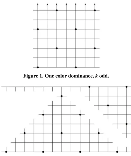
Assume n is even. In this case, PkCn is bipart

entify Cn with  n in the stan way. We can

“color” the vertices: we say

 

i j, (where j is read

mod

dard

 

n ) is black if i j is even and white if i j

is od hen every edg ks a black vertex with a w

one. If Z dominates PkCn, then the set of black

members of Z dominates all white vertices, and the white

vertices of Z dominate all the black. Consequently, a

minimal dominant subset is a disjoint union of two minimal “color” dominant subsets; each a subset of one color vertices that dominates all vertices of the other color. Furthermore, the “shift by 1” automorphism of

k k

PC identifies the sets of different colored vertices.

re 1 shows a pattern of vertices of one color

d. T

igu

us

e lin hite

.

stead,

F

Pr

as

ovided that k is odd, this pattern will totally domi-

nate all vertices of the opposite color.

If k is even, this pattern does not quite work. In

ill trated in Figure 2 for k8, one can build a

pattern by taking triangular wed of the first pattern,

and pairing them with a skew reflection. The latter

pattern can be repeated throughout PkCn provided

that

ges





2 k1 divides n.

The contribution of his pat per is a

set

n alternate construction of a lower bound. The bound is met for these perfect subsets. Next, using these subsets, one can estab-

lish a general upper bound for PkPm for all m.

1.2. A Tie with Perfection

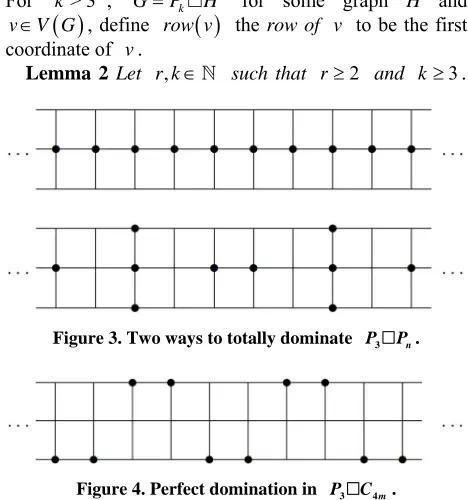
Gravier [1] proves that the Z consisting of the

middle row of P3Pn, for any n, s a minimal totally

[image:2.595.310.534.458.725.2]

dominant subset. Obviously, this choice of minimal i

Figure 1. One color dominance, k odd.

(3)

For each integer 1 j k, put

subset produces many overlaps. By rotating 3 3 blocks,

we can produce other minimal dominant se th fewer

overlaps, as in Figure 3. Furthermore, if n is a multiple

of 4, there is a variation which is a perfect total

domination of P3Cn, as in Figure 4. The flexibility in

the number of s which are dominated by more

than one member of

ts wi

vertice

Z reflects the presence of vertices

of two degrees, namely 3 and 4.

In this example, the size of a minimal, imperfect

to

1.3. Weights

ts of theorems based on series.

tally dominant subset “ties” the size of a perfect totally dominant set. Can a minimal subset be smaller than a perfect one? We prove that a tie is rare, and that beating is impossible.

We have two se

Definition 1 Let r be a real number. Let 

 

r



ai

be the set of infinite sequences of real numbers



_i_₀ such that

1 2 1, i i i .

i a ra_ a_

   

Clearly, 

 

r



₁ i i



 

.

is a real vector space, and the fu

real, let i be the unique member of nction



a



a a,



is a linear isomorphism from it onto 

For

0 1

2

r i

 

r,

 

r s ch that and 

 

r,1 1. Observe

 

r, 2 r

  .

In 

that

th

u

e o

 

r,0 0

 

g section, we def

penin ined the overlap function



, ,



t v G Z for totally dominant subsets Z of a graph G.

or G a graph and Z a dominant (but possibly

not totally) subset, and vV G

 

, let ol v G Z



, ,



be



, ,



t

ol v G Z if vZ an G Z,  Z ol

In addition, f

d ol vt



,



1 if v .

, G P H f h H

vV efine the row of v to be the first

of v. Lemma 2 L t

For k> 3

 

G , d

coordinate

k

 

row

or som

 

v e grap and

[image:3.595.54.288.484.734.2]

e r k,  such that r2 and k3.

Figure 3. Two ways to totally dominate P3Pn.

Figure 4. Perfect domination in P3C4m.





1

, j

r k

   



 

1 1 , 1

1 , .

j

k j

r k j

r j







     

 

For each 1 j k,

0

(4a)  j , and

(4b)  j 0 if and only if is odd and

is

fer to

2

r , k j

even.

We re 1, ,k as the weight system for para-

m

ition 3 Let eters r k, .

Defin r k,  such that r2 and

3

 . Let 1, , k

k   weight system r k, .

let 1,

be the for

Also,  ,k be the weight system for parame

1,

r k

ters

 . D



efine

 

 



   



 



1

2

2 2 , 1 2 , 1 2

, .

2 , 1

k

rk k r k r k

r k

r r k

 







    



 

Suppose H is an r-regular graph, and put n H

and GPkH. Define two functions on ZV

 

G :

 

Z  ol v Z G



, ,



 _{ }  

 





   

row

score

score , ,

t t v

v V G

t v

v V G

Z ol v Z G v



 



Theorem 4 Assume the hypothesis and construction of Lemma 2 and Definition 3. Let H be a finite graph, and put n H and GPkH.

(A) If Z V

 

G is totally dominant, then

 

_,

_

score

_{ }

t

 

Z

_

_.

2 , 1

Z n r k

r r k





 

 

(B) If ZV G

 

is dominant, then



1,



_

score

_{ }

 

Z

_

.

3 1, 1

Z n r k

r r k





  

  

A trivial consequence of this theorem and the pre- ce

ume the hypothesis of Theorem 4.

ding lemma is:

Corollary 5 Ass

(A) Suppose r3. If Z Z1, 2 are totally dominant subsets of G, then

 

1 < 2 scoret 1 < scoret 2 .

Z Z  Z Z

(B) If Z Z1, 2 are dominant subsets of G, then

 

1 2



score < score



. 1 < 2

Z Z  Z Z

2. Modeled with Matrices

linear algebra model. Our results are based on a simple

For convenience,

(5) For k, let Ind

  

k  1, , k



.

Notation 6. Let k. We identify the real vector

space _k_{with leng}_th _{olumn vectors. We use trans-}

(4)

pose notation to write these horizontally:

z

 1 T

1

( , , ) for k .

k

z z

z

       

 

For each 1 i k, let _i

k

nal

be the projection function

from each v z, , z



to its i-coordinate zi.

Also define a linear f _k _

k

ector



1

unctio

 

1

πi .

i

sum z z





We denote the zero vector by

d let H be a finite,

ˆ0. , a

In what follows, let k r,  n

r-regular graph. Put G .

For

 

k

P H

 

Z V G , define the row ount vector c z for Z to

be in

in the th u



z₁, , z_k



T which z_i is the number of members

of Z i- row. Obvio sly, sum z

 

 Z .

Now sup ose p Z V G

 

totally dominates, and let



z, ,z



 ₁  _k be ount vector. Let 1 i k

z its row c   .



, ,



t

l v Z G over all v in the i-th r

The sum of o ow, plus

H , equals

rz1 2

1 1

1

, for 1,

, for 1 1,and

, for .

i i i k k

z i

z rz z i k

z rz i k

 



 

    

 

(6)

In particular,

lly dominates, then each of these ex- pr

(7a) If Z tota

essions must be  H , and

(7b) If Z perfectly totally dominates, then each of these

expressions must equal H .

If we replace totally domination with simple domi-

na

ivate r next definition.

t be a na

tion, the analogous assertions hold after the r terms

in (6) are changed to r1.

These remarks mot ou

Definition 7 Let r be a real number and le k tural number > 1. Define L r k

 

, to be the k k matrix such that

 

 

,

if ,

, Ind , , 1 if is 1 or 1

0 otherwise.

i j

r i j

i j k L r k i j

 



    

 

,

Note that L r k

 

, hese pa

is symmetric.

Also, for t rameters, define M r k

 

, to be the

Note that the case is covered in both parts of this conditional definition.

atrix

k k matrix such that

 

, Ind ,

i j k

 

,



_

 

_{ }



_

, , 1 if ,

,

, , 1 if .

i j

r i r k j i j

M r k

r j r k i j i

 



     



  _ _ _{ } _



is essentially

 

1

,

r k L  .

3. Relevant Sequences

convexity for functions of a

i j

As we shall see, the m M r k

 

,

There is a discrete analogy to

single real variable. We recall some basics.

Definition 8 Let

 

ai i ₀ 

 be a sequence of real num- bers, starting at index We say that the sequence is convex if

0.

1 1

, i i i i .

i a a a a

    

We say a

the sequence isstrictly convexif

1 > 1

i ai aiai for each i.

 

ai ₀

Lemma 9 Let _i_ be a convex sequence. For

,v u ,

0 .

u v u v

a a a a

Moreover, au v auava0 ch that

if and only if there is a number t su



uv



, ai t ai1 . Ind

i

 

Proof.

ge

We may interchange u and v without loss of

nerality. Hence, assume uv. For each i, put

1

i i i

b  a a . Then

 

bi _i₁



 is a weakly increasing se-

quence. Then



 







0 0 0

1 1 1

0

1 1

0 1

1 1

0 1

1

u v

u v u v

i i i

v v

u v u v u i i

i i

v v

u v u v u v j i

j i

v

u v u v u v i i i

a a a a

b b b

a a a a b b

  

 

 

   

 

   



  

     

_ _{ } _{ } _

     

   

    _ _{ } _

   

   

    _ _{ } _

 

 

    _  _

 



u v 

Obse

a a 

(8)

rve that



 

2



1

i i u v v i

1

u    v     0 .

For eac fo

h index i in the last sum, the term has the

rmat bpbq where >p q. Therefore

0 0.

u v

a auava 

Now s au v auava00.

) must be 0. Wh

Then every term uppose

in the final sum of (8 en i1, we get

1 0

u v

b  b . Since bi is an increasing ence, it

1

i

b b

sequ

follows that  fo every index i u v. □

We focus sequences 



r, finition 1.

r

the i

on



of De

0 Let r be a real number. Then

Trivial. □

Th

Proof.

e first remark is that the sign c eparated from the

magnitude.

Lemma 1

an be s

 

1

 





, 1i , , .

i   r i  r i

(5)

Many of the positive sequences 

 

r i, are convex.

Lemma 11 Each member of 

 

2 is a linear se- qu

Trivial. □

ence. Proof.

Lemma 12 Let r> 2, and let

 

bi  

 

r such that 1

b b00. If b1> 0, then



bi



asing and more, bi bi1 can occur only if

1

i .

is incre strictly convex. Further 

Proof. For i2 , we can rewrite the relation

s





1 2

i i

rb b

  a

i

b

(9a) i i1bi1



bi1b2





bb

 

 r2



b 



b b



2 b

 _i

1 1 1

i i i i i

the two identities to induct on

b  r , and

2



the double hy- po

2 .

 □

Corollary 13 Let and su

(9b) .

Use

thesis that both

> > 0 an

bi bi₁ d



bibi₁

 

> bi₁bi



> 0

r k ch that

2

 . Then

r 

 

r k, 

of. This

0.

an easy conse

Pro quence mma and

Le

Fo

is of this le

mma 10. □

The next two propositions play roles in our analysis.

Lemma 14 Let r be a real number other than 2. r k1,

 



  

1

, 1 , 1

,

2 .

i

r k r k

r i

r

 





  







(10)

Proof. In what follows, a sum from any integer to

k

m

v 1

 is defined to be 0. For this proof, we abbre iate

m

 

k

 For

for 

 

r k, .

each k 

 

0 , define

 

0

, .

k i

k

s  r i





Then for

i

Define a new sequence by 2

k ,

 



 



 

2

1 2

1 0

1 2

0 1 1 2

1

1 .

k k

i

k k

j j

k k

s r i

r j j

r s s

   

 



 

 

 

   _    _

 

  _ _

 

   



1 2

i i

t s r

 

 . Replace

1 2

i i

s t r

 

 into the previous relation to get

k

Hence,

1 2, k k .

k t r t_ t

    

 

ti belongs to 

 

r .

Now

0 0

1 1

2 2

1 1_.

2 2

t s

r r

r t s

r r

  

 



  

 

2

 , In the vector space

 

1 _{, 1,}1 1 1 _{0,1 .}

2 2 2 2

r

r r r r



 _{ } _

 _ _  _ _

 

The sequences ti and





 

1 1

1

2 2

i i i

r   r  

both belong to 

 

r

th

, and agree on the first two indices.

H e sequence. This gives the

equality of (10). □

Lemma 15 Let

ence, they are e sam

r be a real number, and let j k, 

such that k j. Then





  





 



, 1 , , 2

, 1 , 1 .

r k r j r k j

r j r k j

  

 

   

   

Proof. We write 

 

i for 

 

r i, in this a

If k j

rgument.

 , then 



k 2 j





 

2 r,



k 1 j



 

1 1

   

recu defin

 , and the f

ition.

result ollows

from a proo

1 j .

from the rsive

The remaining cases follow f is by in-

duction on j. The inductive hypothesis is



k 1



 

j

  



 



,

2 1

k j

k j  j  k

 

     

 

For j1, this follows from the fact that 

 

1 1

and 

 

0 0.

Assume j for which the inductive hy

true. Let

pothesis is

k so >k j1. Then









 



2 1 1 1

j k j j k j

r j j

          

 



 

 

   





 



 



 



 





 



  

 







1

1 1

2 1 1

1 .

k j

j k j

j r k j k j j k j

j k j j k j

k

  

 

    

   



    

 

   

 







1 1

1

k j j k j

r j j k j

    



 

 

  

1

 _     _   

      

 

□

4. The Inverse Matrices

We can now prove

Lemma 16 Let k and . The matric pr duct

r o-

   

, ,

L r k M r k is  



r k, 1



times the iden- tity matrix.

ent, let

Proof. For this argum LL r k

 

, and

 

,

M M r k and, for each i 

 

0 , let

 

i



r i,



   . Le u v, Ind

 

the lemma

by comparing the v en and

k . We prove

t

,

u try of L M 



k1



times the u,v entry of the ident here a

t of cases.

ity matrix. T lo

Case

re a

1

(6)



L M v 1,v M2,v.

Suppose 1. Recall that 

 

1 1. Therefore



1, 2M  v

 







1,1M2,1r k  k  1  k1



.

Suppose 1. Recall that

rM

v 

 

2  r. Then

and

.

Case . For any

, this is

2

v ,









1,v v 1 1 0

rM M_2, r k v  

 

r  k v 

uk vInd

 

k ,



LM



k v, Mk1,vrMk v, .

If vk



  

   

 



1 1 1

k r k

r k k

     





k1



   



1 .

Now suppose vk. Then v k 1, and





   

  

 



, 2 1

0 . k v v r v

v r r

   



 

   



Case . For any

There are three subcases here. First, suppos

L M

1 < <u k vInd

 

k ,



L M



_, M_u_1,_v _{r v}_, M_r_1,_v .

u v  rM  

e v u 1.

Then



The recursive definition states that



Hence, th ex-

Next, suppose . Then



1 .

Again, the recursive definition implies that this ex- pression is 0.

There remains only the subcase

.

By Lemma 15, this equals □

Lemma 17 Let



L



 





  



  







 



,

1 1 1

2 1

u v

M

v k u r v k

v k u r k u k u

   



      

    

 

v



k 1



u 1



 

   

 

u



k 2 u



r



k 1 u

 

k u

          .

pression equals 0.

e

1

v u







 



  













1 1 1 L M

u k v r u

k v

v u u u

              







, 1 1 u v k v u      



k 1



1



r



  

    

uv.









 











 

   



, 1

1 1 2

u u

L M

k u

u r k u k u

u k u u k u

           _     _       



 



  



 

1 1 1

u k u r u k u

u

   



      





u 1

 

k 1 u



 

   



k 1





  .

k , r and jInd

 

k . Assume r 2. Then

 

,

 

,

1 1

, ,

k k

i j j i

i i

M r k M r k

 





equals



, 1





,

 

, 1



. 2

r k j r j r k

r

        



Proof. Put M M r k

 

, and, for each index i ,

 



 ,i



the s

,

i j

i r

  . Split um from i1 to k of

M at index j:

  



  







   



, 1 1 1 1 1 1 1 1 j k k i j

i i j

j k

i i j

1

i



M i k j j k i

k j i j k

               i            



In the previo first sum is determined by

all the parameter is us line, the

Lemma 14. Rec r, not r





 



    







_{    }

_

_

1 1 1 1 2 1 1 1 1 2 i k j

k j i j j

r k j j j r            j               



In the second sum, change index to One

ca

1 .

p  k i

n use the same Lemma.

 





 

    





1 1 1 k

j k i

   

1 1 .

i j k j

p

j p

j

k j k j

          2 r



     





Add the two terms to get



   

 





  



  



 



  





1

j k j

 



 







 

,

1

1 ₁ ₁ ₁

2 1 1 1 1 2 1 k i j i M

k j j k j

r

k j j k j

j k j j

k j j

r

k j j

               j                         



By Lemma 15, this is the stated formula. □

At last, we introduce weights. Define

  

j

 as in the

statement of Lemma 2.

Corollary 18 Let k, . Assume and let

r r2,

(7)

(A) If r2 and k is odd and j is even, then

0

j

  .

(B) If r2 and either k is even or j is odd, then

> 0

j

 .

(C) If r> 2, then j > 0.

(D) Let xn. Expand L r k

 

, x as Then





T 1, , b  bn .

    



1

1 _.

2 , 1

k j j j

sum x b

r  r k 



 



 (11)

Proof. We start with Part (D), as that is our motivation.

Given



1, , n



and

 

,



1, , k



, x x  x bL r k  x b b

it f



ollows that

 

1

, .

xL r k  b

By Lemma 16, for each 1 i k,





 

, 1

j

1 k

, .

, 1

i i j j

x M r k b

r k







ma 17

 

 

From Lem ,

 





 



 





 



,

1 1

, , 1

.

2 , 1

j i j

, 1 , 1 ,

k

j j

m x

M r k b r k

b

r r k





 

  



  



each

su

r k r k j r j

        





Now replace 



r i,



by

 

1i1

 

r i, . The

j

b -coefficient becomes j



r2

 

 r k, 1



.

Recall Lemma 12. Then is a non-negative

an

 



,



i

r i



d convex sequence, and 

 

r,0 0. Convexity im-

plies that

k _

is

(12a) and are both odd, and

(12b) trictly convex.

This lishes all our conclusions excep in

the case when k is odd and j is even. Assume

these parame and we know for all

and (A) follow

This corollary proves Lemma 2.



  

1



  

 

, 1 1 j , 1 1 ,

r k r k j r j

  

       j

positive unless 1 j

,



 

is not skj



r i



remark estab t

2 r ,

ters,

s.

 

2,i i

 

i,

□

Corollary 19 Let k, r. Assume , and let

2 r

 

j be the overla

in which every p w

e eights f

try is 1,

or be

n



Th



k r, that is



. Let ˆ1



1,1,

the vector ,1 .

en

 



1



, ˆ1



, ,

sum L r k    r k

where is defined in Definition 3.

Proof. The easiest way is to get this formula is

(13a) Start with the formulas in Lemma 17;

s over using Lemma 14; and

onv

 

r k,



(13b) Sum the term j

(13c) C ert all 



r i,



to

 

1i1



r i,



roof o .

servation f all th

pr

da e exam les of nd 1.

Fi



e

The ob of (6) completes the p

opositions in Section 1.3.

5. When

r

= 2

The numerical calculations allow us to add some

secon-ry comments on th p Sections a 1 and

1.2. x r2, and put LL

 

2,k . Then 

 

2,i i

for all indices i. If Z is a perfect totally t

subset of PC and z is its row-count v

dominan ector, then

k n

ˆ1

L z n .

is odd,

If k

 

nˆ1 



n 2,0, 2,0, , 2n  n



1 _.

L

cannot ex

Consequently, a perfect totally dominant subset

ist if n is odd. However, since  j 0 for j even

domina bsets who

,

th s

th

ere may be totally nt su e size “ties”

e estimate for a perfect subset. In the case k3, the

set consisting of the middle row has row-count



0, ,0n



.

Its image under L is



,n



.

-th coordia

,3

n n

If k is even, the i nte of L1

 

nˆ1 is





1 if is odd, times

is even.

2 1

k i i

n

i if i

k

   

 _

The ent re integral i if k1 di .

Unlike the case hen k is odd,



1

 

ˆ1



ries a f and only vides n

w sum L n cannot

be matched by the size of an imperfect dominant subset.

Near Perfect

Now

 





2

2 4

if is even,

8 1

2,

1 _if _{is odd.} 4

k k

k



 

 _

  

  

Proposition 20 For k n, 4,

 

2,k n t



Pk Pn



 

n 2



    2,k  .

Proof. There is d and ZPkCd such at

(14a)

th

2

n divides d,

(14b) Z is a totally dominant subset of P_kC_d,

(14c) Z 

 

2,k d

Partition P_kC_m in subsets re each

.

to Y₁, ,Ym whe

i

Y consists of n2 successive columns. For at least

ndex

one i i, Y_i Z 

 

2,k n2



. Ch

 , the su



k n

PP with Y

rough n 1

oose such an bgraph of ns 2

index. Identify

colum th  of Y_i. Let Z₁ZY. Any

er of

memb Y which is not dominated by Z₁ is domi-

ed by e

(8)

column; furthermore, each member of either col-

inates just one member of . Consequently,

n expand

(15b) E G

 

is union of k_i_₁E H

 

_i with

 



vh vi : 1i< k v V H



.

2

n

umn dom we ca

Y

1

Z to a totally dominant Z₂ for Y of

size  Yi Z

6.

Our lo

P

sli

i

the asser Theorem d its Coro

o

[1] ravier, d Graphs,” D

lied Ma 121, No. 1-3, 2002, pp. 119-

128. http://dx.doi.org/10.1016/S0166-218X(01)00297-9

 . □

igraph

wer bou uses only a few as the hs

ntly, alcula a

arger r hs.

nd e

pect tion

of

grap

k

Then tions of 4, an llary,

apply t G.

REFERENCES

Extended Funct

s

k

ghtly l family of g ap

H

 . Consequ the c applies to

S. G “Total Domination of Gri iscrete App thematics, Vol.

Fix k, ,r n with n k r, , > 2. Let H₁, ,H

vertices. For eac be

 a

h

he (d nio

lis 1 De

t of r-regular graphs, eac

:

h

ed

t

h with n



be <

i k

 , l V H

 

i V H



i1 a bijection.

fine the extend nctigraph on this data to be G in

which

(15a) V G

 

is isjoint) u n k_i_₁V H

 

_i , and

[2] S. Gravier, M. Molland and C. Payan, “Variations on

//d oi.org/10.1023/A:1005106901394

et i